The effects of personal income tax reform on employees' taxable income in Uganda - WIDER Working Paper 2021/11

WIDER Working Paper 2021/11

The effects of personal income tax reform on
employees’ taxable income in Uganda

Maria Jouste,1 Tina Kaidu,2 Joseph Okello Ayo,2 Jukka Pirttilä,3
and Pia Rattenhuber4

January 2021

Abstract: We evaluate a major personal income tax reform in Uganda that came into effect in
2012–13. The reform increased the tax-free lower threshold, increased tax rates for higher
incomes, and introduced an additional highest tax band. Using the universe of pay-as-you-earn
administrative data submitted by employers in the formal sector, we analyse the impact on taxable
income of the introduction of the additional top tax band. Our results indicate that the elasticity
of taxable income in Uganda is larger than in previous results from developed countries. Overall,
the additional revenue generated from the introduction of the additional top tax band by far offset
the revenues lost from the decreased revenues from employees with medium to lower taxable
incomes, despite the large elasticity of taxable income at the top. We contribute to the very scarce
literature on the effects of personal income tax reform on employees’ income in a low-income
country in Africa.
Key words: personal income tax, Uganda, administrative data, tax reform
JEL classification: C31, H24, O23
Acknowledgements: This paper forms part of a larger research and capacity-building initiative
between Uganda Revenue Authority (URA) and UNU-WIDER which was funded by the Finnish
Ministry for Foreign Affairs during 2018–20. Support to Jouste by the Kone Foundation (grant
no. 80-42327) is gratefully acknowledged. We thank colleagues at URA, specifically Milly
Nalukwago, Nicholas Musoke, Dorothy Nakyambadde, and Ronald Waiswa, for their comments
and ongoing support of this work. Colleagues at URA, as co-authors or when commenting our
work, have provided invaluable information on the institutional background and processes
governing personal income taxation in Uganda. For their comments, we thank Janne Tukiainen
and Kyle McNabb, as well as participants at the following: Journées Louis-André Gérard-Varet
2019 in Aix-en-Provence; the International Institute of Public Finance Congress 2019 at the
University of Glasgow; the Virtual North East Universities Development Consortium 2020 at
Dartmouth College; the ‘Use of Administrative and Longitudinal Data for Distributional Analysis’
workshop at the University of Essex; the Aboa Centre for Economics and the Turku School of
Economics Research Seminar at the University of Turku. The results and their interpretation
presented here are solely the authors’ responsibility.

1 University of Turku, Turku and UNU-WIDER, Helsinki, Finland, corresponding author: jouste@wider.unu.edu; 2 Uganda

Revenue Authority, Kampala, Uganda; 3 University of Helsinki, VATT Institute for Economic Research, and UNU-WIDER,
Helsinki, Finland; 4 UNU-WIDER
This study has been prepared within the former UNU-WIDER project The economics and politics of taxation and social protection
with the financial support from the Finnish Ministry for Foreign Affairs. It is published within the current project Building up
efficient and fair tax systems—lessons based on administrative tax data, which is part of the Domestic Revenue Mobilization
programme. The programme is financed through specific contributions by the Norwegian Agency for Development Cooperation
(Norad).
Copyright © UNU-WIDER 2021
UNU-WIDER employs a fair use policy for reasonable reproduction of UNU-WIDER copyrighted content—such as the
reproduction of a table or a figure, and/or text not exceeding 400 words—with due acknowledgement of the original source,
without requiring explicit permission from the copyright holder.
Information and requests: publications@wider.unu.edu
ISSN 1798-7237 ISBN 978-92-9256-945-7
https://doi.org/10.35188/UNU-WIDER/2021/945-7
Typescript prepared by Merl Storr.
United Nations University World Institute for Development Economics Research provides economic analysis and policy advice
with the aim of promoting sustainable and equitable development. The Institute began operations in 1985 in Helsinki, Finland, as
the first research and training centre of the United Nations University. Today it is a unique blend of think tank, research institute,
and UN agency—providing a range of services from policy advice to governments as well as freely available original research.
The Institute is funded through income from an endowment fund with additional contributions to its work programme from
Finland, Sweden, and the United Kingdom as well as earmarked contributions for specific projects from a variety of donors.
Katajanokanlaituri 6 B, 00160 Helsinki, Finland
The views expressed in this paper are those of the author(s), and do not necessarily reflect the views of the Institute or the United
Nations University, nor the programme/project donors.

1 Introduction

Developing countries are increasingly aiming to raise their own revenues. Apart from decreasing
such countries’ dependency on foreign aid, improved domestic revenue mobilization (DRM) is
also key to finance and improve domestically owned social protection programmes and avoid
increasing inequality. The expansion of DRM and social protection, and containing inequality, are
therefore also key elements of the Sustainable Development Goals.

While developing countries’ tax receipts have traditionally relied mainly on taxes on (multinational)
firms, trade taxes, and more recently increasingly on value added tax and other consumption taxes,
personal income taxation has often received less attention. Yet not only does personal income tax
hold potential to boost DRM, but personal income tax policy can also be a highly equitable tax
tool, addressing inequality concerns and social protection goals at the same time. The increased
use of digital technologies by revenue authorities, together with taxpayer awareness campaigns,
has further leveraged the potential of personal income tax collection.

Understanding taxpayer behaviour in response to tax rate changes is key for an equitable personal
income tax policy. In this paper we analyse a major personal income tax reform in Uganda that
came into effect in 2012 to understand these questions better in a low-income country setting. The
reform consisted of two major changes. First, it hiked up the threshold of the tax-free tax band at
the bottom of the schedule by nearly 81 per cent, and of the second tax band by nearly 40 per
cent; second, it introduced an additional top tax bracket with a marginal tax rate of 40 per cent,
which used to be 30 per cent.

In this paper we evaluate the impact of the reform on taxable incomes. 1 Our main emphasis is on
the impact of the new top tax bracket, influencing approximately the top one per cent of taxpayers,
but we also examine the responses to the changes elsewhere in the income distribution.
Methodologically, we follow the elasticity of taxable income literature surveyed by Saez et al. (2012)
and Neisser (2018). We use administrative income tax data collected by the Uganda Revenue
Authority (URA) for the fiscal years before and after the reform took place through the pay-as-
you-earn (PAYE) system. We further compare simulated revenue changes using pre-reform and
post-reform revenue changes.

A vast literature concentrates on estimating elasticities of taxable income, or in other words on tax
responsiveness. Much of this work has focused on developed countries, since access to
administrative tax data in developing countries has been challenging, or the data simply does not
exist. Recent years, however, have witnessed a rapid increase in tax studies that utilize
administrative data from developing countries (for a recent survey, see Pomeranz and Vila-Belda
2019). Most papers examine tax policies influencing firms, and studies examining the taxation of
individuals in low- and middle-income countries are not common. Among these, Kleven and
Waseem (2013) use Pakistani tax administrative data to analyse the elasticity of taxable income for
wage earners and the self-employed, detecting substantial bunching at notch points. Kemp (2019)
uses the bracket creep approach in the South African context, and his preferred elasticity is

1
 Taxable income in Uganda’s PAYE records is roughly comparable to broad income in the elasticity of taxable income
literature. Employees’ taxable income consists of basic salary plus e.g., allowances and bonuses paid by the employer
minus applicable deductions. In Uganda there is only one deduction, the local service tax, which has not changed since
2008.

 1

approximately 0.3, while Tortarolo et al. (2020) examine intertemporal labour supply elasticity
using Argentinian data.

Our work contributes in several ways to the literature. To our knowledge, this is one of the first
studies to evaluate the effects of personal income tax reform on employee income in a low-income
country in Africa. 2 Furthermore, we use the universe of thoroughly cleaned and checked
administrative data on employees in the formal sector. Finally, since arguably the most interesting
aspect of the reform was the sizeable increase in the top marginal tax rate, the results of the paper
speak to the feasibility of increasing income tax progressivity in a low-income economy.

Our results indicate that the reported incomes of the top one per cent group of taxpayers, who
faced a ten percentage point increase in the marginal tax rate, declined substantially after the reform
relative to individuals in a control group, i.e. those in a lower tax band. The estimated elasticities
with respect to the change in the retention rate are large, ranging from approximately 0.5 to two,
depending on whether income weighting is used or not. However, the largest elasticities are very
sensitive to the removal of a few outliers, and that is why our preferred elasticity estimates fall to
the range between 0.5 and one. Further, when the analysis is restricted to the same set of firms,
the elasticity estimates are in the ballpark of 0.5. These are still substantially large for wage earners,
especially compared with corresponding results from developed countries. The estimates imply
that while adding a top tax band increased revenue, the revenue impacts turned out to be more
muted than they would have been without behavioural impacts. Suggestive evidence comparing
firms whose PAYE incomes paid to the top taxpayer group decreased the most with other similar
firms indicates that dividends increased more among the former set of firms. Part of the response
was therefore probably driven by income shifting between different tax bases.

The paper is structured as follows. Section 2 explains the institutional background of the income
tax in Uganda. In Section 3 we turn to the data and descriptive evidence, before moving on to
describe the empirical approach in Section 4. Section 5 presents the regression results, while the
revenue implications of the reform are discussed in Section 6. Section 7 concludes.

2 Institutional background

2.1 Taxation of individual income in Uganda

Income tax in Uganda is governed by the Income Tax Act (of 1 July 1997, Cap 340 of the Laws
of Uganda 2000) drawn from Article 189 of the Constitution of the Republic of Uganda of 1995,
which outlines the functions of central government. By law it is the duty of every Ugandan who
earns income to pay an annual tax on his or her income for each year, and the fiscal year runs from
1 July to 30 June. Income tax is defined as a tax charged on the income of any person who has
taxable income for each year of income. 3 The term ‘income’ includes any gains, profits, interest,
and dividends, and also any non-monetary benefit, advantage, or facility obtained by a person
through employment. The Income Tax Act defines a ‘person’ to include an individual, partnership,
trust, company, retirement fund, government, political subdivision of a government, or institution
listed in the First Schedule to the Act. Each of these persons may be assessed for income tax if he,

2Ours is also one of the first studies to examine personal income taxation in a low-income country, along with Kleven
and Waseem (2013).
3 Income Tax Act, Cap 340 of the Laws of Uganda 2000, Section 5(1).

 2

she, or it earns taxable income. URA, which was established in 1991 by the URA Statute, 4 is
responsible for the enforcement and implementation of the income tax.

PAYE is a form of individual tax charged on employment income 5 in the scope of income taxation.
The tax is deducted from the employment emoluments before the last payment for the period
(normally a month) is made to the employee. PAYE is therefore a source (withholding) tax,
because the money is collected before it reaches the employee. The employer remits the total tax
deducted directly to URA, accounting to the employee how much tax has actually been paid to
government.

Individual income tax is also levied on income earned by individuals such as sole traders. This term
is usually applied to persons who are self-employed in business. However, individual income tax
is not limited to business income alone. It includes all income earned by an individual from all
sources, except that income which is assessable separately. 6 Individual income tax rates differ
between resident and non-resident taxpayers. Anyone residing for less than a period of 183 days
of a year in Uganda is considered a non-resident and is subject to the higher, non-resident tax
schedule (Income Tax Act, of 1 July 1997, Cap 340 of the Laws of Uganda 2000, Section 9(1)). If
an employee holds a second job, one employer withholds PAYE at the normal progressive
individual income tax schedule, and the other employer withholds a flat rate 30 per cent of earnings
the employee earns from him/her (Income Tax (Withholding Tax) Regulations 2000, of 1 July,
Regulations 3(11) and (15)).
Figure 1: Total tax revenue as a share of GDP

Source: authors’ visualization based on data from UNU-WIDER (2020).

4
 URA Act 1991, of 5 September, Cap 196 of the Laws of Uganda 2000.
5
 Employment income includes wages, salary, leave pay, payment in lieu of leave, overtime pay, fees, commission,
gratuities, bonuses, and allowances (entertainment, duty, utility, welfare, housing, medical, or any other allowance)
(Income Tax Act, of 1 July 1997, Cap 340 of the Laws of Uganda 2000, Section 19(1)).
6
 See Part I of Schedule 3 of the Income Tax Act (of 1 July 1997, Cap 340 of the Laws of Uganda 2000) on how the
assessment is done.

 3

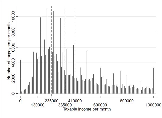
Figure 2: Contribution of different tax instruments: share of total tax revenue

Source: authors’ visualization based on data from OECD (2020).

Uganda increased its tax take in the 2010s, and the share of revenues from taxing individuals also
rose, from approximately 23 per cent in 2010 to over 25 per cent in 2016 (see Figures 1 and 2).
The contribution of PAYE alone was UGX2.4 trillion 7 of total tax revenue collected, constituting
about 16.6 per cent of total tax revenue in the 2017–18 fiscal year. For comparison, value added
taxes contributed similarly to gross revenues at 15.1 per cent; corporate and withholding taxes, the
other main contributors to direct taxes, constituted 6.9 per cent and 5.0 per cent respectively.
Overall, domestic tax (direct and indirect taxes) makes up 55.3 per cent of gross revenues, with
taxes on international trade contributing the rest (URA 2018; Waiswa et al. 2020).

The growth in PAYE revenue was enhanced by several reforms, including the adoption of an
electronic filing system for PAYE (e-tax system) that substantially simplified the filing procedure.
Before the roll-out of the e-tax system starting in September 2009, there was a highly manual tax
assessment and payment process in place. The e-tax system automated the registration, filing,
payment, and further processes with the aim of easing transactions so as to ultimately enhance
revenue collection, among other goals. The e-tax system was fully operating in all tax offices across
Uganda from February 2012 onwards.

In general, all employers have been required to obtain tax identification numbers (TINs) since the
introduction of the e-tax system (although this also pre-dated e-tax). According to Section 4(1) of
the Tax Procedures Code Act (Act 14 of 2014, of 1 July 2016), all employees are required to register
and acquire a TIN. However, in practice, employers are currently not required to report TINs for
all their employees, and employers cannot force their employees to acquire a TIN. Employers are

7
 In 2020, US$1 = UGX3,700.

 4

therefore not held to report all employees’ TINs by URA, to avoid them not reporting PAYE at
all for those employees.

Apart from income tax, any employed or self-employed Ugandan is subject to the local service tax
(LST), which is levied on wealth and income. Whether one is held to pay the LST, and the amount
of LST ultimately levied, depends on the type of (self-)employment and income earned (for an
overview and recent reforms to the LST, see Waiswa et al. 2020). For employees, the LST on
wages is also deducted by the employer, and the LST is a tax-deductible payment for employees.
The rates of the LST have been unchanged since 2008 (Local Government (Amendment) (No. 2)
Act 2008, of 7 July).

2.2 The income tax reform of 2012

With the fiscal year 2012–13, a major income tax reform came into effect. The government’s stated
motivation for the reform was to take into account inflationary effects. The tax schedule had been
the same for over ten years, and due to bracket creep an increasing number of low-income earners
such as teachers had become subject to tax. To counteract the significant revenue loss such reform
would obviously entail, the government decided to generate additional revenue by increasing taxes
on high incomes.

The reform consisted of two major changes. First, the whole tax schedule was shifted to the right.
That is, the threshold of the tax-free lowest band increased from UGX130,000 (or US$57) per
month to UGX235,000 per month, thus pushing it up by nearly 80 per cent. The third tax bracket,
ranging initially from UGX235,00 to UGX410,000, was split into two tax brackets taxed at ten per
cent and 20 per cent respectively. Second, the reform introduced an additional top tax bracket with
a marginal tax rate of 40 per cent for incomes exceeding UGX10,000,000 per month. Until then
the top marginal tax rate had been 30 per cent. 8
Table 1: Individual income taxation in Uganda since fiscal year 1997–98

 Monthly taxable income Tax rate
Pre-reform: Not exceeding 130,000 0%
1997–98 to Over 130,000, but not exceeding 235,000 10% of the amount exceeding 130,000
2011–12
 Over 235,000, but not exceeding 410,000 10,500 plus 20% of the amount exceeding
 235,000
 Over 410,000 45,500 plus 30% of the amount exceeding
 410,000
Post-reform: Not exceeding 235,000 0%
2012–13 and Over 235,000, but not exceeding 335,000 10% of the amount exceeding 235,000
onwards
 Over 335,000, but not exceeding 410,000 10,000 plus 20% of the amount exceeding
 335,000
 Over 410,000, but not exceeding 10,000,000 25,000 plus 30% of the amount exceeding
 410,000
 Over 10,000,000 2,902,000 plus 40% of the amount exceeding
 10,000,000

Note: all monetary values are in UGX.
Source: author’s compilation based on the Income Tax Act (of 1 July 1997, Cap 340 of the Laws of Uganda
2000) and the Income Tax (Amendment) Act 2012 (of 1 July).

8
 Tax rules are defined in the Income Tax Act (of 1 July 1997, Cap 340 of the Laws of Uganda 2000) and the Income
Tax (Amendment) Act 2012 (of 1 July).

 5

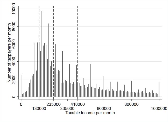
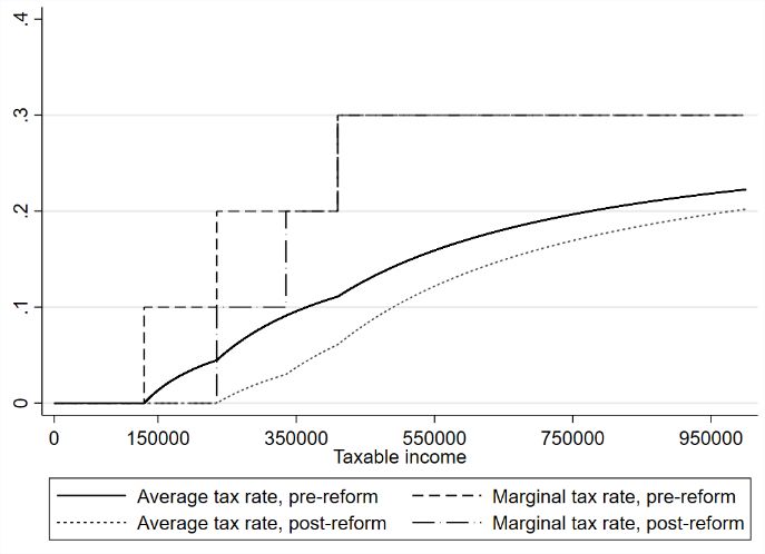
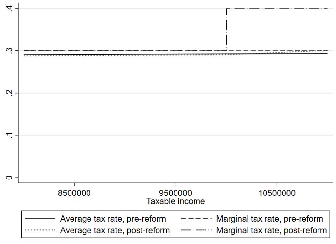
Figure 3: Marginal and average tax rates of individual income tax by monthly taxable income

Note: the upper panel shows tax rates from UGX0 to UGX11 million of taxable income. The lower two panels
concentrate on the tax rates at the bottom and the top, where the most pronounced changes in tax rates took
place. The lower left panel shows tax rates for taxable incomes less than UGX1 million, and the lower right panel
shows tax rates for taxable incomes more than UGX8 million. ‘Pre-reform’ refers to fiscal years before the 2012–
13 fiscal year. ‘Post-reform’ refers to the fiscal year 2012–13 and onwards. All monetary values are in UGX.
Source: authors’ schematic representation based on the Income Tax Act (of 1 July 1997, Cap 340 of the Laws of
Uganda 2000) and the Income Tax (Amendment) Act 2012 (of 1 July).

Table 1 and Figure 3 illustrate the PAYE rates applicable to resident individuals before and after
the reform. In terms of changes to average and marginal tax rates, the reform reduced marginal
and average tax rates for low- to middle-income taxpayers, and it increased the marginal and
average tax rates for those in the newly introduced top tax band. The reform did not affect marginal
taxes for incomes sitting in the tax bracket just below the newly introduced top tax bracket. The

 6

reform only marginally increased average tax rates for those sitting at the top of the second highest
tax bracket compared with those sitting in the top tax bracket in the reformed scheme.

Below we refer to the following five groups of taxpayers, based on how the reform affected their
marginal and average tax rates:

 1. ‘To zero’ taxpayers are the group of taxpayers with monthly taxable income in the range
 of UGX0 to UGX235,000. Those in the group with monthly taxable incomes between
 UGX130,000 to UGX235,000 experienced a reduction of tax rates to zero due to the
 reform.
 2. ‘MTR down’ taxpayers are the group of taxpayers with monthly taxable income in the
 range of UGX235,001 to UGX335,000, whose marginal tax rate went from 20 per cent to
 ten per cent, while average tax rates also fell.
 3. ‘ATR down, lower income’ taxpayers are the group of taxpayers with monthly taxable
 income in the range of UGX335,001 to UGX410,000, whose average tax rate fell while
 the marginal tax rate remained stable at 20 per cent.
 4. ‘ATR down, higher income’ taxpayers are the group of taxpayers with monthly taxable
 income in the range of UGX410,001 to UGX10,000,000, whose average tax rate fell while
 the marginal tax rate remained at 30 per cent. As taxable income approaches
 UGX10,000,000, the difference in average tax rates between pre- and post-reform
 becomes marginal.
 5. ‘Top taxpayers’ are the group of taxpayers with monthly taxable income in the range of
 UGX10,000,001 or higher.

3 Data and descriptive evidence

We use the universe of PAYE data extracted from URA databases. The monthly payroll tax data
includes information submitted by the employer through the e-filing system, such as basic salary,
allowable deductions, taxable income, and payable tax for each employee. It also includes
indicators of whether the taxpayer is subject to the resident tax schedule, and whether taxable
income is subject to the flat-rate tax for income from a second job. The data ranges from fiscal
year 2010–11 to fiscal year 2014–15 and is available on a monthly basis. Earlier data is not of
sufficient quality and coverage due to the roll-out of the e-tax system. For some employees falling
into the lowest tax-free tax band, data is available if the employer shared the information with
URA. Employees’ TINs are largely not known for the reasons provided above, and we thus cannot
create a panel of taxpayers.

Linking employers’ TINs across time is nevertheless possible, as employers’ TINs are recorded in
the data. This employer-based panel serves as an important robustness check: the data in digital
format does not cover all regions in the first years, because of the staggered implementation of the
e-tax system. Including tax region fixed effects or restricting the analysis to the same employers
allows us to control for the e-tax roll-out.

Non-resident taxpayers represent a negligible share of observations at fewer than 0.2 per cent, and
we therefore drop them from our analysis. We also exclude records of employees taxed at the flat
rate of 30 per cent for their second job subject to PAYE. They represent only around two per cent
of observations and are not our main interest of analysis.

 7

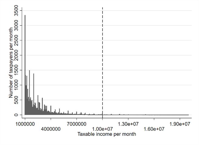
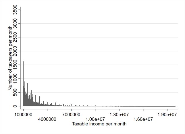
Table 2: Summary statistics of employees subject to PAYE

 2010–11 2011–12 2012–13 2013–14 2014–15
Taxable income Mean 1,027,101 1,031,467 1,169,879 1,169,773 1,088,942
 Median 354,750 350,000 400,000 400,000 440,000
 St dev. 14,339,589 5,512,124 4,135,703 4,362,415 4,576,946
Basic salary Mean 901,016 910,407 1,048,436 1,051,102 981,635
 Median 300,000 300,000 350,000 359,700 408,135
 St dev. 12,884,193 5,057,097 3,650,625 3,520,560 4,032,016
Payable tax Mean 246,028 247,136 287,143 285,476 256,371
 Median 34,455 33,500 23,000 23,000 34,000
 St dev. 4,301,466 1,651,306 1,556,276 1,653,639 1,754,052
Total payable taxes (in 528.44 731.30 1,024.77 1,193.45 1,379.61
billions)
Number of taxpayers Total 2,147,903 2,959,084 3,568,851 4,180,571 5,381,323

Note: all monetary values are in UGX and refer to monthly incomes. Non-resident employees and records of
employees taxed at the flat rate of 30 per cent for a second job subject to PAYE excluded.
Source: authors’ calculations based on URA PAYE administrative tax records.

Figure 4: Distribution of taxpayers by taxable income pre-reform and post-reform
 Taxable income up to UGX1 million Taxable income of UGX1 million or higher
 Pre-reform (2011–12)
 Post-reform (2013–14)

Note: in the pre-reform panels, dashed lines are the thresholds in the pre-reform tax schedule: (1) 130,000, (2)
235,000, (3) 410,000. In the post-reform panels, dashed lines are the thresholds in the post-reform tax schedule:
(1) 235,000, (2) 335,000, (3) 410,000, (4) 10,000,000. The size of a bin in the graph is UGX10,000. Incomes
exceeding UGX20 million are excluded from the figure.
Source: authors’ calculations based on URA PAYE administrative tax records.

 8

The overall number of employees subject to PAYE more than doubled between 2010–11 and
2014–15 (see Table 2). The median of basic salaries and taxable income (i.e. a basic salary plus any
applicable allowances, bonuses, etc.) steadily increased, although it moved sideways in 2013–14.
The mean of taxable income and basic salary also increased year on year, except for the last year
analysed. Payable tax accordingly shows a similar pattern across time. While the mean taxable
income goes down in 2014–15, total payable taxes from PAYE records increase alongside the
increasing number of taxpayers.

The distribution of taxable income changed between the pre-reform and post-reform fiscal years
(Figure 4), with less heaping to the left of the distribution. The graphs reveal a clear pattern of
round number bunching, with incomes clustering around multiples of 100,000 and similar round
values. Visually, no obvious bunching around the tax thresholds is identifiable.

Before and after the reform, the largest share of taxpayers falls consistently into the ‘ATR down,
higher incomes’ group, with around half of all observations (upper panel of Table 3). This share
further increases with the onset of the reform, from 44 per cent to 48 per cent. The second largest
group of taxpayers are those in the ‘to zero’ group, who pay no tax (or before the reform, little
tax). This share—consistent with the reform’s stated intention to alleviate the tax burden at the
lower end of the wage distribution—decreased from 37 per cent pre-reform to 29 per cent. The
share of ‘top taxpayers’ did not change to a large extent.

The lower panel of Table 3 shows for each taxpayer group how the average taxable income of that
group relates to the average taxable income of the universe of PAYE taxpayers. Around the
reform, the average taxable income of the ‘ATR down, higher incomes’ taxpayers group goes from
151 per cent times the average taxable income to 139 per cent, thus clearly declining by 8.6 per
cent. For top taxpayers we find an even more sizable decline of nearly 20 per cent in declared
average taxable income, from 2,357 per cent to 1,977 per cent. The latter group thus on average
has a taxable income roughly 20 times that of the average taxable income.
Table 3: Shares of taxpayers and mean taxable income by taxpayer group

 Fiscal year ‘To zero’ ‘MTR down’ ‘ATR down, ‘ATR down, ‘Top
 taxpayers taxpayers lower income’ higher income’ taxpayers’
 taxpayers taxpayers
Share of 2010–11 37% 11% 6% 45% 0.9%
taxpayers 2011–12 37% 12% 6% 44% 1.0%
 2012–13 29% 15% 7% 48% 1.2%
 2013–14 28% 16% 7% 48% 1.2%
 2014–15 23% 15% 10% 51% 1.2%
Mean taxable 2010–11 14% 27% 36% 152% 2428%
income 2011–12 14% 27% 36% 151% 2357%
(as a share of
 2012–13 13% 24% 32% 139% 1977%
average income)
 2013–14 13% 24% 32% 139% 1913%
 2014–15 14% 26% 35% 131% 1924%

Note: monthly taxable income for ‘to zero’ taxpayers: UGX0–235,000; ‘MTR down’ taxpayers: UGX235,001–
335,000; ‘ATR down, lower income’ taxpayers: UGX335,001–410,000; ‘ATR down, higher income’ taxpayers:
UGX410,001–10,000,000; ‘top taxpayers’: UGX10,000,001 or higher. Grey-shaded cells are for post-reform time
points.
Source: authors’ calculations based on URA PAYE administrative tax records.

In the following we concentrate on the ‘top taxpayers’ and the highest earning employees in the
‘ATR down, higher incomes’ taxpayer group, situated just below the top group in the taxable
income distribution. Specifically, we compare the ‘top taxpayer’ group, who constitute roughly one

 9

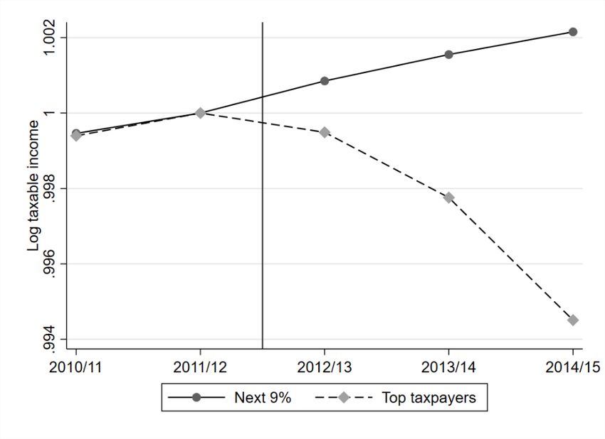
per cent, with the next nine per cent of taxpayers, ranging from the 90th percentile to the threshold
of the ‘top taxpayers’ (roughly to the 99th percentile). We opt to use a smaller set of the ‘ATR
down, higher incomes’ taxpayer group as the group is very large and thus likely heterogeneous, as
observations are located further away from the threshold of the top taxpayer group. Furthermore,
the difference in the average tax rates pre- and post-reform becomes negligible, making the change
in the marginal tax rate the only difference between the two groups. We thus refer to the ‘top
taxpayer’ group as the treatment group, and the next nine per cent in the distribution as the control
group, in the descriptive and econometric analysis below, unless indicated otherwise.
Table 4: Mean monthly incomes (in millions) for the ‘top taxpayers’ treatment and control groups

Fiscal year Treatment group (‘top taxpayers’) Control group (‘next 9%’)
2010–11 24.937 3.901
2011–12 24.309 3.949
2012–13 23.128 3.993
2013–14 22.386 4.035
2014–15 20.946 4.075
Pre-reform 24.623 3.925
Post-reform 22.153 4.034
Note: treatment group (‘top taxpayers’): monthly taxable income UGX10,000,001 or higher. Control group (‘next 9
per cent’ = p90 up to the ‘top taxpayers’ group threshold): monthly taxable income UGX2,117,900–10,000,000.
‘Pre-reform’ refers to the mean monthly taxable income for fiscal years 2010–11 and 2011–12. ‘Post-reform’
refers to the following three fiscal years. Grey-shaded cells are for post-reform time points. All monetary values
are in UGX.
Source: authors’ calculations based on URA PAYE administrative tax records.

Figure 5: Parallel trends for treatment group (‘top taxpayers’) and control group (‘next 9 per cent’)

Note: incomes are normalized to one for both groups in 2011–12. The vertical line indicates the reform time in
July 2012.
Source: authors’ calculations based on URA PAYE administrative tax records.

 10

Table 4 shows the mean monthly taxable income for the treatment and control groups. Between
fiscal years 2011–12 and 2014–15, mean monthly taxable income declines by 16 per cent for the
treatment group; it also declines consistently in a year-on-year perspective, and decreases by ten
per cent when we lump together all pre- and all post-reform observations. By contrast, mean
monthly taxable income increases consistently for the control group, increasing by 4.5 per cent
between fiscal years 2011–12 and 2014–15, and by 2.78 per cent when we compare pre- and post-
reform data.

Figure 5 plots the mean log taxable incomes for the treated ‘top taxpayers’ and the control group.
The parallel trends assumption appears to hold for the (admittedly short, two-year) period before
the reform. After the reform, the log income drops noticeably for treated individuals.

4 Methodology

We aim to examine whether, and if so by how much, taxpayers reacted to the increase in the top
marginal tax rate. It might be that high-income individuals put in less work, or that employees and
employers colluded to report lower incomes than they would have done in the absence of the
reform. Such responses are captured by the elasticity of taxable income, i.e. the percentage change
of taxable income with respect to a percentage change in the net-of-tax rate. The net-of-tax rate is
defined as one minus τ, where τ represents the marginal tax rate.

We employ difference-in-differences (DiD) analysis to estimate top taxpayers’ response in terms
of changes to their taxable income in response to the increase in the marginal tax rate they faced
due to the reform. Specifically, we consider the taxpayers subject to the tax increase (that is, people
with monthly taxable income exceeding UGX10,000,000) as the treated group, and those just
below that threshold as the control group (that is, the ‘next nine per cent’, situated between
UGX2,117,900 and UGX10,000,000 monthly taxable income). In other words, the control group
includes people from the 90th to the 99th percentiles. In the DiD analysis we then basically compare
the mean taxable income across these two otherwise similar groups before and after the reform.
As discussed in Section 2.2, individuals in the control group experienced no changes in the
marginal tax rate and only a minor reduction in the average tax rate.

We thus estimate the basic DiD regression equation:

 = β0 + β1 Treat + ∑ β2, Year + ∑ β3, Month + β4 (Treat After ) +
 β5 Tax office + ε [1]

where is the outcome variable log taxable income for observation i, tax office j, year t, and
month m, Treat is a dummy variable that takes value one when the individual belongs to the
treatment group, Year refers to dummies for each tax year, and Month refers to month
dummies. The variable of interest is the coefficient β4, which is our DiD estimate for the
interaction term (Treat After ), which takes value one when an observation is treated and
observed post-reform. As different parts of the country introduced the e-tax system at different
points in time, we also add fixed effects for tax office, Tax office , when estimating equation [1].

We add group-specific linear trends based on the pre-treatment period in some specifications, to
account for group-wise trend heterogeneity. For example, in this way we allow a different trend in
taxable incomes for the treatment group than for the control group. In addition, we examine
heterogeneous responses by splitting the treatment group into two: the top one to 0.5 per cent,

 11

and the top 0.5 per cent. As further robustness checks, we vary the lower cut-off point for the
control group and study response heterogeneity by size of employer and tax office.

We use the DiD estimate β4 to calculate the uncompensated elasticity of taxable income using the
following equation:
 
 = (1− ) [2]
 1− 

5 Results

5.1 Main results

Table 5 presents DiD estimation results using different specifications. The upper panel provides
the basic DiD results, whereas results in the lower panel have been adjusted for group-specific
pre-treatment trends. Models (2) and (4) are weighted using income weights to reflect relative
contribution to total revenues, as is commonly done in the literature on the elasticity of taxable
income.
Table 5: Benchmark DiD results for treatment group ‘top taxpayers’

 ‘Top taxpayers’ ‘Top taxpayers’, censored
 (1) (2) (3) (4)
 Simple Weighted Simple Weighted
Basic:
Treati*Aftert -0.0779** -0.317** -0.0765** -0.174***
 (0.0343) (0.129) (0.0342) (0.0611)
Year and month dummies Yes Yes Yes Yes
R-squared 0.561 0.627 0.562 0.705
Implied elasticity 0.5453** 2.219** 0.5355** 1.218***
 (0.2401) (0.903) (0.2394) (0.4277)
Pre-trend controls:
Treati*Aftert -0.0828** -0.322** -0.0823** -0.181***
 (0.0343) (0.129) (0.0342) (0.0611)
Year and month dummies Yes Yes Yes Yes
R-squared 0.553 0.621 0.551 0.698
Implied elasticity 0.5796** 2.254** 0.5824** 1.267***
 (0.2401) (0.903) (0.2394) (0.4277)
Observations 2,015,531 2,015,531 (censored 2,039)

Note: columns (2) and (4) present weighted least squares estimates with income used as weights. In columns (3)
and (4), incomes exceeding the top one per cent threshold among the treated group (that is, income above 0.01
per cent of all income earners) are censored to the threshold value. In the lower panel, we first predict income
growth for post-reform years from pre-reform data separately for the treatment and control groups; we then
subtract the trend from post-reform data, and use these values as outcomes. The estimated models include tax
office fixed effects. Standard errors clustered at the firm level in parentheses. *** p

to around two. Whether estimates are adjusted for possibly different pre-trends does not appear
to make a marked difference for the size of our estimates.

As large outliers at the top of the distribution might be driving the results, we further estimate the
same equation censoring the taxable incomes of the top of the treatment group (models 3 and 4).
Specifically, we censor taxable incomes at the 99.99th percentile for each year. 9 Capping taxable
incomes at the top makes a large difference: the income-weighted elasticity drops from 2.2 to 1.2.
This suggests that the very high elasticity found in the basic specification is driven by a few large
observations.

To further study this matter, we split the treatment group into two halves: a lower half with
employees with monthly taxable incomes between the 99th and 99.5th percentiles, and an upper half
with those in the top 0.5 per cent of the distribution, censored at the 99.99th percentile. Estimates
for both groups are presented in Table 6, and results are in line with our previous findings. The
response among the lower half of the ‘top taxpayers’ is more muted, with an elasticity of 0.28
(income-weighted results). By contrast, the explanation for the high elasticity found in the basic
regression above seems to stem from the response of the very top taxpayers. For the top half of
the treatment group, we find an elasticity of 1.26.
Table 6: DiD results for the upper and lower halves of the treatment group ‘top taxpayers’

 Top 1–0.5% Top 0.5%, censored
 (1) (2) (3) (4)
 Simple Weighted Simple Weighted
Basic:
Treati*Aftert -0.0405*** -0.0397*** -0.113*** -0.180***
 (0.0107) (0.0099) (0.0408) (0.0526)
Year and month dummies Yes Yes Yes Yes
R-squared 0.316 0.434 0.539 0.793
Implied elasticity 0.2835*** 0.2779*** 0.791*** 1.260***
 (0.0749) (0.0690) (0.2856) (0.3682)
Observations 1,913,501 1,913,497 (censored 2,039)

Note: columns (2) and (4) present weighted least squares estimates with income used as weights. In columns (3)
and (4), incomes exceeding the top one per cent threshold among the treated group (that is, income above 0.01
per cent of all income earners) are censored to the threshold value. The estimated models include tax office fixed
effects. Standard errors clustered at the firm level in parentheses. *** p

Table 7: Heterogeneity analysis for treatment group ‘top taxpayers’ in small and large firms, censored

 Baseline Small firms Large firms
 (1) (2) (3) (4) (5) (6)
 Simple Weighted Simple Weighted Simple Weighted
Basic:
Treati*Aftert -0.0765** -0.174*** -0.0397** -0.187*** -0.146* -0.225*
 (0.0342) (0.0611) (0.0199) (0.0619) (0.0813) (0.115)
Year and month dummies Yes Yes Yes Yes Yes Yes
R-squared 0.562 0.705 0.553 0.701 0.577 0.714
Implied elasticity 0.5355** 1.218*** 0.2779** 1.309*** 1.022* 1.575*
 (0.2394) (0.4277) (0.1393) (0.4333) (0.5691) (0.805)
Observations 2,015,531 989,784 1,025,747

Note: we use median numbers of employees by firm to define large and small firms. The estimated models
include tax office fixed effects. There are 2,039 censored observations. Standard errors clustered at the firm level
in parentheses. *** p

bracket. Since this phenomenon may not necessarily be due to the tax system, the high elasticities
reported may not be fully caused by the tax reform alone.
Table 8: Heterogeneity analysis for treatment group ‘top taxpayers’ in MTO, LTO, and all other tax offices,
censored

 LTO firms MTO firms All other tax offices
 (1) (2) (3) (4) (5) (6)
 Simple Weighted Simple Weighted Simple Weighted
Basic:
Treati*Aftert -0.0965* -0.199** -0.0247 -0.0485 -0.0416 -0.0929
 (0.0509) (0.0783) (0.0228) (0.0591) 0.0404 (0.0916)
Year and month dummies Yes Yes Yes Yes Yes Yes
R-squared 0.591 0.710 0.489 0.668 0.513 0.685
Implied elasticity 0.6755* 1.393** 0.1729 0.3395 0.2912 0.6503
 (0.3563) (0.5481) (0.1596) (0.4137) (0.2828) (0.6412)
Observations 1,240,972 337,085 437,474

Note: columns (1) and (2) show estimates for firms that fall under the LTO. Columns (3) and (4) present
estimates for firms that fall under the MTO. Columns (5) and (6) includes all other tax offices; we further include
tax office fixed effects in these specifications. There are 2,039 censored observations. Standard errors clustered
at the firm level in parentheses. *** p

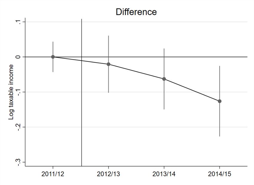
The size of the estimate thus seems to hinge significantly on the composition of the treatment
group, rather than on the exact definition of the control group.

We further study how taxable incomes react across time through the lens of event study methods.
Specifically, in our econometric specification we replace the interaction term between the
treatment indicator and after-dummy (the DiD estimate) with interactions of the treatment group
indicator with dummies for all years. Estimation results (with corresponding confidence intervals)
are plotted in Figure 6. The graph indicates that before the reform (2011–12), there is no difference
between treatment and control, as should be the case. After the reform, a difference starts to
emerge, and the response seems to unfold gradually, with the latest year showing the largest drop
in treatment group incomes. This may be an indication that taxpayers cannot adjust their earnings
immediately but do so slowly over time.
Figure 6: Event study plots for the treatment group ‘top taxpayers’, censored

Note: difference estimated using the DiD regression model. The vertical line indicates the time of the reform in
July 2012.
Source: authors’ calculations based on URA PAYE administrative tax records.

5.3 Investigating possible mechanisms

To understand better the potential mechanisms underlying the response of the ‘top taxpayers’
group to the marginal tax rate increase, we investigate more closely the 100 firms whose PAYE
records drop the most after the reform. For that purpose, we first identify these firms in the PAYE
balanced panel data, and then we merge information from these firms with the corporate income
tax (CIT) returns. 12 Second, in order to create a comparison group, we check the size of the firms
that experience the largest drop in PAYE income paid to their employees based on their sales, and
we identify other firms subject to CIT that show similar sales figures to the firms with the largest
PAYE income drops. This leaves us with around 3,500 firms for the comparison group. Finally,

12
 In URA’s e-tax system, a company (i.e. corporate or unincorporate income taxpayer, or a unit trust, and any entity
other than a partnership firm deriving income from business or profession) files an income tax return form for a non-
individual. The return data generated from this form is referred to as CIT returns data in this paper.

 16

we identify the firms from the comparison group in the PAYE balanced panel records, and we
further restrict the comparison group to firms that have employees in the highest tax bracket. This
exercise leaves us altogether with 321 firms with matched PAYE balanced panel and CIT records
that fulfil the criteria set out above.

Table 10 presents average log sales, costs, profits, proposed dividends, 13 and PAYE income, and
their differences between before and after the tax reform, for firms with the largest drop in PAYE
incomes and our choice of comparable firms. We find that firms with the largest drop in PAYE
incomes decrease their sales and costs after the reform, but log profits and proposed dividends
increase. By contrast, among firms in the comparison group, proposed dividends decrease,
although their sales, costs, and profits are larger after the reform. This points to lower economic
activity for the firms with the largest drop in PAYE incomes compared with otherwise similar
firms. Nevertheless, these firms at the same time propose larger dividends to be paid out to
shareholders (see DiD values in Table 10). Following our definition of firms with the largest drop
in PAYE incomes, their PAYE incomes decrease after the reform. The comparison group’s PAYE
incomes increase, which makes the difference between two groups substantial. To put it simply,
firms whose employees’ taxable incomes (i.e. PAYE incomes) fall report an increase in profits and
dividends. Firms with no such change in PAYE incomes see higher economic activity after the
reform, but they do not increase dividends.

The above analysis cannot be interpreted as causal evidence; we are discussing strictly descriptive
evidence. It nevertheless clearly points to one possible mechanism, namely income shifting
between PAYE incomes and dividends.
Table 10: Descriptive evidence of average sales, costs, profits, proposed dividends, and salaries for largest-drop
and other firms

 Log sales Log costs Log profits Log Log PAYE No. of firms
 proposed income
 dividends
Largest-drop firms Before 22.97 22.43 20.15 22.45 2.65 100
 After 22.67 22.27 20.29 22.51 2.30 100
 Difference -0.30 -0.16 0.14 0.06 -0.35
Other firms Before 23.07 22.59 20.61 20.94 5.23 321
 After 23.43 22.84 20.85 20.84 6.12 321
 Difference 0.36 0.25 0.24 -0.10 0.89
 DiD -0.66 -0.41 -0.11 0.16 -1.24

Note: largest-drop firms are firms that have the largest drop in PAYE incomes (= log PAYE income) from the ‘top
taxpayers’ group after the reform. Other firms are firms that have similar log sales to largest drop firms and have
employees in the ‘top taxpayers’ group in the PAYE balanced panel data. Log sales, log costs, log profits, and log
proposed dividends are calculated from CIT returns data, and log PAYE incomes from PAYE balanced panel
records.
Source: authors’ calculations based on URA PAYE and CIT administrative tax records.

13
 In the Ugandan context, proposed dividends refer to expected provisional dividends declared by the firm at the
beginning of its income year on the CIT tax form. If the firm pays the dividends proposed in its provisional returns
at the end of the fiscal year, the proposed dividends are considered final; otherwise the dividends are amended in the
final return.

 17

5.4 Results for other tax brackets

Finally, we turn to discuss results for the other taxpayer groups who experience a decline in tax
rates (see detailed results in the Appendix). These include those in the two groups at the bottom
of the income distribution, whose marginal tax rate declines by ten percentage points (‘to zero’
taxpayers and ‘MTR down’ taxpayers in Table 3), and the group whose average tax rate drops
significantly (‘ATR down, lower incomes’). The taxable income developments for these groups are
compared with those in a control group that consists of individuals earning UGX410,000– 704,447
(the 70th percentile) a month. Results in Table A2 in the Appendix indicate that incomes increase
more for these groups than among the controls, but the treatment impacts are small, and their
significance is sensitive to whether or not possibly different linear trends are controlled for. The
corresponding elasticities are also small, at around 0.1. 14 In terms of estimating the reform’s
dynamic impacts on revenue, the reactions of the ‘top taxpayers’ group seem to dominate.

6 Revenue implications

Based on the above findings on the elasticity of taxable income, we now turn to the question of
how revenue is affected. In particular, we are interested in how far the behavioural response along
the taxable income margin generates less revenue. For that purpose, we first calculate the actual
tax revenues recorded by URA for all fiscal years. Second, we compare those values to simulated
revenue in the absence of behavioural responses to the reform. For the latter we apply the post-
reform tax schedule to the uprated pre-reform taxable incomes. The uprating factor for incomes
is a difference in the mean income growth between the control and treatment groups. 15 Finally,
comparing the actual revenue with the simulated revenue reveals how much revenue the
behavioural responses cost.

We first perform this exercise for the ‘top taxpayers’ group before turning to the other groups. We
finally close this section with the overall implications for PAYE revenues.

6.1 Revenue implications for the top group

We first calculate actual revenues gathered from the control and treatment groups, as defined for
the analysis of top taxpayers in Section 5, for the different fiscal years. Columns 1 and 2 of Table
11 show that the actual revenues from PAYE increase over the time span analysed for both groups,
but more so for the treated group, which faces an increase in the marginal tax rate.

For the counterfactual scenario of the ‘top taxpayers’ treatment group, uprated incomes are seven
per cent higher than actual incomes in the post-reform period. This uprating factor of seven per
cent reflects a conservative mean estimate for the DiD results discussed in Section 5; this would
correspond, for example, to the simple estimates in columns (1) and (3) in the lower part of Table
5, or to weighted estimates in the case of the firm panel in Table 9, column (4). To sum up,
simulated revenues are obtained by first uprating employees’ taxable incomes in the treatment

14For the group whose marginal tax rate does not change, an intensive margin elasticity cannot be calculated (division
by zero). Individuals in this group also report higher incomes after the reform. If there were significant income effects,
they would instead lower their earnings since their average tax rate declined. This channel is probably not so important
for salaried workers with mid-level incomes in a poor country. Instead, it is more likely that the positive response
arises from (a discrete decision about) starting to report incomes when the tax rate falls.
15
 We do not use estimates of the DiD regressions from Section 5 as the uprating factor, because estimates depend
significantly on the chosen specifications. Instead, we use a simple illustrative calculation of mean income growth.

 18

group by seven per cent for the post-reform period; second, we use the post-reform tax rules to
calculate the hypothetical payable taxes by employee; then we sum every employee’s taxes together
for each year, which is finally our hypothetical revenue. This simulated revenue represents how
much revenue would be collected if there were no behavioural responses to the reform.

The results suggest that the mean annual revenue loss due to behavioural reactions amounts to
approximately UGX46 billion (Table 11, columns (2) and (3), mean post-reform UGX435 minus
UGX389 billion), or 12 per cent of the treated group actual revenues. The reason why the relative
revenue loss (12 per cent) is greater than the percentage change in taxable income (seven per cent)
is because the average tax rate increases when incomes are increased.

Needless to say, this calculation is a simplified exercise, as we only take into account the PAYE
part of the income tax, and we disregard any revenue changes stemming from taxes on small
business owners. On the other hand, if some part of the behavioural response stems from income
shifting between different tax bases rather than from a real behavioural reduction, our revenue
loss calculations are upwardly biased. This is likely the case here, since those at the very top of the
income distribution appear to react to the reform more. If these individuals include corporation
owners, they might react to the reform by lowering the salaries their corporations pay to
themselves and using other forms of compensation (such as dividend income) instead (see also
the discussion in Section 5.3). To the extent that these other payouts are within the tax net, the
overall revenue consequences would be smaller.
Table 11: PAYE actual revenues and counterfactual simulated revenues in the case of no behavioural changes
for ‘top taxpayers’ and the control group

Fiscal year Actual revenue, control Actual revenue, treatment Simulated revenue,
 group group ‘top taxpayers’ treatment group ‘top
 taxpayers’
 (1) (2) (3)
2010–11 182 119
2011–12 346 202
2012–13 428 341 378
2013–14 500 389 433
2014–15 549 439 495
Mean, pre-reform 264 161
Mean, post-reform 493 389 435

Note: all monetary values are in UGX billions. Column (1) reports the actual revenues from the control group (the
next nine per cent), while column (2) does the same for the treatment group ‘top taxpayers’. ‘Simulated revenue,
treatment group’ reflects revenues generated by the treatment group for the post-reform years if there are no
behavioural responses to the reform. Grey-shaded cells are for post-reform time points.
Source: authors’ calculations based on URA PAYE administrative tax records.

The above back-of-the envelope calculation raises the question of what the revenue-maximizing
top tax rate would be in the Ugandan context. Theory has shown (e.g., Piketty and Saez 2013) that
the revenue-maximizing top tax rate in a non-linear income tax system is:
 1
 ∗ = 1+ ∗ [3]

where is the Pareto parameter estimated from fitting a Pareto distribution using income data,
and e is the elasticity of taxable income. We have estimated the Pareto parameter on the basis of
the Ugandan PAYE data for incomes exceeding the threshold value of the highest marginal tax
bracket. The estimates are in the range of 1.7 to 1.9 for the different years. These estimates suggest
that the Ugandan earnings distribution is quite uneven. Since the Pareto parameter measures the

 19

thinness of the upper tail, the results indicate that the Ugandan earnings data has a fairly fat upper
tail. Other things being equal, this raises the revenue-maximizing top tax rate.

With an elasticity equal to, say, 0.5, the revenue-maximizing top tax rate would then amount to
around 53 per cent. We should note that this tax rate also includes the tax burden stemming from
indirect taxes. When we take indirect taxes into account, the current Ugandan top tax rate is
approximately 50 per cent. 16 This would suggest that the current Ugandan top tax rate is quite
close to the theoretical rate maximizing revenues from top earners. It is worth bearing in mind
that the above calculation disregards various considerations, including possible income shifting
and the impacts of taxes on the extensive margin (the share of formal sector employment in the
economy).

6.2 Revenue implications for other tax brackets

Similarly as for the top taxpayers, we calculate the actual and simulated tax revenues for the other
treatment groups and the respective control group in Table 12. The actual and simulated revenues
for the other treatment groups (‘to zero’, ‘MTR down’, and ‘ATR down, lower incomes’) are shown
in columns (1–5), and actual revenue from the control group (monthly incomes UGX410,000–
704,447, the threshold of the 70th percentile) pertaining to these treatment groups is shown in
column (6).
Table 12: PAYE actual revenues and counterfactual simulated revenues in the case of no behavioural changes
for other treatment groups

Fiscal year ‘To zero’ ‘MTR down’ ‘ATR down, lower incomes’ Control group
 (1) (2) (3) (4) (5) (6)
 Actual Actual Simulated Actual Simulated Actual
 revenue revenue revenue revenue revenue revenue
2010–11 4.3 4.1 4.6 22.9
2011–12 5.2 6.9 7.0 35.8
2012–13 0 2.7 2.0 4.5 3.8 36.0
2013–14 0 3.3 2.6 5.5 4.7 50.0
2014–15 0 4.1 3.2 10.7 9.3 71.7
Mean, pre-reform 4.8 5.5 5.8 29.4
Mean, post-reform 0 3.4 2.6 6.9 5.9 52.6
Note: all monetary values are in UGX billions. Columns (1–5) show revenues, both actual and simulated, for
treatment groups. Column (1) presents the actual revenue for the treatment group ‘to zero’ (incomes
UGX130,000–235,000). Column (2) does the same for the treatment group ‘MTR down’ (incomes UGX235,001–
335,000). The numbers in column (3) are simulated revenues that would be available from the treatment group
‘MTR down’ after the reform if there were no behavioural responses to the reform. Column (4) shows the actual
revenue for the treatment group ‘ATR down’ (incomes UGX335,001–410,000); simulated revenues without
behavioural responses for the same treatment group are in column (5). Column (6) reports the revenues from the
control group, which has incomes UGX410,000–704,447 (the 70th percentile). Grey-shaded cells are for post-
reform time points.
Source: authors’ calculations based on URA PAYE administrative tax records.

The revenue calculations in Table 12 follow the changes in tax rates for the treatment groups. As
anticipated, the actual revenues of all treatment groups decrease when marginal and average tax
rates fall after the income tax reform of 2012. However, actual revenues increase steadily every

16 1− 
 Calculated as 1 − , where = 0.4 refers to the top marginal income tax rate and = 0.2 to the approximate
 1+ 
effective consumption tax rate, which includes value-added tax and excises.

 20