The effects of the coronavirus pandemic in emerging markets and developing economies: An optimistic preliminary account - Brookings Institution

BPEA Conference Drafts, June 25, 2020

The effects of the coronavirus pandemic in
emerging markets and developing economies: An
optimistic preliminary account

Pinelopi Koujianou Goldberg, Yale University, CEPR, and NBER
Tristan Reed, World Bank Development Research Group

Conflict of Interest Disclosure: The authors did not receive financial support from any firm or person for this
paper or from any firm or person with a financial or political interest in this paper. Pinelopi Goldberg was Chief
Economist of the World Bank Group until March 2020, received compensation from the World Bank in that
capacity, and is currently a non-resident Senior Fellow at the Peterson Institute for International
Economics. Tristan Reed is an economist for the World Bank. They are currently not officers, directors, or
board members of any organization with an interest in this paper. No outside party had the right to review this
paper before circulation. The views expressed in this paper are those of the authors and do not necessarily
reflect those of the World Bank or Yale University.

The Effects of the Coronavirus Pandemic in Emerging Market and Developing Economies:
 An Optimistic Preliminary Account∗

 Pinelopi Koujianou Goldberg1 and Tristan Reed2

 1
 Yale University, CEPR, and NBER
 2
 World Bank Development Research Group

 Prepared for Brookings Papers on Economic Activity Conference on June 25, 2020

 June 22, 2020

 Abstract

 Early in 2020, the general expectation was that the coronavirus pandemic’s effects would
 be more severe in developing countries than in advanced economies, both on the public
 health and economic fronts. Preliminary evidence as of June 2020 supports a more
 optimistic assessment. To date, most low- and middle-income countries have a
 significantly lower death toll per capita than richer countries, a pattern that we attribute
 primarily to a younger population and limited obesity. On the economic front, emerging
 market and developing economies (EMDEs) have seen massive capital outflows and large
 price declines for certain commodities, especially oil and non-precious metals, but these
 changes are in line with earlier commodity price shocks. While there is considerable
 heterogeneity in how specific countries will be affected in the short and medium run, the
 overall picture in EMDEs seems to be typical of a commodity price bust and will likely
 play out through familiar channels. If the disease burden is ultimately not as dire in these
 countries, this observation leaves us cautiously optimistic that the largest EMDEs,
 especially those not reliant on energy and metal exports, could recover quickly. In the
 long run, the highest costs may be due to the indirect effects of virus containment policies
 on poverty, health and education as well as the effects of accelerating deglobalization on
 EMDEs. An important caveat is that there is still considerable uncertainty about the future
 course of the pandemic and the consequences of new waves of infections.

 JEL Classification: I15, I18, O10, O57
 Keywords: Coronavirus, Pandemic, Emerging Markets, Developing Countries

 -----------------------------------------------------------------------------------------------------------
 ∗ E-mail: penny.goldberg@yale.edu, treed@worldbank.org. We thank our discussants, Sebnem Kalemli-
 Ozcan and Michael Kremer, as well as the editor, Janice Eberly, for many useful comments on an earlier
 draft. We are also grateful to DFID, UK for sharing with us their weekly “C19 Economic Evidence
 Roundups” with up-to-date information on the impact of the crisis in several developing countries. All data
 in this article are as of June 20, 2020.

Introduction

 As the COVID-19 health crisis spread throughout the world to reach low- and middle-income
countries in South Asia, Sub-Saharan Africa, and Latin America, the international community
became increasingly anxious about potentially catastrophic effects of the crisis there. In the early
months of 2020, the consensus was that such countries would be hit much harder than advanced
economies both on the public health and economic fronts. The Managing Director of the IMF,
Kristalina Georgieva, noted in an IMF podcast on April 9: “Just as the health crisis hits
vulnerable people hardest, the economic crisis hits vulnerable countries hardest.” The President
of the World Bank Group, David Malpass, estimated that the COVID crisis would push 60
million people in developing countries into extreme poverty. And in a recent poll of IGM’s
Economic Experts Panel, the majority of polled economists (including one of the coauthors of
this study) agreed that the “economic damage from the virus and lockdowns will ultimately fall
disproportionately hard on low- and middle-income countries.” Against this backdrop, the
message of this paper is cautiously optimistic: we find that to date, developing countries have
fared relatively well in terms of public health outcomes. And even on the economic front, while it
is premature to make any predictions regarding the medium- and long-term economic effects of
the crisis, there are encouraging signs regarding the short-term economic recovery of several
countries. We caveat our optimism by acknowledging that the health crisis has not yet played out,
and there is still considerable uncertainty about the future course of the pandemic and the
likelihood of future infection waves. Our optimism regarding the short run is counterbalanced by
our concern regarding the long run impact of the crisis arising from the indirect effects of
containment policies, especially the disruption of health and education services and increase in
extreme poverty, as well as from the acceleration of the deglobalization trend with its trade and
immigration policy implications.
 The paper provides preliminary evidence on the public health and short-run economic effects
of the COVID-19 crisis in developing countries along with some speculation about the long run.
The term “developing countries” will be used throughout the paper to include all “emerging
market and developing economies” – EMDEs henceforth. We start with an important qualifier:
EMDEs include an enormously diverse set of societies and economies. In the context of the
COVID-19 crisis in particular, it is useful to keep in mind that the set contains countries such as
Vietnam, which as of Jun 20, 2020 reports zero deaths due to COVID-19 and has generally been
 2

minimally affected by the crisis; Brazil, which as of June 20 reports 50,050 deaths; and
Zimbabwe, which has just five ICU beds, yet as of June 20, reports only 4 deaths due to COVID-
19. Nevertheless, what these countries have in common, both from a public health and an
economic standpoint, seems in the context of the current crisis more important than how they
differ. On the public health front, a distinct characteristic of many EMDEs is the low capacity of
the health care sector as proxied by number of hospital beds, medical equipment, and medical
personnel. On the economic front, the very term “developing” countries signifies vulnerabilities
that make these countries potentially more susceptible to economic contraction following a health
crisis. Further, while adverse economic effects in advanced economies are due to these countries’
(justified) efforts to contain the virus, adverse economic effects in EMDEs are to be expected due
to spillovers from advanced economies’ policies, independent of EMDE’s own policies. EMDE’s
own health and economic policies can amplify or reduce these spillover effects; but they cannot
avoid them.
 Our analysis is structured in two parts corresponding to the public health and economic
effects respectively. We start by examining how well countries have fared in the current crisis
from a public health perspective. Our measure of COVID-19 outcomes is “deaths per million”.
We chose this measure both because it is widely available, and because – measurement
challenges notwithstanding – it is less susceptible to concerns regarding biases that plague
statistics on positive case counts or hospitalizations. We document a robust positive association
between per-capita income and “deaths per million”: the higher the per capita income, the higher
the number of deaths per million. Hence, the global cross-country comparison exhibits the exact
opposite pattern from what has been widely documented within countries at specific locations: at
the global level, COVID-19 seems to be primarily a rich country problem; within municipalities,
however, it is the socioeconomically disadvantaged groups who suffer the most. 1 The spatial
pattern of coronavirus mortality is interesting as it may provide insight both into the political
economy of policy responses (and resistance to them) and into appropriate policies going
forward. Our analysis demonstrates that a large part of this positive correlation between
countries’ per-capita income and deaths per million can be explained through demographics (age)
and obesity. Whatever the source of this pattern, it gives a ray of hope to governments with fewer
1
 Interestingly, the spatial pattern of COVID mortality within countries exhibits the same pattern. For example, in
Italy, it was Lombardy, one of the wealthiest regions of the country, that had the highest death toll. Similarly, in the
United States, New York State, New York City in particular, had the highest deaths per capita in the country; but
within New York City, it was the socioeconomically disadvantaged who were affected the most.
 3

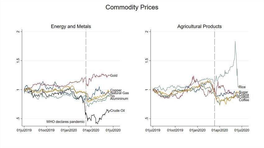
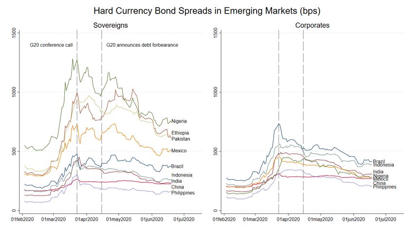
resources: it suggests that tragic as the loss of life may have been, it was not as large as
anticipated. This is positive, both because lives were spared and because it means that – to the
extent that this pattern does not change in the future – countries may be able to ease containment
measures and focus on the economic fallout that has been significant.
 Next, we examine the short-run economic effects. We focus on financial data, since financial
markets reacted immediately to the COVID news, and available data reflect this reaction – in
contrast, data on macroeconomic variables become available with a delay and currently exist for
only a handful of countries. Early March saw unprecedented portfolio outflows from EMDEs
accompanied by sharp depreciations of several currencies, an increase in bond spreads, a collapse
of commodity prices and with them of revenues from commodity exports. These developments
raised serious concerns about the solvency and general economic prospects of several EMDEs.
However, data from subsequent months present a more optimistic picture. Based on estimates of
broader measures of capital we show that while capital outflows have been severe, they are likely
within the range observed during earlier commodity price crises, for instance the collapse in the
oil price beginning in 2014. Solvency issues have been temporarily addressed through a debt
service standstill (forbearance), spreads have come down, commodity prices have increased, and
financial markets seem calmer and more confident than in March. Overall, the picture that
emerges from available financial data is that while the current situation facing developing
countries is grim, it is not fundamentally different from past crises. To date, the most adverse
economic impacts have been due to the collapse of oil prices, and it is the countries most exposed
to oil price exports that have been most affected. The oil price collapse was itself the result of two
shocks, the demand collapse due to the health crisis and the price war between Russia and Saudi
Arabia (which may in turn have been triggered by anticipation of the demand collapse, although
tensions with Russia predate the COVID crisis). At any rate, the insight that reliance on
commodity exports makes certain resource-rich developing countries particularly vulnerable to
external crises is neither novel nor specific to the current public health crisis.
 There is substantial uncertainly regarding the medium- and long-run effects of COVID-19 on
developing countries, but we offer some thoughts in the last part of the paper. Particularly for
small economies, these effects will depend on how soon advanced economies recover. In
addition, they will depend on EMDEs’ own policies, which will be disproportionately important
in larger economies. Most EMDEs have adopted lockdowns and mobility restrictions similar to

 4

those in advanced economies in order to contain the spread of the virus. While such policies have
adverse economic effects in all countries, their long-term impacts in developing countries may
prove substantially more severe, if they lead to lower school attendance among some groups of
their populations, especially girls, fewer vaccinations (e.g., for measles) among children, and
higher child and maternal mortality due to the disruption of health care services. The severity of
these effects will depend on the extent and duration of current lockdown measures. Preliminary
evidence based on phone surveys suggests substantial loss in employment and income, and
cutbacks in food consumption in countries with few cases and deaths relative to other parts of the
world. Hence, in the poorest countries, the indirect impact of the coronavirus pandemic may
prove substantially more severe than its direct death toll. Finally, the economic future of
developing countries will depend also on how trade and immigration policies evolve in advanced
economies in the coming years. If developed countries turn inward and borders remain closed,
EMDEs will have to rely on themselves more than ever. Overall, it seems that EMDEs have
weathered the COVID crisis better than expected. But the biggest challenges may await them
post-crisis necessitating a process of structural adjustment and the rethinking of their
development strategies in a world with less international integration.
 We caution that the results presented in the paper are as of June 20. The health crisis started
later in South Asia, Africa, and Latin America than in Europe and North America. Accordingly, it
has not yet played out in the EMDEs in these parts of the world, and it is possible, indeed likely,
that our estimates could change in the coming months as some countries, especially Brazil and
Mexico, have seen an increase in infections and deaths in the last two weeks. For reasons we
explain in the next section, we are cautiously optimistic that our main conclusions would still not
be reversed – for this to happen, infections and deaths in EMDEs would have to accelerate at an
extremely fast pace in the next months or continue for a very long time. Such rapid acceleration
has not been observed so far, but the coronavirus has repeatedly surprised us, and there is no
guarantee that it will not happen in the future. Were this to happen, the message of this paper
would be not only be reversed, it would be devastating. For it would mean that the costly
containment strategies developing countries followed so far would have failed to contain the
virus. Developing countries would have paid the cost of mobility restrictions, school closures,
etc. only to find themselves in the same place as advanced economies with a delay of a few
months. The human and economic cost of such a scenario is unfathomable.

 5

I. The Public Health Crisis and Response

 I.A. Initial Hypotheses
 Initially, there was uncertainty about how the health crisis would play out in EMDEs. The
prevailing view was that the disease burden would be much higher in countries with fewer
resources to fight the virus. However, there were also reasons for optimism that the effects could
be milder than in advanced economies.
 First, low connectivity of some countries might allow for earlier containment. International air
travel seeded national outbreaks, with some of the first cases in Europe imported in January by a
tour group from Wuhan, China (Olsen et al., 2020) and a resident of France who had traveled to the
city for business (Stoecklin et al., 2020); the majority of cases in New York City in early March
are thought to have originated in Europe (Gonzalez-Reiche et al., 2020). Early modeling of
importation risk to sub-Saharan Africa from certain Chinese provinces suggested risk would be less
in low and lower-middle income economies compared to upper-middle income economies, given
fewer flights (Gilbert et al., 2020).2
 Second, the observation that the outbreak was initially concentrated in the cooler regions of
Europe, the United States, and China has led some to argue that the SARS-CoV-2 virus may be
transmitted more slowly in warmer climates (Araujo and Naimi, 2020; Sajadi et al., 2020). During
the 2003 outbreak of the ancien coronavirus SARS-CoV-1 only three cases were ever detected in
India and only one case was ever detected in sub-Saharan Africa, in South Africa. The conclusion
that climate may protect tropical and sub-tropical countries is highly speculative however; even if
warmer climate does slow transmission, there is no evidence it will do so enough to suppress the
outbreak in the absence of other measures such as social distancing (Kissler et al., 2020).
 Third, developing countries have substantially younger populations. According to the UN
Population Prospects, while 17.5 percent of the Italian population is over age 70, that number is 5.6
percent for Peru and 2.2 percent for Ethiopia. Advanced age has been documented extensively as
a leading risk factor for severe COVID-19 illness and mortality (Zhou et al., 2020; Jordan et al.,

 2Despite China being the focus of this initial work, Skrip et al. (2020) find that the majority of imported
cases across 40 countries in sub-Saharan Africa were individuals with recent travel from Europe (66.1
percent of imported cases) rather than Asia (19.7 percent) or the Americas (7.2 percent).

 6

2020; Zheng et al., 2020), suggesting that lower income countries may ultimately face a lower
disease burden. Modeling by epidemiologists also appears to reflect this hypothesis. Barnett-
Howell and Mobarak (2020) analyze the disease burden predicted by Walker et al. (2020), who
account for differences in the age distribution, and show that predicted rates of mortality are
substantially higher among OECD countries compared to EMDEs.
 Fourth, obesity is another risk factor for severe illness (Simonnet et al., 2020; Lighter et al., 2020;
Sattar et al., 2020) whose prevalence increases with income. According to age-standardized
estimates from the WHO, in the United States 36.2 percent of adults are obese (i.e., have a body
mass index ≥ 30). In Mexico, this number is 28.9 percent, in Ghana, it is 10.9 percent and in
Vietnam, it is 2.1 percent. Figure 1 shows the average values of the share of the population over
age 70 and obesity prevalence across countries within each of the World Bank’s four groupings of
countries by national income: low income, lower-middle income, upper-middle income and high
income. For both factors there is a clear positive relationship with income. For obesity, though
average prevalence increases monotonically with income group, upper-middle income countries
have similar prevalence to high income countries (i.e., 22.3 percent versus 23.6 percent,
respectively).

 7

Figure 1: Risk for severe Covid-19 illness declines with national income,
 and the public health response was more timely in low and lower-middle
 income countries.
 Source: UN Population Prospects. World Health Organization. Oxford
 Covid-19 Government Response Tracker. Our World In Data

 Fifth, the virus arrived in many EMDEs with a delay of one to two months, allowing the
authorities to draw on lessons from other countries, and in some cases take earlier action. A key
insight from epidemiology is that more lives are saved if suppression measures (i.e., those that
force the effective reproduction number Rt below one, so that the virus will die out) are taken
earlier, when there have been fewer deaths (Walker et al., 2020). Using the Oxford COVID-19
Government Response Tracker of Hale et al. (2020) and deaths reported by Roser et al. (2020), it is

 8

possible to calculate how early in each national epidemic first action was taken. For instance,
Kenya began screening international air passengers for temperature and symptoms on January 20th,
67 days before the first death on March 27th, and well in advance of its first confirmed case on
March 14th. France on the other hand took its first action on January 23rd, also by screening
international air passengers, but this was only 23 days before its first death on February 15th, and
only two days before its first confirmed case on January 25th.
 The lower left hand panel of Figure 1 shows the average days before first death that action is
taken across the four national income groups, where action is defined as the “containment and
health response index” of Hale et al. (2020) rising above zero for the first time, typically due to
information campaigns or screening of international passengers. To avoid dropping from the sample
countries with zero confirmed deaths, which would bias these averages downwards, for such
countries we set the date of first death equal to the most recent date deaths are observed (June
20th). Uganda for example has no deaths as of writing and took its first action on January 20st, so
we record the days before first death action is taken as 152, the number of days between their first
action and June 20th.
 The delay in arrival of the virus may have given countries more time to prepare infrastructure for
COVID-19 testing. The challenge is daunting. Test-trace-and-isolate (TTI) programs, which the
World Health Organization recommends as part of a comprehensive response to the virus are
estimated to require 1 contact tracer for every 1,000 people (Association of State and Territorial
Health Officials, 2020). In Nigeria, this implies about 200,000 tracers would be needed to implement
TTI nationally, as well as technological systems for recording and sharing information, and budget
for their salaries, personal protective equipment, transportation and tests. While many countries
including Nigeria do have experience with large-scale public health initiatives such as
immunization campaigns, wherein Burkina Faso was able to inoculate 11 million people or 96
percent of the population aged 1-29 against meningitis in only 10 days (Djingarey et al., 2015),
such initiatives require substantial resources and planning.
 A useful proxy for testing capacity is the positive test rate, i.e., the share of tests which come
back positive. Jha et al. (2020) suggest authorities should seek to achieve a positive test rate of
less than 10 percent. If too many tests come back positive, it is likely that many cases are being
missed. If only a small share of tests is returned positive, it seems reasonable to conclude that
testing is sufficient for the case load (unless one has been testing people who are less likely to be

 9

infected – this would be for example the case if only people with means could afford to be
tested). For context, using again the data of Roser et al. (2020), the ratio of confirmed cases to
total tests in Sweden is 13.3 percent and 8.5 percent in the United States. In South Korea and New
Zealand, two advanced economies noted for highly effective test and trace programs, the ratio is 1.06
percent and 0.35 percent respectively. The lower right hand panel of Figure 1 shows the average
value of the ratio is actually lowest in low income countries, at 2.8 percent, compared to 6.0 percent
in high income countries. While far fewer tests have been completed in low income countries, by
this measure, which corrects for the number of cases, low income countries have the most
comprehensive testing programs in the world. Zimbabwe for instance has a test positive rate of 1.5
percent. Vietnam, a lower-middle income country, has the lowest test positive rate at 0.10 percent,
and as of now zero confirmed deaths. Nigeria, also a lower-middle income country raises the
average for its group with a much higher test positive rate of 17.0 percent. Upper-middle income
countries have the highest average positive test rate, at 18.7 percent, driven specifically by certain
Latin American countries such as Brazil, which has a 90.4 percent test positive rate, and Ecuador,
which has 50.7 percent rate. Testing in these countries is clearly insufficient for the case load.
 Ironically, though low connectivity and a younger population have often been described as
challenges for developing countries, here they may turn out to be a blessing. Unfortunately, there
are also compelling reasons for pessimism that effects of the pandemic could be more severe than
in advanced economies.
 First and foremost is the lower to non-existent capacity of the health care system. Available data
suggest Zambia and Zimbabwe each have just five intensive care unit beds available to treat severely
ill patients (Murthy et al., 2015). Looking at the broader measure of all hospital beds, most of
which will not be equipped for intensive care, the Philippines has 1.0 beds per thousand people
while Japan has 13.4, according to the World Development Indicators (WDI). Assuming for the
moment equal prevalence of illness across populations, this implies if Japan were able to “flatten
the curve” and avoid overwhelming the health care system, the Philippines would need to reduce
the rate of new infections by a further (1 − 1/13.4) × 100 = 92.5 percent to avoid overwhelming
its own system.
 Second, many of the policies that have been tried with relative success in advanced countries may
be harder to implement in developing countries. Lock downs and social distancing may be less
effective in high population-density-high-poverty-settings (e.g., urban slums), or in multi-

 10

generational or polygamous households. Further, as noted by Ravallion (2020), the world’s poor are
highly dependent on causal day labor for survival, and have little in the form of savings or food
stocks, implying they will have stronger incentives to leave their homes, even when governments ask
them not to.
 Taken as a whole, this discussion suggests there was substantial uncertainty initially as to
whether the direct health impacts of COVID-19 would be worse in developing countries. In the
rest of this section, we investigate the various hypotheses described above more rigorously using a
linear regression. Specifically, we estimate the following equation:

 ln(deaths per million)i = β0 + ρ ln(GDP per capita)i + f (time since 1st death)i + ′ β + εi, (1)

where i indexes countries, ′ is a vector of explanatory variables, and εi is an error term. A
concern is that some of the correlation captured by ρ could reflect measurement error, specifically
capacity to correctly identify cause of death, or data manipulation that are correlated with income.
Anecdotal evidence and periodic adjustments to official death statistics seem consistent with the
view that deaths are undercounted. However, to date there is no evidence suggesting that this
mismeasurement is systematically correlated with per capita income, or the stage of development
more generally. Arguments could go either way. On one hand, developing countries tend to have
lower statistical capacity (though the death statistics are generally considered reliable), and some
of them have limited resources for testing (a precondition for correctly identifying the cause of
death), although – as noted earlier – on average, low income countries have more comprehensive
testing programs than the rest of the world. On the other hand, a consistent source of
mismeasurement in the case of COVID-19 has been the omission of deaths in nursing homes and
long-term care facilities for the elderly. Such institutions tend to be less prevalent in developing
countries, making this source of mismeasurement less relevant to them. Therefore, on net, it is
not clear that mismeasurement is systematically correlated with development. Similarly, while
deliberate data manipulation, especially in countries with no free press, is a concern, it is less
clear that it is correlated with stage of development. A potential approach for dealing with death
undercounting would be to look at “excess deaths” over a certain period of time as, for example,
the Economist or the New York Times for selected cities and countries. Excess death data
provide support for the view that COVID deaths are undercounted, in both advanced and

 11

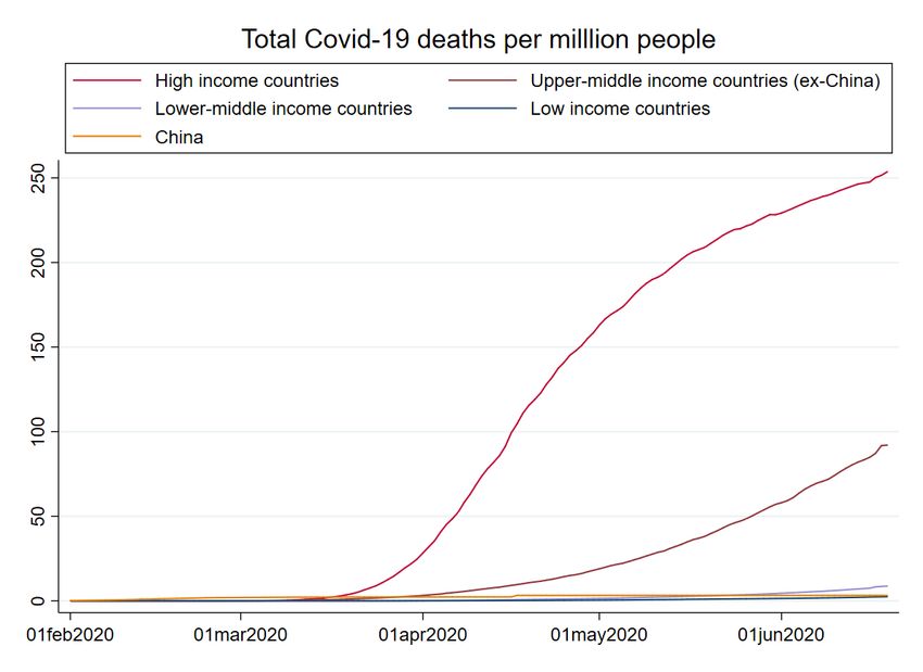
developing countries. However, due to the lack of mortality times series, “excess deaths” cannot
 be computed for most developing countries. In addition, the interpretation of “excess deaths” is
 not clear: such deaths capture both the direct mortality effects of COVID-19, and the indirect
 effects due for example to the disruption of non-COVID health care services, the pandemic’s
 effects on mental disease and suicides, the increase (or decrease) of violence, the increase (or
 decrease) of car accidents, etc. This may explain why South Africa, for instance, exhibits a
 negative number of excess deaths (suggesting that overall deaths have declined relative to earlier
 years), while official statistics report, as of June 20, 1,877 deaths attributed to COVID-19.
 A further concern, given that the pandemic is still ongoing, is whether the effects we document
 are due to countries being earlier or later on the curve. Mechanically, countries accumulate deaths
 as times passes, so countries that started having cases and deaths earlier in the year, will have a
 larger death toll. To account for this mechanical effect, we control for the time since the first
 death observed in each country through a square root function. This functional form is motivated
 by the pattern observed in several countries that seem to be toward the end of their infection and
 death curves (e.g., European countries)3. This approach seems adequate at present but would have
 to be revisited if countries faced a second wave of infections. One day, when the pandemic is
 over, one would want to run the above regression without controlling for this mechanical effect.
 Before reviewing the data and regression estimates, we graph the COVID-19 deaths per
 million people in Figure 2 by World Bank income group classification. To date, the picture in
 EMDEs seems to vindicate the optimists. Middle- and low-income countries seem to be on a very
 different curve than high-income countries. The graph clearly shows the earlier outbreak of the
 health crisis in high-income countries. But even accounting for this difference in timing, deaths in
 EMDEs are growing much more slowly over time. This is especially true for low income and
 lower-middle income countries. The curve for upper-middle income countries rises more steeply
 starting in May, reflecting the rising deaths in Latin America, especially in Brazil. That curve
 excludes China, which is shown separately, as the very low death rate in China would dominate
 the graph obfuscating the recent deaths in Latin America. Even taking this rise into account, it
 seems unlikely that middle- and low-income countries will catch up to high-income countries.

3
 We also experimented with a linear function with no significant impact on the results.
 12

Figure 2: Reported Covid-19 deaths per capita have been overwhelmingly concentrated in
 high income countries, though have recently been growing faster in upper-middle income
 countries excluding China
 Source: Our World in Data

 A different way to assess the raw differences between advanced and developing economies is
shown in Figure 3, which displays the raw correlation between deaths per million and national
income as of June 20. Deaths per million is strongly and positively correlated with per-capita
income. At present, the numbers across advanced and developing economies differ by orders of
magnitude. Almost every country with per capita income 1/16 of the United States has 1/16 the
deaths per million of the United States or fewer. Some specific examples may illustrate the
contrast: As of June 20, 2020, the U.S.A. had 369 deaths per 1 million people; France had 454;
Brazil: 236; Mexico: 161; South Africa: 32; Nigeria: 2; India: 10; Indonesia: 9; Philippines: 11;
Vietnam: 0. Such big differences across countries make it less likely that the positive relationship
between per capita deaths and per capita income reflects mismeasurement or data manipulation.
While infections and deaths in Brazil and Mexico are rising fast, so that the death rates in these

 13

countries may catch up to the U.S. eventually, for the rest of the countries, it would take a fast
acceleration of deaths for the pattern we document to be reversed. So far, such rapid acceleration
3-4 months after the first wave of infections seems unlikely given the patterns observed in
countries in Europe and Asia that were exposed earlier in the year, but it is possible that COVID
contagion and mortality follow a different pattern in lower income countries. And of course,
there is always the possibility of new waves, especially as countries are gradually opening up.

 Figure 3: National income and Covid-19 deaths per million are positively correlated
 Sources: Our World in Data. World Development Indicators
 Notes: Ordinary least squares fit shown as dashed line

A final note is that our regression makes no statement about indirect human costs of the pandemic,
because of lockdowns. Ray and Subramanian (2020) write eloquently on this topic in the context of
India stating “these lost lives, through violence, starvation, indebtedness and extreme stress, both
 14

psychological and physiological, are invisible, in the sense that they are—and will continue to
be—diffuse in space, time, cause and category.” These deaths are not accounted for in our
measure of COVID-19 deaths per million. One attempt to capture them would be to look at the
aforementioned “excess deaths” relative to previous monthly averages and to ask how many of
them can be explained by confirmed cases and how many reflect the indirect death toll of the
pandemic. Unfortunately, as noted earlier, the mortality time series required for this analysis are
not available systematically for EMDEs. Moreover, given existing concerns regarding
mismeasurement, it is not clear whether excess deaths that go beyond confirmed cases capture
undercounting of COVID deaths or the indirect death toll of the pandemic.

 I.B. Data
 Here we briefly review the data used, summary statistics of which are presented in Table 1.
COVID-19 deaths per million are from the “Our World in Data COVID-19 Dataset” of Roser et
al. (2020), and are compiled based on statistics released by the European Centre for Disease
Prevention and Control (ECDC). As noted earlier, our regressions include a function of
“days since first death” to account for the mechanical fact that countries accumulate more deaths
with time. This variable is set to zero for countries with no deaths to date. These data are also taken
from Roser at al. (2020).
 The “days since first death” function is meant to capture the mechanical effect of time on
deaths, but it may also proxy for a different channel. Late exposure to the virus may have been
the result of developing countries’ lower connectivity to the rest of the world. The late arrival of
the virus resulting from lower connectivity may have given developing countries extra time to
prepare and to take measures to contain the spread of the disease. To separate this channel from
the mechanical effect of time, we use three variables. First, we use two proxies for connectivity:
the “international flight arrivals per 1,000 people in December 2019 and January 2020” (also
broken down by origin, i.e., flights from China and flights from Schengen) and the “imports per
capita in 2019”. These measures are taken from Flight Radar 24 (a commercial flight tracking
service) and from COMTRADE respectively. We experimented with alternative measures (e.g.,
exports or the sum of imports and exports) with no difference in the results. Further, we use
information on the timing of the first response based on the Oxford COVID-19 Government
Response Tracker of Hale et al. (2020). Specifically, we use the time between the first time the

 15

government in a certain country acted related to COVID and the first death in that country to
measure the speediness of response. Note that for several countries, this variable takes negative
values as these countries acted before experiencing even a single death.
 In addition to the timing of the first public health response, we also investigate the strength of
the response, measured alternatively by the government response for “containment and health
response index” reported in Hale et al. (2020), and reductions in mobility around the work place and
public transit relative to early February, as reported by Google, LLC (2020). Further, we use a
“contract tracing comprehensiveness index,” which is reported by Oxford University as part of
their government health and containment response index; a value of 0 indicates no contact
tracing, and a value of 2 indicates contacts of all cases are traced, and a value of 1 indicates
limited tracing.
 GDP per capita is measured in constant 2010 United States dollars and taken from the WDI.
The health variables “population over age 70”, as well as “obesity”, and “smoking and diabetes”
prevalence is from the WHO. “PM2.5 air pollution” and “hospital beds per thousand people” are
from the WDI. “Population density of largest urban center” is as reported by the Global Human
Settlement Layer’s Urban Centre database.
 We include various measures of institutional capacity. Data on testing come from Roser et al.
(2020). Finally, we also examine measures of the extent to which either autocracy or democracy is
institutionalized in the country from the Polity IV database. According to these data monarchies such
as Saudi Arabia and Eswatini (previously Swaziland) have autocracy scores of 9 and 10, while
China has a 7. Countries scoring a 10 for democracy include Mongolia, Germany, while South
Africa has a 9 and the United States is ranked 8. All these countries are rated 0 for the extent of
institutionalized autocracy. The relationship between Covid-19 deaths and political and social
features of the state is studied by Bosancianu, Dionne, Hilbig, Humphreys, KC, Lieber and
Scacco (2020), though they do not include these indicators. We also include an index of statistical
capacity developed by the World Bank, ranging from 0-100, in order to test whether
measurement specifically can account for deaths per million. For this index, which is not
available for high income countries, we set the value for all high income countries equal to the
maximum, 97, so that the index has the greatest possible potential to explain the association
between income and deaths per million.
 Actual rainfall for February to May 2020 is measured using data from the National Oceanic

 16

Atmospheric Administration. Precipitation for each country is measured in average millimeters per
day using the Climate Prediction Center Merged Analysis of Precipitation (CMAP) data-set, which
reports values on a 2.5x2.5 degree grid obtained by combining satellite estimates and gauge data
(Xie and Arkin, 1997). Values on the grid are averaged within administrative boundaries. 4 As an
alternative to using data on temperature, we use “distance to equator” as a proxy for
weather/climate; this variable is measured in degrees latitude from the centroid of the national
administrative boundaries reported by Natural Earth.
 Finally, it has been hypothesized that exposure to prior epidemics may have conferred to
some developing countries “trained immunity5.” To investigate this hypothesis, we use
information on prior SARS-CoV-1 and MERS-CoV infections. Locations of non-imported
SARS-CoV-1 are Canada, China, Mongolia, the Philippines, Singapore and Vietnam, as reported
by the WHO. Locations of non-imported MERS are in Bahrain, Iran, Jordan, Kuwait, Lebanon,
Oman, Saudi Arabia, United Arab Emirates and Yemen, as reported by the WHO.

 4
 Country values are calculated in two steps. First, inverse distance weighted interpolation is used to
generate a 1x1 degree grid of monthly rainfall values; a power coefficient equal to 5 is applied to the distance
measure, so that interpolated points reflect mainly the nearest values. This step is necessary because the
boundaries of several small countries do not contain any point on the original 2.5x2.5 grid. Second, rainfall
on all points within the 1x1 degree grid are averaged within the administrative boundaries of each country.
 5
 Netea et al (2020) define “trained immunity” as a biological process, by which activation of the innate
immune system can result in enhanced responsiveness to subsequent triggers - a de facto innate immune
memory.
 17

(1) (2) (3) (4) (5)
 VARIABLES N mean sd min max
 Confirmed Covid-19 deaths per million people 197 59 147 0 1,238
 Days since first death (=0 if no deaths) 197 76 32 0 161
 Real GDP per capita (2010 USD) 189 17,699 26,542 211 195,880
 Population over age 70 (%) 182 6.1 4.8 0.7 22
 Obesity prevalence (% of adults) 177 18 8.9 2.1 38
 Smoking prevalence (% of adults) 139 21 9.5 2 46
 Diabetes prevalence (% of adults) 193 8.0 4.2 1 22
 PM2.5 air pollution (µg/cm3) 183 28 19 5.9 100
 Hospital beds per thousand people 185 3.1 2.8 0.1 19
 Dec., Jan. int'l flight arrivals per 1,000 people 197 1.3 2.8 0.0002 18
 Dec., Jan. flight arrivals from China per 1,000 people 197 0.02 0.05 0.000005 0.3
 Dec., Jan. flight arrivals from Schengen area per 1,000 people 197 0.3 1.0 0.00001 6.7
 Imports per capita (USD) 162 5,983 8,775 71 65,708
 Imports from China per capita (USD) 161 561 936 6.0 8,802
 Imports from Schengen area per capita (USD) 162 8,367 12,815 81 74,585
 Days before first death that action is taken 169 53 34 -79 171
 Containment and health response 4 weeks after first death (0-100) 151 75 14 17 100
 Workplace mobility decline 4 weeks after first death (%) 121 -45 20 -90 5
 Public transit mobility decline 4 weeks after first death (%) 121 -57 19 -93 -5
 General cancellation of public events 4 weeks after first death (=1) 152 0.9 0.3 0 1
 Containment and health response 90 days after first death (0-100) 37 70 13 46 94
 Population per km2 in largest urban center 173 6,511 3,397 1,172 19,843
 Persons per household 144 3.9 1.4 2.1 8.7
 Covid-19 tests per 1,000 people 83 42 50 0.5 267
 Positive test ratio (%) 83 9.3 17 0.1 117
 Contact tracing comprehensiveness index (0-2) 151 1.3 0.7 0 2
 Statistical capacity (0-100) 195 75 19 27 97
 Institutionalized democracy (0-10) 148 6.0 3.7 0 10
 Institutionalized autocracy (0-10) 148 1.6 2.7 0 10
 Feb. precipitation (mm/day) 197 2.8 2.4 0.03 13
 Mar. precipitation (mm/day) 197 2.4 2.1 0.02 12
 Apr. precipitation (mm/day) 197 2.6 2.2 0.03 13
 May precipitation (mm/day) 197 3.0 2.7 0.06 19
 Non-imported cases of SARS-CoV-1 (=1) 197 0.03 0.2 0 1
 Non-imported cases of MERS-CoV (=1) 197 0.05 0.2 0 1

 Table 1: Summary statistics
I.C. Regression Results
 Table 2 reports the results of estimating several specifications of Equation (1) using ordinary
least squares. Additional specifications are reported in the Appendix. Before taking logs of
deaths per million we have added 0.0219 to the value for 20 countries with zero confirmed deaths,
so that they are not dropped from estimation, treating them as if they experience 2.9 deaths per 100
million people. This exact number was selected so these countries have exactly 1/(4 × 4096) the
deaths per million of the United States, implying the Y-axis tick on which they sit in Figure 3 is
 18

evenly spaced from the others above it. The full sample includes 189 observations of deaths per
million and GDP per capita.
 We present this regression with the important qualifier that the dependent variable (deaths per
million) continually changes, and hence the results may change in the future. Column (1) reports
the coefficient on the log of per capita income in the absence of any additional explanatory
variables Xi. Here the coefficient ρ = 0.878 (s.e. = 0.102), suggests that for a 1 percent increase in
income there is approximately a 0.9 percent increase in deaths per million, corresponding to the
linear fit displayed graphically in Figure 3. Further, the R-squared (which has been adjusted for the
number of explanatory terms in the model) is 0.24, indicating that roughly one fourth of the
variation in deaths per million is explained by income.
 We now add additional variables sequentially to unpack this relationship. In Column (2) we add
the square root of days since first death (which is set to zero for those 21 countries with zero
confirmed deaths) to account for the mechanical effect that countries later in the pandemic will
have accumulated more deaths. The adjusted R-squared rises to 0.677, suggesting timing of arrival
explains a substantial part of the overall variation in deaths. The coefficient ρ = 0.599 (s.e. = 0.077)
has fallen, consistent with the fact that EMDEs experienced their first death later, but remains
statistically significant below 1 percent and is sizable in magnitude.
 In Column (3) we add two risk factors for severe Covid-19 illness: the share of the population
over age 70 and obesity prevalence. Notably, since accurate body mass index data are difficult to
come by for representative samples of the confirmed cases within countries (Lighter et al., 2020),
our cross country regression presents a novel opportunity to investigate the contribution of obesity
to COVID-mortality. The element of β corresponding to the coefficient on the age variable is
positive and significant, equal to 0.079 (s.e. = 0.028), suggesting that for a 1 percentage point increase
in the population over 70, deaths per million increase by 0.8 of a percent. The element of β
corresponding to the coefficient on obesity is also positive and significant, equal to 0.060 (s.e. =
0.019), suggesting that for a 1 percentage point increase in obesity prevalence, deaths per million
increase by 0.6 of a percent, an effect roughly three quarters of the effect of the size of the population
over 70. The coefficient ρ = 0.186 (s.e. = 0.121) falls substantially relative to the previous
specifications and becomes statistically insignificant, suggesting that the high initial correlation
between income and deaths can be explained alone by two risk factors for severe illness (age and
obesity) and the time of virus’ arrival.

 19

VARIABLES (1) (2) (3) (4) (5) (6) (7) (8) (9) (10)

Ln(real GDP per capita) 0.878*** 0.599*** 0.186 0.677*** 0.734*** 0.163 0.317** 0.323** 0.320** 0.340**
 (0.102) (0.077) (0.121) (0.087) (0.118) (0.115) (0.138) (0.139) (0.135) (0.131)
Square root of days since first death 0.622*** 0.566*** 0.512*** 0.179 0.488*** 0.448*** 0.440*** 0.450*** 0.437***
(=0 if no deaths) (0.030) (0.033) (0.062) (0.233) (0.055) (0.057) (0.061) (0.058) (0.061)
Population over age 70 (%) 0.079*** 0.102*** 0.118*** 0.129*** 0.095** 0.087**
 (0.028) (0.028) (0.031) (0.032) (0.041) (0.043)
Obesity prevalence (% of adults) 0.060*** 0.071*** 0.075*** 0.079*** 0.070*** 0.072***
 (0.019) (0.019) (0.020) (0.020) (0.021) (0.020)
Days before first death that action is taken -0.008 -0.010 -0.004 -0.003 -0.004 -0.003 -0.005
 (0.005) (0.006) (0.004) (0.004) (0.004) (0.004) (0.004)
Response stringency 4 weeks after first death (0-100) -0.006
 (0.012)
Workplace mobility decline 4 weeks after first death (%) -0.038***
 (0.012)
Public transit mobility decline 4 weeks after first death (%) 0.020
 (0.016)
Ln(Population per km2 in largest urban center) 0.916*** 0.986*** 0.917*** 1.030***
 (0.310) (0.321) (0.311) (0.317)
Feb. precipitation (mm/day) -0.105 -0.115
 (0.082) (0.082)
Mar. precipitation (mm/day) 0.265*** 0.275***
 (0.097) (0.098)
Apr. precipitation (mm/day) -0.130 -0.106
 (0.105) (0.105)
May precipitation (mm/day) 0.050 0.073
 (0.056) (0.061)
Distance to equator (degrees latitude) 0.010 0.018
 (0.010) (0.012)
Constant -5.756*** -8.447*** -5.988*** -7.868*** -5.245** -5.304*** -14.461*** -15.307*** -14.527*** -16.016***
 (0.907) (0.654) (0.812) (0.866) (2.257) (0.868) (3.168) (3.280) (3.155) (3.213)
Observations 189 189 172 166 115 157 155 155 155 155
Adjusted R-squared 0.239 0.677 0.673 0.662 0.409 0.684 0.679 0.687 0.679 0.691

 Table 2: Regression of (log) COVID-19 deaths per million people on country covariates
 Notes: Standard errors are robust to heteroskedasticity. ***p

In the Appendix table A2, we explore specifications that include additional health covariates
(smoking prevalence; diabetes prevalence; as well as a measure of particulate matter pollution since
pollution may increase asthma prevalence). We consistently find no statistically significant effect of
these variables on deaths per million, once age and obesity were controlled for. Moreover, they often
have counterintuitive signs (column 1 in table A2). Health care capacity (as measured by hospital
beds per 1,000 people) is also insignificant (column 2 in table A2), but with a negative sign, as
expected. We also consider a specification that controls for the hypothesized “trained immunity”
effect through dummies indicating countries had non-imported cases of SARS-CoV-1 and MERS-
CoV (column 4 in table A2). We find a large, negative, and statistically effect of SARS-CoV-1 on
deaths per million. The coefficient on MERS-CoV is negative, but not significant. Importantly, the
inclusion of these covariates has no effect on the remaining coefficients, and on the income
coefficient – hence, it does not help explain the positive correlation between deaths and income. The
SARS-CoV-1 dummy acts as a proxy for countries in East Asia, which have much lower death rates,
and may therefore also capture factors other than trained immunity. For this reason, we do not include
it in other specifications. In general, we avoid using country dummies (or variables that effectively act
as country dummies), since we estimate a cross-country regression, and country dummies wipe out
relevant variation in our covariates.
 In Columns (4) and (5) of Table 1, we omit the two risk factors (age and obesity) and control
instead for the public health policy response. In Column (4), we add just one variable that measures
the days before first death that action is taken by the government on the public health response.
Whereas before we had been controlling for when the virus arrived in the country (through days
since first death), we are now also controlling for the time at which the government responded. As
expected, the coefficient on this variable is negative, but not statistically significant at
conventional levels. The coefficient ρ = 0.677 (s.e. = 0.087) has risen and is again statistically
significant. Conditional the timing of first death and government action, there is still a strong
positive correlation between income and deaths per million. In Column (5), we examine whether the
strength of lockdown measures mattered in addition to the timing of first action, by adding both
the value of the “containment and health response index” and observed changes in mobility from
workplaces and on public transit. Note that because the mobility reports are not available for all
countries in our sample, we lose some observations, and hence columns (4) and (5) are not
directly comparable.
 21

Nevertheless, the results in Column (5) provide some useful insights. The policy response
variables are all insignificant (both in Column 5 and in additional specifications in Appendix
table A2 that use alternative time windows or subcomponents of the stringency index). However,
the decline in workplace mobility is found to have a negative and significant impact on deaths per
capita. Interestingly, the inclusion of mobility controls increases the correlation between deaths
per capita and income. A recent piece by Maire (2020) may explain why. Maire finds that low
income and lower-middle income countries had lower compliance (i.e., decline in mobility)
conditional on the policy stringency index than the rest of the countries. Hence, it does not appear
that developing countries have contained the death toll because of lower mobility – in contrast, it
seems that they have a lower death rate despite not reducing mobility.
 In Columns (6) to (10), we reintroduce the two risk factors, age and obesity, that were shown
to have a significant impact on cross-country differences. Given that mobility reports are not
available for all countries in our sample (and that they do not appear to explain why developing
countries have lower death rates anyway), we omit them from these specifications, but always
include the early action control (timing of first policy response). The latter turns out to be always
insignificant, though it has the expected negative sign. Columns (7) to (10) introduce one
population additional variable, the density in a country’s largest urban center. This variable has a
large positive and significant effect in all specifications as expected. Further, average household
size does not significantly predict death rates conditional on the density of the largest urban center
(column 3 in Appendix table A2). Interestingly, however, once population density is introduced,
the correlation between deaths and income (that had become small and insignificant once age and
obesity were controlled for) reappears, though it is substantially lower than in the initial
specifications that do not control for risk factors. This suggests that once again, developing
countries do not have fewer deaths because they have fewer dense cities; they have fewer deaths
despite having some of the densest cities in the world 6.
 In columns (8) to (10), we add controls for weather/climate. Among them, the only one that is
consistently significant is precipitation in March that enters with a positive sign. This is likely
because several South American countries with high death rates also experienced substantial
precipitation in March, namely Brazil, Ecuador and Peru. Distance to equator which proxies for

6
 Out of the top 10 for population density cities in the world, 8 are in developing countries. Four of them are in the
Philippines alone.
 22

warm temperature and humidity (among many other things) is not statistically significant.
Overall, we do not find support for the hypothesis that warm climate might slow the virus or even
suppress it.
 In all specifications, the magnitudes and signs of age and obesity remain robust. So does the
correlation of deaths with income. This correlation is not significantly different from zero if we
do not control for population density of the largest urban sector. It is consistently around 0.32 (so
about one third of the original correlation without any controls) once we condition on population
density of the largest city. Population density clearly matters. But it does not explain the
difference between advanced and developing economies.
 The Appendix tables report additional robustness checks. The effects of age, obesity, and
population density of the largest urban center remain robust. In Table A1, we include various
controls for connectivity. The controls are mostly insignificant, except for flight arrivals from
China, which proxies for China (as this measure includes domestic flights in China). Not
surprisingly, the associated coefficient is negative and significant as China has had a lower death
rate. Similarly, in one specification in Column (4), flight arrivals from the Schengen area have a
large (positive) impact on death, but this variable likely proxies for European countries, which
have had a particularly high death toll. For the reasons given earlier, we avoid variables that act
as country dummies. Notably, the inclusion of the connectivity measures does not affect either
the income or the time since first death variables. In Table A2 we consider further covariates. In
Column (5), we add the (log) number of tests per thousand and the positive test rate.
Unfortunately, the number of observations drops to 78, so we cannot draw any definitive
conclusions based on this specification. But interestingly, once the testing measures are included,
the coefficient on income drops and is no longer significantly different from zero (even when
population density is controlled for). The coefficients on both testing measures are positive and
significant. Given that testing is not random, the interpretation of these coefficients is not
straightforward. But if we interpret the test positive rate as a measure of the capacity of the
testing system (rather than a measure of the infections rate), then the positive coefficient supports
the view that higher testing capacity (reflected in a lower testing ratio) is associated with fewer
deaths. As noted earlier, many low income countries have some of the most comprehensive
testing programs of the world, given their disease burden. The results in Column (5) of table A2
suggest that the lower death rates of EMDEs can be attributed to younger populations, limited
 23

obesity, and higher testing capacity. Column (9) in table A2 includes controls for the regime type.
Though the coefficient on democracy is positive, and the coefficient on autocracy is negative,
suggesting democracy may have made controlling the disease harder, as some have speculated for
instance in the context of the United States, though these effects are not statistically significant.

 I.D. Tentative Conclusions
 Based on these preliminary results, it appears that a large part of the positive correlation between
income and deaths per million is due to demographics and health covariates, in particular the age
distribution and obesity. As of now, these covariates seem to explain almost all the difference
between advanced and developing economies.
 We conclude, tentatively, that the public health care crisis in EMDEs has not be as severe as
initially feared. No matter what the reason for this is, it is good news. It means that fewer lives
were lost. It also means that – to the extent this pattern is not reversed in the future – developing
countries may be able to lift strict containment measures and focus on the economic situation, to
which we turn in the next section.

 II. The Economic Crisis
 II.A. Short and Medium Run
 EMDEs could face years of economic hardship due both to suppression measures, the
continued duration of which is uncertain, and to spillover effects from a global recession. In
advanced economies, the hope was that once countries brought the public health crisis under
control, they would manage the economic crisis. For smaller economies especially, the decline in
commodity export revenues and remittances from migrants to advanced economies implies that
the economic effects could be grave, even if they manage to control the virus.
 We structure the discussion of the short- and medium-run economic effects in three parts. We
first discuss external vulnerabilities focusing on financial markets. Next, we discuss preliminary
evidence on the effects of countries’ own containment policies. Finally, we offer some thoughts
on policy implications.

 External Vulnerabilities
 Given limited availability of data on macroeconomic variables at this early moment, we start
 24