The Eocene-Oligocene transition: a review of marine and terrestrial proxy data, models and model-data comparisons
←
→
Page content transcription
If your browser does not render page correctly, please read the page content below
Clim. Past, 17, 269–315, 2021
https://doi.org/10.5194/cp-17-269-2021
© Author(s) 2021. This work is distributed under
the Creative Commons Attribution 4.0 License.

The Eocene–Oligocene transition: a review of marine and
terrestrial proxy data, models and model–data comparisons
David K. Hutchinson1 , Helen K. Coxall1 , Daniel J. Lunt2 , Margret Steinthorsdottir1,3 , Agatha M. de Boer1 ,
Michiel Baatsen4 , Anna von der Heydt4,5 , Matthew Huber6 , Alan T. Kennedy-Asser2 , Lutz Kunzmann7 ,
Jean-Baptiste Ladant8 , Caroline H. Lear9 , Karolin Moraweck7 , Paul N. Pearson9 , Emanuela Piga9 ,
Matthew J. Pound10 , Ulrich Salzmann10 , Howie D. Scher11 , Willem P. Sijp12 , Kasia K. Śliwińska13 , Paul A. Wilson14 ,
and Zhongshi Zhang15,16
1 Department    of Geological Sciences and Bolin Centre for Climate Research, Stockholm University, Stockholm, Sweden
2 School  of Geographical Sciences, University of Bristol, Bristol, UK
3 Department of Palaeobiology, Swedish Museum of Natural History, Stockholm, Sweden
4 Institute for Marine and Atmospheric Research, Department of Physics, Utrecht University, Utrecht, the Netherlands
5 Centre for Complex Systems Studies, Utrecht University, Utrecht, the Netherlands
6 Department of Earth, Atmospheric, and Planetary Sciences, Purdue University, West Lafayette, USA
7 Senckenberg Natural History Collections, Dresden, Germany
8 Department of Earth and Environmental Sciences, University of Michigan, Ann Arbor, USA
9 School of Earth and Ocean Sciences, Cardiff University, Cardiff, UK
10 Department of Geography and Environmental Sciences, Northumbria University, Newcastle upon Tyne, UK
11 School of the Earth, Ocean and Environment, University of South Carolina, Columbia SC, USA
12 Climate Change Research Centre, University of New South Wales, Sydney, Australia
13 Department of Stratigraphy, Geological Survey of Denmark and Greenland (GEUS), Copenhagen, Denmark
14 University of Southampton, National Oceanography Centre, Southampton, UK
15 Department of Atmospheric Science, China University of Geoscience, Wuhan, China
16 NORCE Research and Bjerknes Centre for Climate Research, Bergen, Norway

Correspondence: David K. Hutchinson (david.hutchinson@geo.su.se)

Received: 3 May 2020 – Discussion started: 18 May 2020
Revised: 17 November 2020 – Accepted: 18 November 2020 – Published: 28 January 2021

Abstract. The Eocene–Oligocene transition (EOT) was a            thesise proxy evidence of palaeogeography, temperature, ice
climate shift from a largely ice-free greenhouse world to        sheets, ocean circulation and CO2 change from the marine
an icehouse climate, involving the first major glaciation of     and terrestrial realms. Furthermore, we quantitatively com-
Antarctica and global cooling occurring ∼ 34 million years       pare proxy records of change to an ensemble of climate
ago (Ma) and lasting ∼ 790 kyr. The change is marked by a        model simulations of temperature change across the EOT.
global shift in deep-sea δ 18 O representing a combination of    The simulations compare three forcing mechanisms across
deep-ocean cooling and growth in land ice volume. At the         the EOT: CO2 decrease, palaeogeographic changes and ice
same time, multiple independent proxies for ocean tempera-       sheet growth. Our model ensemble results demonstrate the
ture indicate sea surface cooling, and major changes in global   need for a global cooling mechanism beyond the imposition
fauna and flora record a shift toward more cold-climate-         of an ice sheet or palaeogeographic changes. We find that
adapted species. The two principal suggested explanations of     CO2 forcing involving a large decrease in CO2 of ca. 40 %
this transition are a decline in atmospheric CO2 and changes     (∼ 325 ppm drop) provides the best fit to the available proxy
to ocean gateways, while orbital forcing likely influenced the   evidence, with ice sheet and palaeogeographic changes play-
precise timing of the glaciation. Here we review and syn-        ing a secondary role. While this large decrease is consistent

Published by Copernicus Publications on behalf of the European Geosciences Union.
270                                                                D. K. Hutchinson et al.: The Eocene–Oligocene transition

with some CO2 proxy records (the extreme endmember of              proaches and highlight areas for future work. We then com-
decrease), the positive feedback mechanisms on ice growth          bine and synthesise the observational and modelling aspects
are so strong that a modest CO2 decrease beyond a critical         of the literature in a model–data intercomparison of the avail-
threshold for ice sheet initiation is well capable of triggering   able models of the EOT. This approach allows us to assess
rapid ice sheet growth. Thus, the amplitude of CO2 decrease        the relative effectiveness of the three modelled mechanisms
signalled by our data–model comparison should be consid-           in explaining the EOT observations.
ered an upper estimate and perhaps artificially large, not least      The paper is structured as follows: Sect. 1.2 defines the
because the current generation of climate models do not in-        chronology of events around the EOT and clarifies the ter-
clude dynamic ice sheets and in some cases may be under-           minology of associated events, transitions and intervals,
sensitive to CO2 forcing. The model ensemble also cannot           thereby setting the framework for the rest of the review. Sec-
exclude the possibility that palaeogeographic changes could        tion 2 reviews our understanding of palaeogeographic change
have triggered a reduction in CO2 .                                across the EOT and discusses proxy evidence for changes in
                                                                   ocean circulation and ice sheets. Section 3 synthesises ma-
                                                                   rine proxy evidence for sea surface temperatures (SSTs) and
                                                                   deep-ocean temperature change. Section 4 synthesises terres-
1     Introduction
                                                                   trial proxy evidence for continental temperature change, with
1.1    Scope of review                                             a focus on pollen-based reconstructions. Section 5 presents
                                                                   estimates of CO2 forcing across the EOT, from geochemical
Since the last major review of the Eocene–Oligocene transi-        and stomatal-based proxies. Section 6 qualitatively reviews
tion (EOT; Coxall and Pearson, 2007) the fields of palaeo-         previous modelling work, and Sect. 7 provides a new quan-
ceanography and palaeoclimatology have advanced consid-            titative intercomparison of previous modelling studies, with
erably. New proxy techniques, drilling and field archives of       a focus on model–data comparisons to elucidate the relative
Cenozoic (66 Ma to present) climates, have expanded global         importance of different forcings across the EOT. Section 8
coverage and added increasingly detailed views of past cli-        provides a brief conclusion.
mate patterns, forcings and feedbacks. From a broad perspec-
tive, statistical interrogation of an astronomically dated, con-   1.2   Terminology of the Eocene–Oligocene transition
tinuous composite of benthic foraminifera isotope records
confirms that the EOT is the most prominent climate tran-          Palaeontological evidence has long established Eocene (56 to
sition of the whole Cenozoic and suggests that the polar ice       34 Ma) warmth in comparison to a long-term Cenozoic cool-
sheets that ensued seem to play a critical role in determin-       ing trend (Lyell and Deshayes, 1830, p. 99–100). As modern
ing the predictability of Earth’s climatological response to       stratigraphic records improved, a prominent step in that cool-
astronomical forcing (Westerhold et al., 2020). New proxy          ing towards the end of the Eocene began to be resolved. This
records capture near- and far-field signals of the onset of        became evident in early oxygen isotope records (δ 18 O) de-
Antarctic glaciation. Meanwhile, efforts to simulate the onset     rived from deep-sea benthic foraminifera, which show an iso-
of the Cenozoic “icehouse”, using the latest and most sophis-      tope shift towards higher δ 18 O values (Kennett and Shackle-
ticated climate models, have also progressed. Here we review       ton, 1976; Shackleton and Kennett, 1975), which was subse-
both observations and the results of modelling experiments         quently attributed to a combination of continental ice growth
of the EOT. From the marine realm, we review records of sea        and cooling (Lear et al., 2008). In the 1980s the search was
surface temperature, as well as deep-sea time series of the        on for a suitable global stratotype section and point (GSSP)
temperature and land ice proxy δ 18 O and carbon cycle proxy       to define the Eocene–Oligocene boundary (EOB). Much of
δ 13 C. From the terrestrial realm we cover plant records and      the evidence was brought together in an important synthe-
biogeochemical proxies of temperature, CO2 and vegetation          sis edited by Pomerol and Premoli Silva (1986). The GSSP
change. We summarise the main evidence of temperature,             was eventually fixed at the Massignano outcrop section in
glaciation and carbon cycle perturbations and constraints on       the Marche region of Italy in 1992 (Premoli Silva and Jenk-
the terrestrial ice extent during the EOT, and review indica-      ins, 1993) at the 19.0 m mark which corresponds to the ex-
tors of ocean circulation change and deep-water formation,         tinction of the planktonic foraminifer family Hantkeninidae
including how these changes reconcile with palaeogeogra-           (Coccione, 1988; Nocchi et al., 1986). By the conventions of
phy, in particular, ocean gateway effects.                         stratigraphy, Massignano is the only place where the EOB is
   Finally, we synthesise existing model experiments that          defined unambiguously; everywhere else the EOB must be
test three major proposed mechanisms driving the EOT:              correlated to it, whether by biostratigraphy, magnetostratig-
(i) palaeogeography changes, (ii) greenhouse forcing and           raphy, isotope stratigraphy or other methods.
(iii) ice sheet forcing upon climate. We highlight what has           Coxall and Pearson (2007, p. 352) described the EOT as
been achieved from these modelling studies to illuminate           “a phase of accelerated climatic and biotic change lasting
each of these mechanisms and explain various aspects of            500 kyr that began before and ended after the E/O bound-
the observations. We also discuss the limitations of these ap-     ary”. Recognising and applying this in practice turns out

Clim. Past, 17, 269–315, 2021                                                          https://doi.org/10.5194/cp-17-269-2021
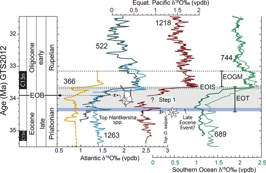
D. K. Hutchinson et al.: The Eocene–Oligocene transition                                                                                  271

Figure 1. Oxygen stable isotope and chronostratigraphic characteristics of the Eocene–Oligocene transition (EOT) from deep marine records
and EOT terminology on the GTS2012 timescale. Benthic foraminiferal δ 18 O from six deep-sea drill holes are shown: tropical Atlantic Site
366, South Atlantic sites 522 and 1263 (Zachos et al., 1996; Langton et al., 2016); Southern Ocean sites 744 and 689 (Zachos et al., 1996;
Diester-Haass and Zahn, 1996) and equatorial Pacific Site 1218 (Coxall and Wilson 2011). Due to different sample resolutions, running
means are applied using a three-point filter for sites 522, 689 and 1263; five-point filter for sites 366 and 744; and a seven-point filter for
Site 1218. Timescale conversions were made by aligning common magnetostratigraphic tie points. The EOT is defined as a ca. 790 kyr long
phase of accelerated climatic and biotic change that began before and ended after the Eocene–Oligocene boundary (EOB) (after Coxall and
Pearson, 2007). It is bounded at the base by the “top” D. saipanensis nannofossil extinction event and above by the EOIS-δ 18 O maximum.
Benthic data are all Cibicidoides spp. or “Cibs. equivalent” and have not been adjusted to seawater equilibrium values. “Step 1” comprises
a modest δ 18 O increase linked to ocean cooling (Lear et al., 2008; Bohaty et al., 2012). The “top Hantkenina spp.” marker corresponds to
the position of this extinction event at DSDP Site 522 (including sampling bracket) with respect to the corresponding Site 522 δ 18 O curve.
That it coincides with the published calibrated age of this event (33.9 Myr) is entirely independent. The “late Eocene event” δ 18 O maximum
(after Katz et al., 2008) may represent a failed glaciation.

to be problematic due to variability in the pattern of δ 18 O             graphic tool. These also show a correlatable stepped pattern
between records and on different timescales. Widespread                   of increase across the EOT, although in detail δ 18 O and δ 13 C
records now show the positive δ 18 O shift with increasing                are not synchronous (Coxall et al., 2005; Zachos et al., 1996)
detail. A high-resolution record from Ocean Drilling Pro-                 and further complications arise in correlation to other sites
gram (ODP) Site 1218 in the Pacific Ocean revealed two                    (Coxall and Wilson, 2011). In attempting to synthesise the
δ 18 O and δ 13 C “steps” separated by a more stable “plateau             pattern across multiple sites, we suggest that attempts to de-
interval” (Coxall et al., 2005; Coxall and Wilson, 2011). The             fine and correlate an initial “Step 1” are premature at this
EOT brackets these isotopic steps with the EOB falling in                 point and should await better-resolved records. Nonetheless,
the plateau between them (Coxall and Pearson, 2007; Cox-                  we maintain a tentative Step 1 in our terminology because
all and Wilson, 2011; Dunkley Jones et al., 2008; Pearson et              it is important for differentiating phases of cooling vs ice
al., 2008). However, while two-step δ 18 O patterns have now              growth during the EOT.
been interpreted in other deep-sea records, thus far largely                 Settling on a consistent terminology for other features of
from the Southern Hemisphere (Fig. 1) (Bohaty et al., 2012;               the EOT is also problematic because usage of certain terms
Borrelli et al., 2014; Coxall and Wilson, 2011; Langton et                has changed through time. In order to clarify the definition
al., 2016; Pearson et al., 2008; Wade et al., 2012; Zachos et             of two key stratigraphic features, we recommend using the
al., 1996), there is often ambiguity in their identification. In          following terms: (i) for the basal Oligocene δ 18 O increase
particular, while the second δ 18 O step, “Step 2” of Coxall              we suggest the term “earliest Oligocene oxygen isotope step”
and Pearson (2007), is an abrupt and readily correlated fea-              (EOIS) to denote the large isotope step that occurs well after
ture, the first step (Step 1 of Pearson et al., 2008; EOT-1 of            the EOB and within the lower part of chron C13n (Fig. 1);
Katz et al., 2008) is often less prominent than at Site 1218              (ii) we suggest the term “early Oligocene glacial maximum”
(Fig. 1). Furthermore, some records have been interpreted to              (EOGM; Liu et al., 2004; Fig. 1) to denote the peak-to-peak
show more than two δ 18 O steps (e.g. Katz et al., 2008). Ben-            isotope stratigraphic interval, corresponding to most of chron
thic δ 13 C records provide a powerful complementary strati-              C13n (starting at the top of the EOIS). Other terms for these

https://doi.org/10.5194/cp-17-269-2021                                                                    Clim. Past, 17, 269–315, 2021
272                                                                            D. K. Hutchinson et al.: The Eocene–Oligocene transition

Table 1. Summary of Eocene Oligocene terminology and approximate timings of events, as interpreted at the time of writing. Timescales
referred to are GTS2012 (Gradstein et al., 2012) and CK95 (Cande and Kent, 1995).

 Event          Abbr.     Definition                 Correlation                Timing                       Comment                  Also known as
 Early          EOGM      Period of cold cli-        Peak-to-peak     δ 18 O    33.65 to ∼ 33.16 Ma,         Defined by Liu et        Oi-1 (Zachos et al.,
 Oligocene                mate/glaciation in the     stratigraphic interval     ∼ 490 kyr duration           al. (2004). The end      1996) including the
 glacial                  early Oligocene cor-       starting at the top of                                  of the EOGM may          separate δ 18 O maxima
 maximum                  responding to most of      the EOIS & extending                                    correspond to a          Oi-1a and Oi-1b
                          magnetic chron C13n        to another peak around                                  second δ 18 O peak,
                                                     the top of C13n                                         sometimes referred
                                                                                                             to as Oi-1b
 Chron C13n     C13n      Interval of normal         Between specific mag-      33.705–33.157 Ma             Very useful for corre-   –
                          magnetic polarity in       netic reversals            (GTS2012)                    lation & dating when
                          the early Oligocene                                                                available
                          broadly     correlative
                          with the EOGM
 Eocene–        EOT       A phase of acceler-        Stratigraphic interval     Start: “top” D. saipa-       Definition    revised    –
 Oligocene                ated climatic & biotic     between the extinction     nensis extinction event;     here after Coxall and
 transition               change that began be-      of Discoaster saipa-       end: end of EOIS δ 18 O      Pearson (2007)
                          fore and ended after the   nensis & the top of the    maximum event;
                          EOB                        EOIS                       duration ∼ 790 kyr
 Earliest       EOIS      Short period of rapid      Stratigraphically above    The peak is at               Herein defined as        The “Oi1 event” “... at
 Oligocene                δ 18 O increase (0.7 ‰     the EOB & within the       ∼ 33.65 Ma                   the end of the EOT       the base of Zone Oi1”,
 oxygen                   or more) that occurred     lowermost part of chron    (GTS2012);                   and the start of the     Miller et al. (1991);
 isotope step             well after the EOB &       C13n                       duration ∼ 40 kyr            EOGM                     Oi-1a of Zachos et
                          within the lower part of                                                                                    al. (1996)
                          chron C13n
 Eocene         EOB       The       stratigraphic    Denoted by the extinc-     33.9 Ma (GTS2012),           –                        Base Oligocene epoch;
 Oligocene                boundary between the       tion of the planktonic     33.7 Ma (CK95)                                        base Rupelian stage
 boundary                 Eocene and Oligocene       foraminifera Hantken-
                          epochs defined at the      inain the marine realm
                          Massignano GSSP
 Step 1         –         The first-step increase    Harder to identify &       ∼ 34.15 Ma;                  –                        EOT-1,        Katz  et
                          in δ 18 O occurring        correlate than the EOIS    duration ∼ 40 kyr.                                    al. (2008); “precur-
                          shortly before the EOB                                                                                      sor glaciation”, Scher
                          in some records                                                                                             et al. (2011)
 Late Eocene    –         A transient late Eocene    Transient interval of      Onset is coincident          Defined by Katz et       –
 event                    cool or glacial event      positive δ 18 O seen in    (within 80 kyr analyt-       al. (2008);
                          near the start of the      some records               ical error; Coxall et        defines the start of
                          EOT                                                   al., 2005) with the D.       the EOT as defined
                                                                                saipanensis extinction       herein
                                                                                (34.44 Ma) at Site 1218
 Priabonian     PrOM      A transient late Eocene    Transient interval of      ∼ 37.3 Ma;   duration        Defined by Scher et      –
 oxygen                   cool or glacial event      positive δ 18 O seen       ∼ 140 kyr, tentatively       al. (2014)
 isotope                                             in some records well       placed within chron
 maximum                                             below the EOT              C17n.1n

features have been used inconsistently in the literature (Ta-                  in Coxall and Pearson, 2007, p. 352). The terms “Oi-1a” and
ble 1). For example, the term “Oi-1” was originally defined                    “Oi-1b”, originally defined by Zachos et al. (1996) as “... two
(at DSDP Site 522) by Miller et al. (1991) as an isotope                       distinct, 100 to 150 kyr long glacial maxima ... separated by
stratigraphic “zone” between one oxygen isotope peak and                       an ‘interglacial”’, have also been inconsistently applied in the
another, corresponding to a duration of several millions of                    literature and are now arguably an impediment to clear com-
years. Here there was a distinction between the “Zone Oi-1”                    munication. Due to this ambiguity, we avoid the term “Oi-1”
and the “Oi-1 event”, the latter being equivalent to our EOIS.                 here. Katz et al. (2008) referred to prominent oxygen iso-
Subsequent articles variously refer to Oi-1 as an extended                     tope steps within the EOT as “EOT-1” and “EOT-2”, which
isotope zone, the peak δ 18 O value at the base of that zone, an               might seem a convenient nomenclature for the steps referred
extended phase of high δ 18 O values in the lower Oligocene                    to here, but, whereas “EOT-1” arguably corresponds to the
approximately synonymous with the EOGM, or the “step”                          “Step 1” of Coxall and Pearson (2007), “EOT-2” was a sepa-
that led up to the peak value (see discussion and references                   rate feature identified in the St. Stephens Quarry record some

Clim. Past, 17, 269–315, 2021                                                                              https://doi.org/10.5194/cp-17-269-2021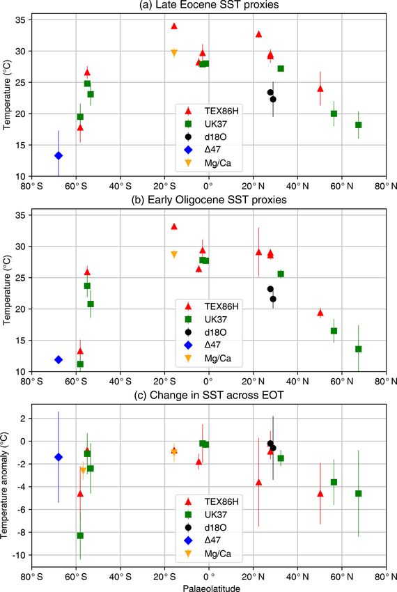
D. K. Hutchinson et al.: The Eocene–Oligocene transition                                                                      273

way below the level identified as “Oi-1” (Katz et al., 2008,       thic δ 18 O values of the Eocene and Oligocene. It is widely
p. 330). Hence it is not appropriate to use “EOT-2” to denote      suggested that it signifies the initiation of major sustained
the second step. Note, for clarity, the EOIS is not instanta-      Antarctic glaciation, most likely an early East Antarctic Ice
neous and several records show some “intermediate” values;         Sheet (EAIS) (Bohaty et al., 2012; Coxall et al., 2005; Ga-
its inferred duration in the records presented here is in the      leotti et al., 2016; Miller et al., 1987; Shackleton and Ken-
tens of thousands of years (40 kyr at Site 1218; Coxall et al.,    nett, 1975; Zachos et al., 1992). The EOGM is interpreted
2005).                                                             as an approximately 500 kyr long glacial maximum, with
   This brings us back to the definition of the “EOT”. Based       lower values visible in some records (Zachos et al., 1996;
on the stratigraphic record from Tanzania, Dunkley Jones et        Liu et al., 2004) (Fig. 1). Oxygen isotope maxima in the late
al. (2008) and Pearson et al. (2008) placed the base of the        Eocene imply substantial ephemeral precursor glaciations in
EOT at the extinction of the tropical warm-water nannofos-         the approach to the EOT (Galeotti et al., 2016; Houben et al.,
sil Discoaster saipanensis, a reliable bioevent which they re-     2012; Katz et al., 2008; Scher et al., 2011, 2014). The oldest
garded as the first sign of biotic extinction associated with      and most prominent of these hypothesised transient glacial
the late Eocene cooling. This extinction event has long been       events occurred at ∼ 37.3 Ma (within magnetochron C17n)
used to mark the base of nannofossil Zone NP21 (Martini,           and is referred to as the Priabonian oxygen isotope maxi-
1971) and more recently Zone CNE21 (Agnini et al., 2014).          mum (PrOM) Event (Scher et al., 2014). The “late Eocene
On the timescale used by Dunkley Jones et al. (2008) it was        event” of Katz et al. (2008) at ∼ 34.15 Ma may be regarded
estimated to be 500 kyr before the top of the EOIS. How-           as the second, the third being δ 18 O Step 1 at ∼ 34 Ma (the
ever, a subsequent calibration from ODP Site 1218 (Blaj et         “precursor glaciation” of Scher et al., 2011). Nevertheless,
al., 2009) placed this event significantly earlier than previ-     differences between δ 18 O curves from different water depths
ously suggested, which is supported by recent work in Java         and ocean regions, combined with increasing detail in indi-
(Jones et al., 2019). In the record from Site 1218 the D. saipa-   vidual records afforded by high-resolution sampling, empha-
nensis extinction is coincident (within 80 kyr analytical er-      sise that the EOT cannot be adequately understood as a series
ror; Coxall et al., 2005) with the base of a significant δ 18 O    of discrete events because it is clearly imprinted by orbitally
increase – possibly a “failed” glaciation – that seems to be       paced variability throughout (Coxall et al., 2005).
visible in many of the records (including Tanzania) and has           A detailed discussion of the Hantkenina extinction and as-
been termed the “late Eocene event” by Katz et al. (2008).         sociated bioevents at the EOB was provided by Berggren
It seems desirable to include these biotic and climatic events     et al. (2018, p. 30–32). The highest stratigraphic occurrence
within the definition of the EOT rather than insist on an arbi-    of the planktonic foraminifera family Hantkeninidae denotes
trary 500 kyr duration. On the most commonly used current          the EOB in its type section (Nocchi et al., 1986). This is
timescale, “Geological Timescale 2012” (GTS2012; Grad-             thought to have involved simultaneous extinction of all five
stein et al., 2012), the critical levels are calibrated as fol-    morphospecies and two genera of late Eocene hantkeninids
lows: top of the EOIS at 33.65 Ma, base of chron C13n at           (Coxall and Pearson, 2007) (Fig. 1). Insofar as the principles
33.705 Ma, EOB at 33.9 Ma and extinction of D. saipanensis         of biostratigraphy require a particular species to denote a bio-
at 34.44 Ma. Hence the stratigraphic interval of the EOT ac-       zone boundary, the commonest species, Hantkenina alaba-
cording to our preferred definition is now given an estimated      mensis, is used to define the base of Zone O1 (Berggren et al.,
duration of 790 kyr (Fig. 1). This terminology and the alter-      2018; Berggren and Pearson, 2005; Wade et al., 2011). The
natives are summarised in Table 1 and illustrated below in         extinction of H. alabamensis can be considered the “primary
Fig. 1.                                                            marker” for worldwide correlation of the EOB. It occurs at
   Combined δ 18 O and trace element investigations (see           a slightly higher (later) level than another set of prominent
Sect. 3.2) have led to the suggestion that the δ 18 O increase     planktonic foraminifer extinctions, namely Turborotalia cer-
commonly referred to as Step 1 (Fig. 1) is mostly attributable     roazulensis and related species. DSDP Site 522 (South At-
to ocean cooling, with subordinate ice sheet growth, whereas       lantic), thus far, is one of the few deep-sea records to have
the more prominent δ 18 O increase at the end of the EOT (i.e.     both a detailed δ 18 O stratigraphy and planktonic foraminifera
the EOIS in our terminology) largely represents ice growth         assemblages that capture these evolutionary events. Here, the
with a little further cooling (Bohaty et al., 2012; Katz et        Hantkenina extinction horizon occurs approximately two-
al., 2008; Lear et al., 2008). Estimates of the combined to-       thirds of the way through the EOT (Fig. 1). It occurs at a simi-
tal sea-level fall across the EOT are of the order of 70 m         lar relative position in the hemipelagic EOT sequence in Tan-
(Miller et al., 2008; Wilson et al., 2013), and microfacies and    zania (Pearson et al., 2008), also in unpublished data from In-
palaeontological records from shelf environments (Houben           dian Ocean ODP Site 757 (Coxall et al., unpublished). This
et al., 2012) are consistent with this generalisation. A recent    finding implies that the extinction of the hantkeninids was
shallow marine sediment record also indicates the onset of         approximately synchronous, although its cause is currently
major glaciation at ∼ 33.7 Ma (Gallagher et al., 2020), in         unknown. Existing constraints on the hantkeninid extinction
agreement with deep-sea records. The EOIS is the sharpest          horizon remain rather coarse in terms of sampling resolution
feature in most records, culminating with the highest ben-         compared to many isotopic records, and the matter will ben-

https://doi.org/10.5194/cp-17-269-2021                                                           Clim. Past, 17, 269–315, 2021
274                                                                D. K. Hutchinson et al.: The Eocene–Oligocene transition

efit greatly from incoming high-resolution records from Site       ning of the Priabonian (late Eocene), possibly connected with
U1411, which boasts both excellent (glassy) preservation and       global cooling (e.g. Wade and Pearson, 2008; note that the
orbital level sampling.                                            base of the Priabonian has recently been defined in the Alano
   Dating and correlation of non-marine records, which usu-        section in Italy; Agnini et al., 2020). These data are excluded
ally lack δ 18 O stratigraphy, is more challenging, and there      by our definition from the EOT but may be part of the same
are far fewer well-dated records on land. Here a strict con-       general long-term pattern. In some stratigraphic records, es-
cept of the EOT is difficult to apply and relies on correla-       pecially terrestrial ones, it may not be easy to distinguish
tions using other stratigraphic approaches, including magne-       these longer-term events from the EOT.
tostratigraphy and palynomorph or mammal tooth biostratig-
raphy, which have been cross-calibrated in a few marine and        2     Proxy evidence for palaeogeography, ocean
marginal-marine sections (Abels et al., 2011; Dupont-Nivet               circulation and terrestrial ice evolution
et al., 2007, 2008; Hooker et al., 2004). Central Asian sec-
tions are the exception, where even the step features of the       Here we discuss proxy evidence for the global palaeogeogra-
EOT can be identified using magneto-, bio- and cyclostratig-       phy of the EOT (Sect. 2.1), including the state and evolution
raphy (Xiao et al., 2010). Moreover, combined δ 18 O and           of ocean gateways (Sect. 2.2), and proxy evidence for ocean
clumped isotope analyses on freshwater gastropod shells            circulation (Sect. 2.3) and Antarctic glaciation (Sect. 2.4).
from a terrestrial EOT section in the south of England have        We then briefly discuss the timing of the Northern Hemi-
permitted the first direct correlation of marine and non-          sphere glaciation (Sect. 2.5).
marine realms and identified coupling between cooling and
hydrological changes in the terrestrial realm (Sheldon et al.,
                                                                   2.1    Tectonic reconstruction
2016). This finding suggests a close timing and causal re-
lation between the earliest Oligocene glaciation and a ma-         The tectonic evolution of the southern continents, opening
jor Eurasian mammalian turnover event called the “Grande           a pathway for the Antarctic Circumpolar Current (ACC),
Coupure” (Hooker et al., 2004; Sheldon et al., 2016). Dur-         has long been linked with long-term Eocene cooling and
ing the Grand Coupure, many endemic European mammal                the EOT (Kennett et al., 1975). However, there remain ma-
species became extinct and were replaced by Asian immi-            jor challenges in reconstructing the palaeogeography at or
grant species. These changes have been attributed to a com-        around the EOT, requiring a series of methodological steps
bination of climate-driven extinction and species dispersal        (Baatsen et al., 2016; Kennett et al., 1975; Markwick, 2007,
due to the closing of Turgai Strait, which provided a greater      2019; Markwick and Valdes, 2004; Müller et al., 2008). The
connection between Europe and Asia (Akhmetiev and Beni-            first step is to use modern geography and relocate the con-
amovski, 2009; Costa et al., 2011; Hooker et al., 2004).           tinental and ocean plates according to a plate tectonic evo-
   In shallow-water carbonate successions, the EOB has tra-        lution model, used in software such as GPlates (Boyden et
ditionally been approximated by the prominent extinctions of       al., 2011). This software uses the interpretation of seafloor
a series of long-ranging larger benthic foraminifers (LBFs),       spreading and palaeomagnetic data to reconstruct relative
often called orthophragminids (corresponding to the families       plate motion (e.g. Scotese et al., 1988) and an absolute refer-
Discocylinidae and Asterocyclinidae; Adams et al., 1986).          ence frame to position the plates relative to the Earth’s man-
The general expectation was that these extinctions likely oc-      tle (e.g. Dupont-Nivet et al., 2008). Currently, there are two
curred at the time of maximum ice growth and sea-level re-         such absolute reference frames: one based on a global net-
gression – in our terminology the EOIS. However evidence           work of volcanic hot spots (Seton et al., 2012) and one based
from Tanzania (Cotton and Pearson, 2011) and Indonesia             on a palaeomagnetic reference frame (van Hinsbergen et al.,
(Cotton et al., 2014) suggest that the extinctions occurred        2015; Torsvik et al., 2012). Importantly, these two reference
within the EOT. In Tanzania the extinctions occur quite pre-       frames give virtually the same continental outlines, but the
cisely at the level of the EOB, hinting that the EOB itself may    orientation of the continents is shifted. This results in differ-
have had a global cause affecting different environments,          ences in continental positions between the reference frames
possibly independent of the events that caused the isotope         of up to 5–6◦ (Baatsen et al., 2016) around the EOT, creating
increases (Cotton and Pearson, 2011).                              an uncertainty in reconstructing palaeogeography, especially
   The definition of the EOT used here excludes the long-          in southern latitudes between 40 and 70◦ S, where important
term Eocene cooling trend. That trend began in the Ypre-           land and ocean geological archives exist. This latitudinal un-
sian (early Eocene) and continued through much of the Lute-        certainty also impacts the reconstruction of Antarctic glacia-
tian and Bartonian (middle Eocene, albeit interrupted by the       tion, since glacial dynamics are highly sensitive to latitude.
middle Eocene climatic optimum (MECO); Bohaty and Za-                 After the plate tectonic reconstruction has been applied,
chos 2003) and Priabonian (late Eocene; Cramwinckel et al.,        adjustments are needed to capture the age–depth evolution of
2018; Inglis et al., 2015; Liu et al., 2018; Śliwińska et al.,   the seafloor (Crosby et al., 2006) and seafloor sedimentation
2019; Zachos et al., 2001). In particular, prominent extinc-       rate (Müller et al., 2008). Adjusting land topography is more
tions in various marine groups occurred around the begin-          difficult and requires knowledge of palaeo-altimetry, includ-

Clim. Past, 17, 269–315, 2021                                                          https://doi.org/10.5194/cp-17-269-2021
D. K. Hutchinson et al.: The Eocene–Oligocene transition 275
ing processes such as plate collision processes, uplift, sub- ern Ocean gateways (Barker and Burrell, 1977; Kennett,
sidence and erosion. Several publicly available reconstruc- 1977). This mechanism suggests that the onset of the ACC
tions exist for the Eocene; Markwick (2007) reconstructed reorganised ocean currents from a configuration of subpolar
palaeotopography for the late Eocene (38 Ma), while Sewall gyres with strong meridional heat transport to predominantly
et al. (2000) and more recently (Zhang et al., 2011) and zonal flow, thereby causing thermal isolation of Antarctica
Herold et al. (2014) have generated palaeotopographies for (Barker and Thomas, 2004). The hypothesis is supported by
the early Eocene (∼ 55 to 50 Ma). These are based on the foraminiferal isotopic evidence from deep-sea drill cores in
hot spot reference frame. Baatsen et al. (2016) have recently the Southern Ocean, which indicate a shift from warm to cold
created a palaeogeographic reconstruction of the late Eocene currents (Exon et al., 2004). As such, there has been consid-
using the Palaeomagnetic reference frame. Such efforts to de- erable effort to reconstruct the tectonic history of the South-
velop realistic palaeogeography for each time slice represent ern Ocean gateways.
a major undertaking in blending geomorphic evidence with The Drake Passage opening has been dated to around
tectonic evolution and thus include many specific details that 50 Ma (Livermore et al., 2007) or even earlier (Markwick,
are beyond the scope of this review. 2007); however it was likely shallow and narrow at this time.
Recently, a stage-by-stage palaeogeographic reconstruc- The timing of the transition to a wide and deep gateway, po-
tion of the entire Phanerozoic has been made publicly avail- tentially capable of sustaining a vigorous ACC, occurred on
able in digital format (Scotese and Wright, 2018). This in- a timescale of tens of millions of years. Even with substantial
cludes snapshots of the Priabonian (35.9 Ma) and Rupelian widening of Drake Passage, several intervening ridges in the
(31 Ma). Another stage-by-stage reconstruction of Ceno- region are likely to have blocked the deep circumpolar flow
zoic palaeogeography evolution originates from Markwick (Eagles et al., 2005). These barriers may not have cleared un-
(2007); this reconstruction has been incorporated into a til the Miocene at around 22 Ma (Barker and Thomas, 2004;
modelling study of climate dependence on palaeogeogra- Dalziel et al., 2013). The evolution of the Tasman Gate-
phy (Farnsworth et al., 2019; Lunt et al., 2016), and palaeo- way is better constrained. Geophysical reconstructions of
geography changes across the EOT (Kennedy et al., 2015). continent–ocean boundaries (Williams et al., 2011) place the
However, the most recent versions of the (Markwick, 2007) opening of a deep (greater than ∼ 500 m) Tasman Gateway
palaeogeography reconstructions are proprietary and are thus at 33.5 ± 1.5 Ma (Scher et al., 2015; Stickley et al., 2004).
not included in this paper. Therefore, we present a sum- Marine microfossil records suggest the circumpolar flow was
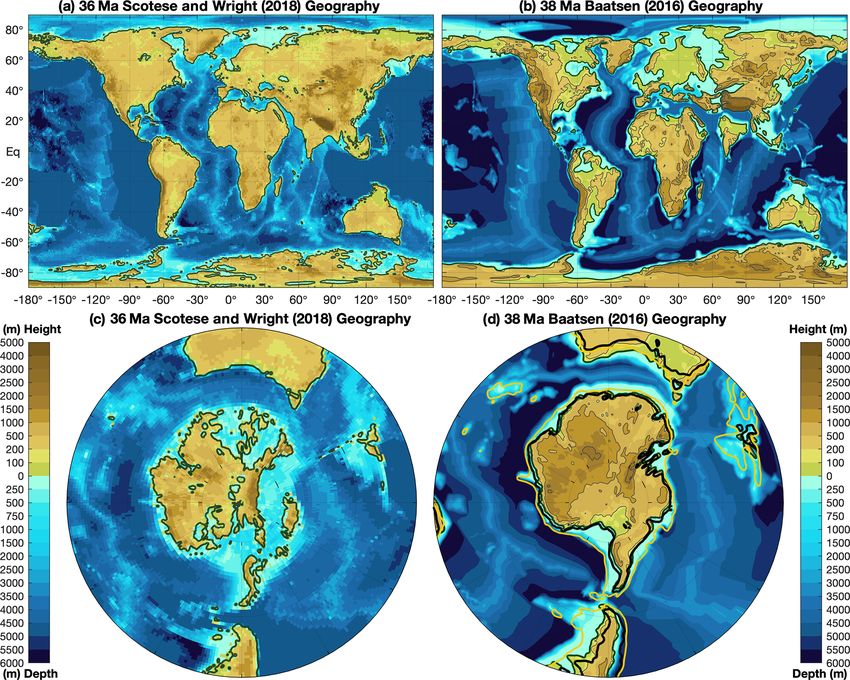
mary of late Eocene (38 Ma) palaeogeography in Fig. 2 from initially westward (Bijl et al., 2013). Multiproxy-based evi-
the publicly available datasets of Baatsen et al. (2016) and dence from ODP Leg 189 suggests that the opening of the
Scotese and Wright (2018). Our aim here is not to evaluate Tasman Gateway significantly preceded Antarctic glaciation
these reconstructions, but to present them such that their dif- and might therefore not have been its primary cause (Hu-
ferences can be taken as broadly indicative of the uncertain- ber et al., 2004; Stickley et al., 2004; Wei, 2004). The re-
ties in palaeogeography at this time. sults also indicate that the gateway deepening at the EOT ini-
The reconstructions contain several notable regions of un- tially produced an eastward flow of warm surface waters into
certainty which we briefly mention. They include (i) the Ti- the southwestern Pacific, not of cold surface waters as previ-
betan Plateau and the Indian subcontinent, where there are ously assumed. Subsequently, the Tasman Gateway steadily
clear disagreements between the reconstructions, (ii) the Tur- opened during the Oligocene, hypothesised to cross a thresh-
gai Strait and Tethys region, which has far greater shallow old when the northern margin of the ACC aligned with the
marine shelf regions in the Baatsen et al. (2016) reconstruc- westerly winds (Scher et al., 2015), triggering the onset of
tion, (iii) the Fram Strait, which is arguably closed by the an eastward-flowing ACC at around 30 Ma. However, the
Eocene–Oligocene transition but is open in both reconstruc- westerly winds can also shift position due to changes in oro-
tions (Lasabuda et al., 2018), and (iv) the Rocky Mountains graphic barriers or an increase in the meridional tempera-
and North American continent exhibit key differences in el- ture gradient after glaciation. Thus, the opening of Southern
evation and coastlines, which has implications for Eocene– Ocean gateways approximately coincides with the EOT, but
Oligocene climate evolution (Chamberlain et al., 2012). A with large uncertainty on the timing and implications. We
full review of these uncertainties is beyond the scope of this discuss modelling of this mechanism in Sect. 6.1.
paper, however we briefly discuss some impacts of these
palaeogeography uncertainties on terrestrial temperature re- 2.3 Meridional overturning circulation
constructions in Sect. 4, while we discuss the impacts on
ocean circulation in Sect. 2.2 and 2.3. Throughout much of the Eocene, deep-water formation is
suggested to have occurred dominantly in the Southern
2.2 Southern Ocean gateways
Ocean and the North Pacific (Ferreira et al., 2018), based
on numerical modelling and supported by stable and ra-
A long-held hypothesis on the cause of the EOT glaciation is diogenic isotope work (Cramer et al., 2009; McKinley et
that Antarctica cooled because of tectonic opening of South- al., 2019; Thomas et al., 2014). Compilations of δ 18 O and
https://doi.org/10.5194/cp-17-269-2021 Clim. Past, 17, 269–315, 2021
276                                                                     D. K. Hutchinson et al.: The Eocene–Oligocene transition

Figure 2. Palaeogeography in the late Eocene showing two alternative reconstructions. Panels (a) and (c) use the hot spot reference frame,
using the Scotese and Wright (2018) palaeogeography at 36 Ma, while panels (b) and (d) use the palaeomagnetic reference frame showing
the reconstruction of Baatsen et al. (2016) at 38 Ma. These two reconstructions use different methodologies and are presented as broadly
indicative of the uncertainties in palaeogeography at this time. Also shown in panel (d) are post-EOT coastlines at 30 Ma (black contours)
and 1000 m depth (orange contours), which illustrate the widening of the Southern Ocean gateways during the 8 Myr interval around the
EOT.

δ 13 C throughout the Atlantic Basin suggest that the Atlantic         Eocene are linked to obliquity forcing cycles (Vahlenkamp et
meridional overturning circulation (AMOC) either started up            al., 2018a, b). Moreover, interactions between the Arctic and
or strengthened at the EOT (Borrelli et al., 2014; Coxall et al.,      Atlantic oceans are gaining interest as potential triggers of
2018; Katz et al., 2011). This view of the AMOC expansion              a late Eocene proto-AMOC (Hutchinson et al., 2019). Data
is supported by a decrease in South Atlantic εNd around the            from the Labrador Sea and western North Atlantic margin
EOT (Via and Thomas, 2006). Significant seafloor spread-               indicate that North Atlantic waters became saltier and denser
ing was occurring in the Southern Hemisphere, such that                from 37 to 33 Ma (Coxall et al., 2018). This densification
these changes in ocean circulation have previously been ex-            may then have strengthened or even triggered an AMOC,
plained by the opening of Southern Ocean gateways (Borrelli            suggesting a possible forcing mechanism for Antarctic cool-
et al., 2014). However, studies of deep-sea sediment drifts            ing that predates the EOT and Southern Ocean gateway open-
suggest that some kind of North Atlantic overturning oper-             ings.
ated from the middle Eocene (Boyle et al., 2017; Hohbein                  Proxy records suggest that the Arctic Ocean was much
et al., 2012). This earlier onset is supported by climate mod-         fresher during the Eocene than the present day, with typical
elling that suggested that AMOC fluctuations in the middle             surface salinities around 20–25 psu and periodic excursions

Clim. Past, 17, 269–315, 2021                                                               https://doi.org/10.5194/cp-17-269-2021
D. K. Hutchinson et al.: The Eocene–Oligocene transition                                                                      277

to very low salinity conditions (< 10 psu) (Brinkhuis et al.,     modern proportions (Huang et al., 2014). This is consistent
2006; Kim et al., 2014; Waddell and Moore, 2008). Outflow         with approximations of ice volume based upon oxygen iso-
of this fresh surface water into the North Atlantic can po-       topes (Bohaty et al., 2012; Lear et al., 2008) and is supported
tentially prohibit deep-water formation (Baatsen et al., 2020;    by the record of relatively diverse vegetation around at least
Hutchinson et al., 2018). A new line of evidence suggests that    coastal regions of Antarctica through the Oligocene (Francis
deepening of the Greenland–Scotland Ridge around the EOT          et al., 2008).
may have enabled North Atlantic surface waters to become             Recent evidence has emerged of transient precursor
saltier (Abelson and Erez, 2017; Stärz et al., 2017), by allow-   Antarctic glaciations that occurred in the late Eocene (Carter
ing a deeper exchange between the basins. A related hypoth-       et al., 2017; Escutia et al., 2011; Passchier et al., 2017;
esis derived from sea-level and palaeo-shoreline estimates in     Scher et al., 2014), suggesting a “flickering” transition out
the Nordic seas is that the Arctic likely became isolated dur-    of the greenhouse. Importantly, several Southern Ocean sites
ing the Oligocene (Hegewald and Jokat, 2013; O’Regan et           revealed evidence that Antarctic glaciation induced crustal
al., 2011). Thus a gradual constriction of the connection be-     deformation and gravitational perturbations resulting in lo-
tween the Arctic and Atlantic presents a newly hypothesised       cal sea-level rise close to the young Antarctic Ice Sheet
priming mechanism for establishment of a well-developed           (Stocchi et al., 2013). Finally, detailed core sedimentary
AMOC (Coxall et al., 2018; Hutchinson et al., 2019).              records drilled close to Antarctica in the western Ross Sea
                                                                  invoke a transition from a modestly sized highly dynamic
2.4   Antarctic glaciation
                                                                  late Eocene–early Oligocene ice sheet, existing from ∼ 34–
                                                                  32.8 Ma, to a more stable continental-scale ice sheet there-
Although transient glacial events on Antarctica are proposed      after, which calved at the coastline (Galeotti et al., 2016).
for the late Eocene, the most significant long-term glacia-
tions likely began on East Antarctica in the Gamburtsev           2.5   Northern Hemisphere glaciation
Mountains and other highlands (Young et al., 2011) as a re-
sult of rapid global cooling in the early Oligocene around        While there is clear evidence for Antarctic glaciations at
33.7 Ma (EOGM, Fig. 1). Evidence for glacial discharge into       the EOT, the question of contemporaneous Northern Hemi-
open ocean basins in the earliest Oligocene is long estab-        sphere glaciation is contentious. The prevailing view is that
lished, with ice-rafted debris appearing in deep-sea South-       the Oligocene represented a non-modern-like state with only
ern Ocean sediment cores (Zachos et al., 1992). Since these       Antarctica glaciated (Westerhold et al., 2020; Zachos et al.,
initial results, efforts have continued to document and un-       2001). Glaciation in mountain areas around the globe is sug-
derstand early Cenozoic Antarctic ice dynamics (Barker et         gested to have followed through the Miocene and Pliocene,
al., 2007; Francis et al., 2008; McKay et al., 2016). Combin-     with evidence for the first significant build-up of ice on
ing perspectives from marine geology, geophysics, geochem-        Greenland (in the southern highlands) traced to the late
ical proxies and modelling, these efforts have largely focused    Miocene, sometime between 7.5 and 6 Ma (Bierman et al.,
on the evolution and stability of the early Oligocene Antarc-     2016; Larsen et al., 1994; Maslin et al., 1998; Pérez et al.,
tic ice sheets and estimates of ice volume contributions to       2018) or as early as 11 Ma (Helland and Holmes, 1997).
sea-level change. Other important developments in the study       Northern Hemisphere glaciation intensified during the late
of Antarctic ice include modelled thresholds for Antarctic        Pliocene (∼ 2.7 Ma), when large terrestrial glaciers began
glaciation (DeConto et al., 2008; Gasson et al., 2014) and        rhythmically advancing and retreating across North America,
improved reconstructions of Eocene–Oligocene subglacial           Greenland and Eurasia (Bailey et al., 2013; Ehlers and Gib-
bedrock topography (from airborne radar surveys). These           bard, 2007; Lunt et al., 2008; Maslin et al., 1998; Raymo,
bedrock reconstructions are important for reconstructing the      1994; De Schepper et al., 2014; Shackleton et al., 1984). It is
nucleation centres of precursor ice sheets (Scher et al., 2011,   important to note that a delay in Northern Hemisphere glacia-
2014) and subsequent development of continent-sized ice           tion relative to Antarctica is predicted by climate models –
sheets (Bo et al., 2009; Thomson et al., 2013; Wilson et al.,     the stabilising effect of the hysteresis in the height–mass bal-
2013; Wilson and Luyendyk, 2009; Young et al., 2011).             ance feedback becomes weaker with greater distance from
   Evidence for glaciation in the Weddell Sea and Ross Sea        the poles (Pollard and DeConto, 2005), because with de-
suggest that there was an increase in physical weathering         creasing latitude summers become warmer for a given radia-
over West Antarctica around the EOT (Anderson et al., 2011;       tive forcing (DeConto et al., 2008).
Ehrmann and Mackensen, 1992; Huang et al., 2014; Olivetti            Nevertheless, a series of studies (Tripati et al., 2005, 2008;
et al., 2015; Scher et al., 2011; Sorlien et al., 2007). How-     Tripati and Darby, 2018) argue that bipolar glaciation was
ever, in the Ross Sea, evidence suggests that an expansion        triggered in the Eocene and/or Oligocene. This suggestion
over West Antarctica in Marie Byrd Land occurred after the        is based on two lines of evidence from the sedimentary
EOT (Olivetti et al., 2013), while in the Weddell Sea sed-        record: (i) estimates of global seawater δ 18 O values (Tripati
imentation rates were still lower than in recent times, sug-      et al., 2005) and (ii) identification of ice-transported sedi-
gesting the West Antarctic Ice Sheet was not expanded to          ment grains inferred to have originated from Greenland in

https://doi.org/10.5194/cp-17-269-2021                                                          Clim. Past, 17, 269–315, 2021
278 D. K. Hutchinson et al.: The Eocene–Oligocene transition
both interior Arctic Ocean and subarctic Atlantic sediment history of the Eurekan orogeny, taking into account crustal
cores associated with the EOT (Eldrett et al., 2007), or earlier shortening (Gurnis et al., 2018), indicates a period of signifi-
(middle Eocene) (St. John, 2008; Tripati and Darby, 2018; cant compression in northern Greenland and Ellesmere from
Tripati et al., 2008). Certainly, several lines of evidence pro- 55 to 35 Ma (Gion et al., 2017) that was probably associated
vide support for winter sea ice in the Arctic from the mid- with uplift (Piepjohn et al., 2016). These latest tectonic in-
dle Eocene (Darby, 2014; St. John, 2008; Stickley et al., sights are compatible with insights from apatite fission track
2009) and perennial sea ice from 13 Ma (Krylov et al., 2008). and helium data that support the onset of a rapid phase of
It is possible that small mountain glaciers on east Green- exhumation of the east Greenland margin around 30 ± 5 Ma
land, perhaps comparable to the modern Franz Josef and (Bernard et al., 2016; Japsen et al., 2015). Together, these
Fox glaciers of New Zealand (which extend from the South- approaches support a view of high mountains on Greenland
ern Alps through lush rain forest), reached sea level during and Ellesmere that began eroding in the late Eocene to early
cooler orbital phases of the Eocene, intensifying in the late Oligocene with a greater possibility of supporting glaciers.
Eocene and early Oligocene (Eldrett et al., 2007). Yet the
results of a recent detailed analysis of expanded EOT sec-
3 Marine observations
tions from the North Atlantic’s modern-day “Iceberg Alley”
on the Newfoundland margin are inconsistent with the pres- 3.1 Sea surface temperature observations
ence of extensive ice sheets on southern and western Green-
land and the northeastern Canadian Arctic, contradicting the A key requirement for understanding the cause and conse-
suggestion of extensive early Northern Hemisphere glacia- quences of the Eocene–Oligocene climatic transition is good
tion in favour of a unipolar icehouse climate state at the spatial and temporal constraints on global temperatures, and
EOT (Spray et al., 2019). Furthermore, it is unlikely that ice our most numerous and well-resolved records of this un-
growth on land in the Northern Hemisphere was sufficiently doubtedly come from the oceans. Quantitative reconstruction
extensive to impact global seawater δ 18 O budgets or sea level of sea surface and deep-ocean temperatures has been ongoing
at the EOT (Coxall et al., 2005; Lear et al., 2008; Mudelsee et for decades. This requires use of various geochemical prox-
al., 2014). Marine SSTs and floral records from the subarc- ies, both to provide independent support for absolute tem-
tic and Arctic imply sustained warm temperatures and ex- perature estimates and because different proxy options are
tensive lowland temperate vegetation well into the middle available for different ocean and sedimentary settings, and
Miocene (O’Regan et al., 2011), which are not readily rec- deep-sea versus surface ocean water masses. Each method
onciled with large continental ice sheets fringing Greenland has its own limitations and uncertainties, resulting in a cur-
and other Arctic landmasses then or before this time. rently patchy but steadily improving view of global change.
From a theoretical perspective, climate and ice sheet mod- Quantitative assemblage-based SST proxies akin to transfer
elling suggest that the CO2 threshold for Northern Hemi- functions are not available because there are no living plank-
sphere ice sheet inception is fundamentally lower than for ton relatives of those from the EOT. For a thorough review of
Antarctica (DeConto et al., 2008; Gasson et al., 2014), im- pre-Quaternary marine SST proxies, and their strengths and
plying that the climate must be cooler to glaciate Greenland weaknesses, see Hollis et al. (2019).
than Antarctica. This is also consistent with evidence that the While SST is more heterogeneous than the deep sea, re-
modern Greenland Ice Sheet is highly sensitive to climatic construction of it in the EOT is in some ways currently
warming and that Greenland may have been almost ice-free more achievable than bottom water temperatures because
for extended periods even in the Pleistocene (Schaefer et al., more proxies are available, although there are still multi-
2016). This asymmetry between the Northern and South- ple confounding factors to consider. Classical marine δ 18 O
ern hemispheres in susceptibility to glaciation has been at- palaeothermometry extracted from the calcium carbonate
tributed to (i) the lower latitudes of the continents encircling shells of fossil planktonic (surface-floating) foraminifera is
the Arctic Ocean relative to the Antarctic, together with dif- especially complicated because of the combining influences
ferent ocean and atmospheric circulation patterns (DeConto of (i) compromised fossil preservation under the shallow late
et al., 2008; Gasson et al., 2012), and (ii) the ice sheet carry- Eocene ocean calcite compensation depth, limiting the avail-
ing capacity of the continents; it has been argued that Green- ability of planktonic records, and (ii) increasing δ 18 O of sea-
land topography was low during the Palaeogene compared to water as a consequence of ice sheet expansion, which en-
Antarctica, and extensive mountain building, providing high- riches ocean water and thus increases calcite δ 18 O – a signal
altitude terrain needed for glaciation, did not occur until the which can otherwise indicate cooling. However, a growing
late Miocene–Pliocene (Gasson et al., 2012; Japsen et al., number of clay-rich hemipelagic marine sequences contain-
2006; Solgaard et al., 2013). ing exceptionally well-preserved (glassy) fossil material are
But even on the question of Greenland topography there is yielding δ 18 O palaeotemperatures that provide useful SST
uncertainty. Reconstructions of plate kinematics in suspected perspectives. δ 18 O SSTs derived from glassy foraminifera
ice sheet nucleation sites (e.g. northern Greenland, Ellesmere (Haiblen et al., 2019; Norris and Wilson, 1998; Pearson et al.,
Island) are equivocal. Recent work on the plate kinematic 2001; Wilson et al., 2002; Wilson and Norris, 2001) contrast
Clim. Past, 17, 269–315, 2021 https://doi.org/10.5194/cp-17-269-2021D. K. Hutchinson et al.: The Eocene–Oligocene transition 279
0
K index is well established, the TEX
greatly from those measured on recrystalised “frosty” mate- While the U37 86 in-
rial (Sexton et al., 2006). A detailed compilation of glassy dex is relatively new and its accuracy as a palaeotemperature
versus recrystalised foraminiferal δ 18 O proxies around the proxy is under critical review. There have been several dif-
EOT is given in Piga (2020). ferent TEX86 indices developed, with different SST calibra-
Planktonic foraminifera Mg / Ca palaeothermometry pro- tions (e.g. TEX086 by Sluijs et al., 2009; TEXH 86 and TEX86
L
vides another means of quantifying SSTs (Evans et al., 2016; by Kim et al., 2010; Bayspar by Tierney and Tingley, 2015).
Lear et al., 2008); however such records are even more sparse As suggested by some of the recent studies conducted on cul-
than δ 18 O equivalents due to the scarcity of appropriate EOT tures of Thaumarchaeota, GDGT composition may be sensi-
fossils. This method is especially useful since, in theory, un- tive not only to SST but also to other factors such as oxygen
like δ 18 O it should be independent of Antarctic glaciation (O2 ) concentration (Qin et al., 2015) or ammonia oxidation
and, when coupled with δ 18 O palaeothermometry, past vari- rate (Hurley et al., 2016). Furthermore, there is uncertainty
ations in the δ 18 O composition of seawater, and thus ice vol- in the source of the GDGTs used for SST estimations, i.e.
ume changes may also be estimated (Lear et al., 2004, 2008; their production level in the water column and possible sum-
Mudelsee et al., 2014). The two key existing records are from mer biases, and therefore their value as an SST proxy. Recent
Tanzania (Lear et al., 2008) and the Gulf of Mexico (Evans reviews are available for both the palaeotemperatures U37 K0
et al., 2016; Wade et al., 2012). The Tanzanian planktonic (Brassell, 2014) and TEX86 (Hurley et al., 2016; Pearson and
Mg / Ca record provides cornerstone evidence for a perma- Ingalls, 2013; Qin et al., 2015; Tierney and Tingley, 2015).
nent 2.5 ◦ C tropical surface and bottom water cooling, and Despite these issues, in some studies where both U37 K 0 and
therefore likely global cooling, associated with the Step 1 TEX86 indices were applied, temperature estimations show
of the EOT (Fig. 1). The Gulf of Mexico Mg / Ca tempera- remarkably similar results (Liu et al., 2009), suggesting that
ture record resembles the biomarker-derived (i.e. TEX86 ; see TEX86 , after an evaluation of the source and the distribution
below) SST record from this site (Wade et al., 2012). Both of GDGTs (Inglis et al., 2015), can successfully be applied
imply a distinct and slightly larger surface cooling of 3–4 ◦ C as a palaeotemperature proxy. TEX86 is especially useful at
limited to Step 1. To what extent secular change in seawa- K 0 index saturates at about 29 ◦ C
lower latitudes, since the U37
ter Mg / Ca reconstruction might have influenced these ac- (Müller et al., 1998).
tual numbers is an ongoing question (Evans et al., 2018). Cross-latitude biomarker proxy records (U37 K 0 and TEX )
86
Clumped isotope palaeothermometry (Ghosh et al., 2006; suggest that SSTs were higher than today in both the late
Zaarur et al., 2013), also independent of seawater δ 18 O, is Eocene and early Oligocene SSTs, with annual means of up
still in its infancy, but this is a third method applicable to to 20 ◦ C at both 60◦ N and 60◦ S respectively and low merid-
calcareous microfossils that will help address some of these ional temperature gradients (Hollis et al., 2009; Liu et al.,
problems. Thus far only one clumped isotope (147 ) record 2009; Wade et al., 2012). One record from the Gulf of Mex-
from Maud Rise spans the EOT (Petersen and Schrag, 2015). ico (Wade et al., 2012) suggests consistently higher SSTs de-
This record shows cooling preceding the EOT, and then rela- rived from TEX86 than from inorganic proxies (Hollis et al.,
tively minor changes across the EOT. Early to middle Eocene 2009, 2012; Liu et al., 2009). Where records span the EOT
clumped isotope SST records are consistent with other prox- (i.e. ∼ 33–34 Ma), between 1 and 5 ◦ C of surface cooling in
ies, specifically cooler values at high southern latitudes com- both hemispheres is found. To date, temperature records from
pared to the early and middle Eocene (Evans et al., 2018). the high northern latitudes are sparse, but coverage from the
Many new SST records based on Mg / Ca and 147 are ex- high southern latitudes is richer, where several records sug-
pected in coming years. gest a cooling of subantarctic waters across the EOT of 4 to
In some regions, Eocene–Oligocene age sediments lack 8 ◦ C, although some records are indistinguishable from 0 ◦ C
biogenic calcium carbonates (e.g. Bijl et al., 2009). There- change (Fig. 3). In the low-latitude Pacific, Atlantic and In-
fore low- and non-calcareous areas, like the Arctic and high- dian Ocean tropical SSTs were significantly warmer than to-
latitudes of the North Atlantic and North Pacific, have suf- day in the late Eocene, with SSTs up to 31 ◦ C (Liu et al.,
fered for lack of palaeotemperature data. However, the de- 2009) or even ∼ 33 ◦ C (Lear et al., 2008; Wade et al., 2012).
velopment of independent organic proxies based on biomark- One TEX86 record from the Gulf of Mexico implies gradual
ers such as alkenones (U37 K 0 index; Brassell et al., 1986) and surface cooling of 3–4 ◦ C between ∼ 34 and 33 Ma (Wade et
glycerol dialkyl glycerol tetraethers (GDGTs) from the mem- al., 2012). TEX86 data from Site 803 in the tropical Pacific
brane lipids of Thaumarchaeota (TEX86 index; Schouten et show a large transient cooling of up to 6 ◦ C across the EOT;
al., 2002), which can be preserved in high-sedimentation set- however, such a large change in tropical temperatures is re-
tings close to continental margins or restricted basins where garded as unrealistic and is more likely caused by a reorgan-
carbonate is often scarce, has helped fill this gap. Impor- isation of the water column (Liu et al., 2009). We therefore
tantly, these organic biomarkers are often the only marine do not include Site 803 in our compilation of temperature
archive for palaeothermometry at high latitudes, where SST change across the EOT (Fig. 3).
constraints are particularly useful for model–data compar- Newly available records from the North Atlantic region are
isons. starting to challenge earlier evidence of homogeneous bipo-
https://doi.org/10.5194/cp-17-269-2021 Clim. Past, 17, 269–315, 2021You can also read