The Gaia-ESO survey: the non-universality of
←
→
Page content transcription
If your browser does not render page correctly, please read the page content below
Astronomy & Astrophysics manuscript no. 38055corr                                                                                     c ESO 2020
                                               June 11, 2020

                                                       The Gaia-ESO survey: the non-universality of the
                                                age–chemical-clocks–metallicity relations in the Galactic disc?,??
                                                 G. Casali1, 2 , L. Spina3, 18 , L. Magrini2 , A. Karakas3, 18 , C. Kobayashi4 , A. R. Casey3, 18 , S. Feltzing15 , M. Van der
                                                   Swaelmen2 , M. Tsantaki2 , P. Jofré11 , A. Bragaglia12 , D. Feuillet15 , T. Bensby15 , K. Biazzo16 , A. Gonneau5 , G.
                                                  Tautvaišienė17 , M. Baratella7 , V. Roccatagliata2, 8, 25 , E. Pancino2 , S. Sousa9 , V. Adibekyan9 , S. Martell19, 18 , A.
                                                  Bayo24 , R. J. Jackson23 , R. D. Jeffries23 , G. Gilmore5 , S. Randich2 , E. Alfaro14 , S. E. Koposov6 , A. J. Korn21 , A.
                                                Recio-Blanco22 , R. Smiljanic20 , E. Franciosini2 , A. Hourihane5 , L. Monaco10 , L. Morbidelli2 , G. Sacco2 , C. Worley5 ,
                                                                                                         S. Zaggia13
                                                                                                 (Affiliations can be found after the references)
arXiv:2006.05763v1 [astro-ph.GA] 10 Jun 2020

                                                                                                                  June 11, 2020

                                                                                                                  ABSTRACT

                                               Context. In the era of large spectroscopic surveys, massive databases of high-quality spectra coupled with the products of the Gaia satellite provide
                                               tools to outline a new picture of our Galaxy. In this framework, an important piece of information is provided by our ability to infer stellar ages,
                                               and consequently to sketch a Galactic timeline.
                                               Aims. We aim to provide empirical relations between stellar ages and abundance ratios for a sample of stars with very similar stellar parameters
                                               to those of the Sun, namely the so-called solar-like stars. We investigate the dependence on metallicity, and we apply our relations to independent
                                               samples, that is, the Gaia-ESO samples of open clusters and of field stars.
                                               Methods. We analyse high-resolution and high-signal-to-noise-ratio HARPS spectra of a sample of solar-like stars to obtain precise determinations
                                               of their atmospheric parameters and abundances for 25 elements and/or ions belonging to the main nucleosynthesis channels through differential
                                               spectral analysis, and of their ages through isochrone fitting.
                                               Results. We investigate the relations between stellar ages and several abundance ratios. For the abundance ratios with a steeper dependence on age,
                                               we perform multivariate linear regressions, in which we include the dependence on metallicity, [Fe/H]. We apply our best relations to a sample
                                               of open clusters located from the inner to the outer regions of the Galactic disc. Using our relations, we are able to recover the literature ages
                                               only for clusters located at RGC >7 kpc. The values that we obtain for the ages of the inner-disc clusters are much greater than the literature ones.
                                               In these clusters, the content of neutron capture elements, such as Y and Zr, is indeed lower than expected from chemical evolution models, and
                                               consequently their [Y/Mg] and [Y/Al] are lower than in clusters of the same age located in the solar neighbourhood. With our chemical evolution
                                               model and a set of empirical yields, we suggest that a strong dependence on the star formation history and metallicity-dependent stellar yields of
                                               s-process elements can substantially modify the slope of the [s/α]–[Fe/H]–age relation in different regions of the Galaxy.
                                               Conclusions. Our results point towards a non-universal relation [s/α]–[Fe/H]–age, indicating the existence of relations with different slopes and
                                               intercepts at different Galactocentric distances or for different star formation histories. Therefore, relations between ages and abundance ratios
                                               obtained from samples of stars located in a limited region of the Galaxy cannot be translated into general relations valid for the whole disc. A
                                               better understanding of the s-process at high metallicity is necessary to fully understand the origin of these variations.
                                               Key words. stars: abundances − Galaxy: abundances − Galaxy: disc − Galaxy: evolution − open clusters and associations: general

                                               1. Introduction                                                             ages for the different Galactic populations, which we can use to
                                                                                                                           sketch a Galactic timeline.
                                               Galactic astronomy is experiencing a golden age thanks to the
                                               data collected by the Gaia satellite (Bailer-Jones et al. 2018;                  Determination of stellar ages is usually based on isochrone
                                               Lindegren et al. 2018; Gaia Collaboration et al. 2018), com-                fitting: this technique fits a set of isochrones – lines of con-
                                               plemented by ground-based large spectroscopic surveys, such                 stant age derived from models – to a set of observed colour-
                                               as APOGEE (Majewski et al. 2017), Gaia-ESO (Gilmore et al.                  magnitude diagrams. However, during recent decades, several
                                               2012), GALAH (De Silva et al. 2015; Bland-Hawthorn et al.                   groups have investigated alternative methods to estimate stellar
                                               2018) and LAMOST (Deng et al. 2012; Cui et al. 2012). The                   ages, such as for instance the lithium-depletion boundary, as-
                                               combination of these data is providing a new multi-dimensional              teroseismology, gyrochronology, stellar activity (see Soderblom
                                               view of the structure of our Galaxy. In this framework, impor-              2010; Soderblom et al. 2014, for a review on the argument), and
                                               tant information is provided by our ability to determine stellar            chemical clocks (see, e.g. Masseron & Gilmore 2015; Feltzing
                                                                                                                           et al. 2017; Spina et al. 2018; Casali et al. 2019; Delgado Mena
                                                 ?                                                                         et al. 2019, among many papers). In particular, chemical clocks
                                                   Based on observations collected with the FLAMES instrument at
                                               VLT/UT2 telescope (Paranal Observatory, ESO, Chile), for the Gaia-          are abundance ratios that show a clear and possibly linear rela-
                                               ESO Large Public Spectroscopic Survey (188.B-3002, 193.B-0936).             tion with stellar age (in their linear or logarithmic form). The
                                               ??                                                                          idea is that these ratios, whose relation with stellar age has been
                                                   Tables 1, 2 and 3 are only available in electronic form at the CDS
                                               via anonymous ftp to cdsarc.u-strasbg.fr (130.79.128.5) or via              calibrated with targets of which the age has been accurately mea-
                                               http://cdsweb.u-strasbg.fr/cgi-bin/qcat?J/A+A/                              sured (e.g. star clusters, solar twins, asteroseismic targets), allow
                                                                                                                                                                      Article number, page 1 of 18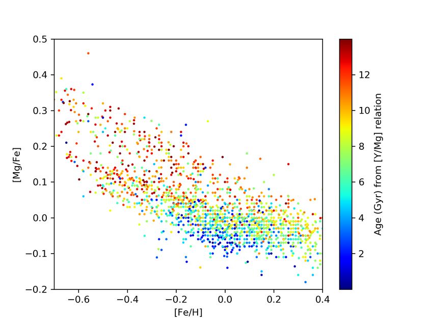
A&A proofs: manuscript no. 38055corr

us to derive the ages of large sample of stars through empirical       2. Spectral analysis
relations. Chemical clocks belong to two different broad fami-
lies: those based on the ratio between elements produced by dif-       2.1. Data sample and data reduction
ferent stellar progenitors, and thus with different timescales; and    In our analysis we employ stellar spectra collected by the
those based on the ratio between elements modified by stellar          HARPS spectrograph (Mayor et al. 2003). The instrument is in-
evolution, the alteration of which is strongly dependent on stel-      stalled on the 3.6 m telescope at the La Silla Observatory (Chile)
lar mass.                                                              and delivers a resolving power, R, of 115,000 over a 383 - 690
                                                                       nm wavelength range.
     The former, on which this work focuses, are based on pairs of         We obtain the reduced HARPS spectra from the ESO
elements produced with a different contribution of Type II (SNe        Archive. These are exposures of solar-like stars, with Teff within
II) and Type Ia (SNe Ia) supernovae or asymptotic giant branch         ±200 K and log g within ±0.2 dex from the solar parameters.
(AGB) stars. One of the first studies exploring the relation be-       In addition, for the analysis we select only spectra with signal-
tween chemical abundances and stellar age was da Silva et al.          to-noise ratios S/N>30 px−1 , which have been acquired with a
(2012). More recently, Nissen (2015) and Spina et al. (2016a)          mean seeing of 0.98”. This sample comprises 28,985 HARPS
found that ratios of [Y/Mg] and [Y/Al] are potentially good age        spectra of 560 stars. In Table 1, we list the dataset IDs, dates of
indicators in the case of solar twin stars (solar-like stars in the    observation, program IDs, seeing, exposure times, S/N and the
metallicity range of −0.1 to 0.1 dex); these were also used in         object names of the single spectra employed in the analysis.
other studies such as Nissen et al. (2017), Spina et al. (2018)            All spectra are normalised using IRAF1 ’s continuum and
and Delgado Mena et al. (2019). However, Feltzing et al. (2017)        are Doppler-shifted with dopcor using the stellar radial veloc-
and Delgado Mena et al. (2019) showed that when stars of dif-          ity value determined by the pipeline of the spectrograph. All the
ferent metallicities are included, these correlations might not be     exposures of a single object are stacked into a single spectrum
valid anywhere. There are also some studies on chemical clocks         using a Python script that computes the medians of the pixels af-
(e.g. [Y/Mg], [Ba/Mg]) in nearby dwarf galaxies, such as that by       ter having re-binned each spectrum to common wavelengths and
Skúladóttir et al. (2019).                                             applied a 3-σ clipping to the pixel values.
                                                                           In addition to the solar-like stars, the sample includes a solar
                                                                       spectrum acquired with the HARPS spectrograph through ob-
    High-resolution stellar spectra are necessary to determine ac-     servations of the asteroid Vesta to perform a differential analysis
curate stellar parameters and abundances, from which we can ob-        with respect to the Sun.
tain both stellar ages and abundance ratios. However, standard
spectroscopy can suffer from systematic errors, for instance in
the model atmospheres and modelling of stellar spectra (Asplund        2.2. Stellar parameters and chemical abundances
2005), because of the usual assumptions that affect stars with dif-
                                                                       Equivalent widths (EWs) of the atomic transitions of 25 elements
ferent stellar parameters and metallicity in different ways, such
                                                                       (i.e. C, Na, Mg, Al, Si, S, Ca, Sc, Ti, V, Cr, Mn, Fe, Co, Ni, Cu,
as for example static and homogeneous one-dimensional mod-
                                                                       Zn, Sr, Y, Zr, Ba, Ce, Nd, Sm, and Eu) reported in Meléndez et al.
els. To minimise the effects of systematic errors when studying
                                                                       (2014) and also employed in Spina et al. (2018) and Bedell et al.
solar-like stars, we can perform a differential analysis of those
                                                                       (2018) are measured with Stellar diff2 . We use the master
stars relative to the Sun (e.g. Meléndez et al. 2006; Meléndez
                                                                       list of atomic transitions of Meléndez et al. (2014) that includes
& Ramírez 2007). Their well-known stellar parameters are ex-
                                                                       98 lines of Fe I, 17 of Fe II, and 183 for the other elements,
tremely important for the calibration of fundamental observable
                                                                       detectable in the HARPS spectral range (3780-6910 Å).
quantities and stellar ages.
                                                                            This code allows the user to interactively select one or more
                                                                       spectral windows for the continuum setting around each line of
    Recent studies on solar twins have reached very high preci-        interest. Ideally, these windows coincide with regions devoid of
sion on stellar parameters and chemical abundances of the or-          other absorption lines. Once the continuum is set, we employ
der of 0.01 dex in Fe and 0.5 Gyr in age (e.g. Meléndez et al.         the same window settings to calculate continuum levels and fit
2009, 2014; Ramírez et al. 2009, 2014a,b; Liu et al. 2016; Spina       the lines of interest with Gaussian profiles in every stacked spec-
et al. 2016a,b, 2018), thanks to the differential analysis tech-       trum. Therefore, the same assumption is taken in the choice of
nique. This level of precision can be useful for revealing detailed    the local continuum around a single line of interest for all the
trends in the abundance ratios and opens the door to a more accu-      spectra analysed here. This is expected to minimise the effects
rate understanding of the Galactic chemical evolution, unveiling       of an imperfect spectral normalisation or unresolved features in
more details with respect to the large surveys.                        the continuum that can lead to larger errors in the differential
                                                                       abundances (Bedell et al. 2014). Furthermore, Stellar diff
                                                                       is able to identify points affected by hot pixels or cosmic rays
    The aim of the present paper is to study the [X/Fe] versus         and remove them from the calculation of the continuum. The
age relations. In Sect. 2, we present our data sets and describe       code delivers the EW of each line of interest along with its un-
our spectral analysis. In Sect. 3, we discuss the age–[X/Fe] rela-     certainty. The same method for the EW measurement was em-
tions. In Sect. 4, we present the relations between stellar ages and   ployed in the high-precision spectroscopic analysis of twin stars
chemical clocks. In Sect. 5, we investigate the non-universality       by Nagar et al. (2020).
of the relations involving s-process elements by comparing with
                                                                            We apply a line clipping, removing 19 lines of Fe I with un-
open clusters. In Sect. 6, we discuss the non-universality of the
                                                                       certainties on EWs lying out of the 95% of their probability dis-
relations between age and chemical abundances involving an s-
                                                                       tribution for more than five stars. These are removed for all of
process element. The application of the relations to the field stars
of Gaia-ESO high-resolution samples is analysed in Sect. 7. Fi-        1
                                                                         http://ast.noao.edu/data/software
nally, in Sect. 8, we summarise our results and give our conclu-       2
                                                                         Stellar diff is Python code publicly available at https://
sions.                                                                 github.com/andycasey/stellardiff.

Article number, page 2 of 18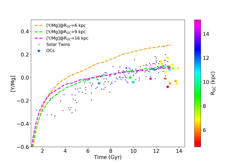
Casali, G. et al.: The non-universality of the age-[s-process/α]-[Fe/H] relations

Table 1. Information about the HARPS spectra of the sample of solar-like stars.

      Name                    Spectrum ID                        Observation date     Program ID        Seeing        Exposure Time (s)   S/N
      HD114853       HARPS.2017-03-12T04:22:10.194.fits            12/03/2017        198.C-0836(A)       0.70               900           271
      HD114853       HARPS.2017-07-11T23:49:19.456.fits            11/07/2017        198.C-0836(A)       1.32               900           285
      HD11505        HARPS.2011-09-27T06:37:22.718.fits            27/09/2011        183.C-0972(A)       0.96               900           279
      HD11505        HARPS.2011-09-16T07:05:21.491.fits            16/09/2011        183.C-0972(A)       0.89               900           219
      HD11505        HARPS.2007-10-14T04:10:42.910.fits            14/10/2007        072.C-0488(E)       0.93               900           281
      HD115231       HARPS.2005-05-12T02:34:31.050.fits            12/05/2005        075.C-0332(A)       0.49               900           193
      HD115231       HARPS.2005-05-13T02:40:27.841.fits            13/05/2005        075.C-0332(A)       0.99               900           171
      ...                           ...                                ...                 ...            ...                ...           ...

Notes. The full version of this table is available online at the CDS.

stars from the master line list to calculate their atmospheric pa-          the analysis presented here, the EWs are measured for these lines
rameters (Teff , log g, [Fe/H], ξ). The EW measurements are pro-            and MOOG is used to calculate the EWs taking the HFS into ac-
cessed by the qoyllur-quipu (q2) code3 (Ramírez et al. 2014b)               count (as described above). Although this is correct in principle,
which determines the stellar parameters through a line-by-line              it does leave the analysis open to some possible errors. Ideally,
differential analysis of the EWs of the iron lines relative to those        the lines should be fully modelled and the observed line shape
measured in the solar spectrum. Specifically, the q2 code itera-            compared with the modelled one (see e.g. Bensby et al. 2005;
tively searches for the three equilibria (excitation, ionisation, and       Feltzing et al. 2007). However, the analysis presented here is ro-
the trend between the iron abundances and the reduced equiva-               bust enough for our purposes, because we deal with stars that
lent width log[EW/λ]). The iterations are executed with a series            have very similar stellar parameters (Teff and log g close to so-
of steps starting from a set of initial parameters (i.e. the nom-           lar ones). This means that any systematic error should cancel to
inal solar parameters) and arriving at the final set of parame-             first order in the analysis. Finally, the q2 code determines the
ters that simultaneously fulfil the equilibria. We employ the Ku-           error budget associated with the abundances [X/H] by summing
rucz (ATLAS9) grid of model atmospheres (Castelli & Kurucz                  in quadrature the observational error due to the line-to-line scat-
2004), the version of MOOG 2014 (Sneden 1973), and we as-                   ter from the EW measurements (standard error), and the errors
sume the following solar parameters: Teff =5771 K, log g=4.44               in the atmospheric parameters. When only one line is detected,
dex, [Fe/H]=0.00 dex and ξ =1.00 km s−1 (Ayres et al. 2006).                as is the case for Sr and Eu, the observational error is estimated
The errors associated with the stellar parameters are evaluated             through the uncertainty on the EW measured by Stellar diff.
by the code following the procedure described in Epstein et al.             The final stellar parameters and chemical abundances are listed
(2010) and Bensby et al. (2014). Since each stellar parameter is            in Tables 2 and 3, respectively.
dependent on the others in the fulfilment of the three equilibrium
conditions, the propagation of the error also takes into account
this relation between the parameters. The typical precision for             2.3. Stellar ages
each parameter, which is the average of the distribution of the
errors, is σ(Teff )=10 K, σ(log g)=0.03 dex, σ([Fe/H])=0.01 dex,            During their lives, stars evolve along a well-defined stellar evo-
and σ(ξ) = 0.02 km s−1 .                                                    lutionary track in the Hertzsprung-Russell diagram that mainly
    This high precision is related to different factors: (i) the high       depends on their stellar mass and metallicity. Therefore, if the
S/N for a good continuum setting of each spectrum, with a typi-             stellar parameters are known with sufficient precision, it is pos-
cal value of 800 measured on the 65th spectral order (we calcu-             sible to estimate the age by comparing the observed properties
late the S/N for each combined spectrum as the sum in quadra-               with the corresponding model. Following this approach, we es-
ture of the subexposures); (ii) the high spectral resolution of             timate the stellar ages using the q2 code, which also computes a
HARPS spectrograph (R∼115,000) which allows blended lines                   probability distribution function for age for each star of our sam-
to be resolved; (iii) the differential line-by-line spectroscopic           ple. It makes use of a grid of isochrones to perform an isochrone
analysis, which allows us to subtract the dependence on log gf              fitting comparing the stellar parameters with the grid results and
and to reduce the systematic errors due to the atmospheric mod-             taking into account the uncertainties on the stellar parameters.
els, comparing stars very similar to the Sun; and (iv) the neg-             The q2 code uses the difference between the observed parame-
ligible contribution from telluric lines, since the spectra are the         ters and the corresponding values in the model grid as weight
median of several exposures, where the typical number is 50.                to calculate the probability distribution; it performs a maximum-
    Once the stellar parameters and the relative uncertainties              likelihood calculation to determine the most probable age (i.e.
are determined for each star, q2 employs the appropriate atmo-              the peak of the probability distribution). The q2 code also cal-
spheric model for the calculation of the chemical abundances.               culates the 68% and 95% confidence intervals, and the mean
All the elemental abundances are scaled relative to the values              and standard deviation of these values. We adopt the grid of
obtained for the Sun on a line-by-line basis. In addition, through          isochrones computed with the Yale-Potsdam Stellar Isochrones
the blends driver in the MOOG code and adopting the line list               (YaPSI) models (Spada et al. 2017). We take into account the
from the Kurucz database, q2 is able to take into account the hy-           α-enhancement effects on the model atmospheres, using the re-
perfine splitting effects in the abundance calculations of Y, Ba,           lation [M/H] = [Fe/H] + log(0.638 · 10[α/Fe] + 0.362) (Salaris
and Eu (we assumed the HFS line list adopted by Meléndez et al.             et al. 1993), where we employ magnesium as a proxy for the α-
2014). We note that lines for some elements suffer from HFS; in             abundances.
                                                                            Typical uncertainties on our age determinations (i.e. the average
3
  The q2 code is a free Python package, available online at https:          of the half widths of the 68% confidence intervals) are 0.9 Gyr.
//github.com/astroChasqui/q2.                                               The ages of the solar-like stars can be found in Table 2.
                                                                                                                         Article number, page 3 of 18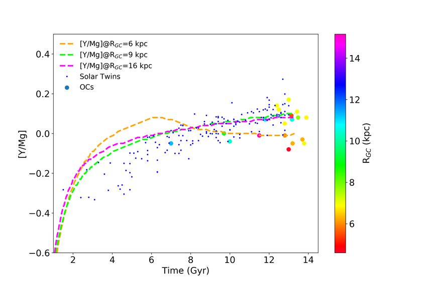
A&A proofs: manuscript no. 38055corr

Table 2. Atmospheric parameters and stellar ages determined for the sample of solar-like stars.

                id                 RA               DEC            Teff          logg           [Fe/H]             ξ           Age
                                 (J2000)                           (K)           (dex)           (dex)         (km s−1 )      (Gyr)
                HD220507       23:24:42.12     −52:42:06.76      5689±3       4.26±0.01      0.019±0.003      1.02±0.01     10.7±0.6
                HD207700       21:54:45.20     −73:26:18.55      5671±3       4.28±0.01      0.052±0.003      1.00±0.01     10.3±0.5
                HIP10303       02:12:46.64     −02:23:46.79      5710±3       4.39± 0.01     0.096±0.002      0.93±0.01      6.5±0.6
                HD115231       13:15:36.97     +09:00:57.71      5683±5       4.35±0.01      −0.098±0.003     0.97±0.01     10.7±0.6
                HIP65708       13:28:18.71     −00:50:24.70      5761±5       4.26±0.01      −0.047±0.004     1.12±0.01      9.9±0.5
                HD184768       19:36:00.65     +00:05:28.27      5687±4       4.31±0.01      −0.055±0.003     1.02±0.01     11.0±0.5
                HIP117367      23:47:52.41     +04:10:31.72      5866±3       4.36±0.01      0.024±0.003      1.14±0.01      5.6±0.5
                ...                 ...             ...             ...            ...             ...            ...           ...

Notes. The full version of this table is available online at the CDS.

Table 3. Chemical abundances for the sample of solar-like stars.

       id            [CI/H]       [NaI/H]        [MgI/H]         [AlI/H]         [SiI/H]         [SI/H]        [CaI/H]         [ScI/H]       [ScII/H]
   HD220507     0.145±0.021    0.062±0.007     0.161±0.015    0.175±0.007     0.085±0.002    0.084±0.015    0.070±0.004    0.092±0.023    0.126±0.011
   HD207700     0.171±0.012    0.094±0.008     0.169±0.014    0.208±0.010     0.115±0.003    0.120±0.006    0.099±0.004    0.129±0.027     0.157±0.01
   HIP10303      0.087±0.007   0.106±0.002     0.093±0.009    0.123±0.006     0.101±0.001    0.075±0.032    0.099±0.004    0.098±0.015    0.121±0.008
   HD115231     −0.038±0.011   −0.143±0.003    0.044±0.038     0.02±0.017     −0.047±0.003   −0.061±0.007   −0.019±0.005   −0.012±0.031   −0.011±0.006
   HIP65708      0.077±0.019   −0.026±0.021    0.053±0.007    0.074±0.003     0.003±0.003    −0.008±0.012   −0.003±0.006   0.013±0.017    0.043±0.013
   HD184768     0.098±0.155    −0.007±0.002    0.074±0.013     0.13±0.002     0.031±0.002    0.040±0.019    0.005±0.005    0.049±0.027    0.091±0.005
   HIP117367     0.003±0.082   0.076±0.012     0.040±0.006    0.052±0.005     0.047±0.002    0.031±0.013    0.021±0.004    0.033±0.007    0.056±0.006
        ...            ...           ...            ...             ...             ...            ...            ...             ...           ...
     [TiI/H]       [TiII/H]        [VI/H]         [CrI/H]        [CrII/H]       [MnI/H]         [FeI/H]        [FeII/H]        [CoI/H]        [NiI/H]
  0.124±0.005   0.127±0.006    0.089±0.006     0.032±0.006    0.025±0.009     −0.005±0.009   0.019±0.003    0.016 ±0.005   0.084±0.004    0.030±0.003
  0.160±0.005   0.148±0.007    0.137±0.007     0.070±0.006    0.057±0.010     0.066±0.006    0.052±0.003    0.050 ±0.005   0.145±0.003    0.076±0.003
  0.112±0.004   0.108±0.006    0.121±0.006     0.110±0.005    0.108±0.007     0.159±0.008    0.096±0.003    0.100 ±0.005   0.119±0.004    0.113±0.004
 0.025±0.006    0.003±0.007    −0.035±0.006    −0.087±0.006   −0.101±0.006    −0.207±0.010   −0.097±0.004   −0.101±0.007   −0.084±0.009   −0.123±0.004
 0.048±0.006    0.057±0.007    0.003±0.006     −0.051±0.006   −0.042±0.005    −0.140±0.007   −0.047±0.005   −0.047±0.006   −0.020±0.007   −0.058±0.004
 0.076±0.005    0.066±0.006    0.042±0.009     −0.050±0.005   −0.05±0.008     −0.101±0.009   −0.055±0.004   −0.055±0.006   0.043±0.004    −0.029±0.004
 0.030±0.005    0.039±0.005    0.029±0.005     0.020±0.004    0.031±0.007     0.013±0.006    0.025±0.003    0.021 ±0.005   0.042±0.007    0.035±0.003
        ...            ...           ...            ...             ...             ...            ...            ...             ...           ...
    [CuI/H]         [ZnI/H]       [SrI/H]         [YII/H]        [ZrII/H]       [BaII/H]       [CeII/H]       [NdII/H]        [SmII/H]       [EuII/H]
  0.103±0.036   0.138±0.022    −0.013±0.007    −0.036±0.01    −0.044±0.02     −0.028±0.005   0.041±0.017                    0.065±0.011   0.103±0.007
  0.145±0.034   0.180±0.024    0.001±0.006     −0.014±0.007   −0.038±0.023    0.002±0.008    0.074±0.016    0.064±0.010    0.065±0.008    0.126±0.007
  0.128±0.008   0.097±0.010    0.158±0.006     0.135±0.007    0.103±0.023     0.077±0.013    0.083±0.025    0.111±0.010                    0.081±0.008
 −0.116±0.010   −0.083±0.004   −0.097±0.007    −0.102±0.017   −0.066±0.008    −0.076±0.012   0.039±0.014    0.100±0.008    0.159±0.007     0.17±0.008
 −0.027±0.020   0.027±0.009    −0.101±0.008    −0.095±0.007   −0.091±0.009    −0.072±0.014   0.016±0.016    0.059±0.007    0.097±0.008    0.057±0.008
 0.024±0.025    0.081±0.022    −0.068±0.006    −0.114±0.007   −0.119±0.005    −0.107±0.005   −0.009±0.014                  0.004±0.012    0.041±0.008
 0.043±0.021    0.037±0.008    0.007±0.005     0.004±0.008    −0.015±0.005    −0.012±0.006   0.014±0.017    0.043±0.010    0.002±0.010    0.026±0.008
        ...            ...           ...            ...             ...             ...            ...           ...            ...             ...

Notes. The full version of this table is available online at the CDS.

2.4. A check on the spectroscopic log g                                       effect on the derived spectroscopic gravities. The median of the
                                                                              difference between the two log g is ∼0.02 dex, which is smaller
In Fig. 1, we present a comparison between the log g values de-               than the scatter due to their uncertainties of the order of ∼0.03
rived through our spectroscopic analysis and those from Gaia                  dex. Figure 1 shows that the consistency level of the two sets
photometry and parallaxes. Photometric gravities were obtained                of gravities depends on stellar metallicity. Namely, metal-rich
using the following equation                                                  stars have spectroscopic gravities that are slightly smaller than
log(g) = log(M/M ) + 0.4 × Mbol + 4 × log(Teff ) − 12.505               (1)   the photometric values, while those obtained for the metal-poor
                                                                              stars are higher. The slight discrepancy between the two gravi-
where M/M is the stellar mass (in solar mass units) com-                      ties could be imputed to a number of factors, including system-
puted through a maximum-likelihood calculation performed by                   atic effects in the differential analysis of stars with metallicities
q2 as described in the previous section, Mbol is the bolomet-                 that are different from that of the Sun, the dependence of the grid
ric magnitude obtained from the luminosity published in the                   of isochrones on stellar metallicity, or other assumptions on the
Gaia DR2 catalogue (Lindegren et al. 2018) using the relation                 photometric log g calculation.
Mbol = 4.75−2.5×log(L/L ), and Teff is the spectroscopic effec-
tive temperature (we tested the use of the Gaia photometric Teff
                                                                              2.5. Orbital parameters
and the variations in log g are negligible). In Fig. 1, we plot solar-
like stars with relative errors on their parallaxes lower than 10%            All stars in our sample are observed by the Gaia satellite, and
and with uncertainties on their stellar parameters within 90% of              they are available in the DR2 database. We use the GalPy4
their distributions. Photometric surface gravities derived via stel-          package of Python, in which the model MWpotential2014 for
lar distances agree fairly well with the spectroscopic gravities              the gravitational potential of the Milky Way is assumed (Bovy
suggesting that 3D non local thermodynamic equilibrium (non-
                                                                              4
LTE) effects on the FeI and FeII abundances have only a small                     Code available at http://github.com/jobovy/galpy

Article number, page 4 of 18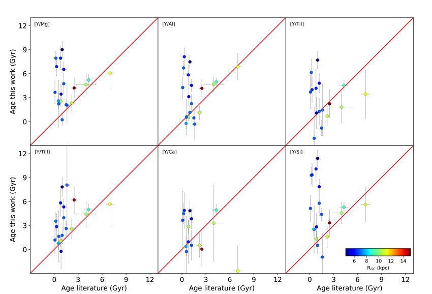
Casali, G. et al.: The non-universality of the age-[s-process/α]-[Fe/H] relations

Fig. 1. Comparison between photometric and spectroscopic log g,
where the stars are colour-coded by metallicity.

2015). Through AstroPy and the astrometric information by
Gaia DR2, we convert the celestial coordinates into the Galac-
tocentric radius (RGC ) and height above the Galactic plane (z),
assuming a solar Galactocentric distance R0 =8 kpc and a height
above the Plane z0 =0.025 kpc (Jurić et al. 2008). A circular ve-       Fig. 2. Distribution of the guiding radius Rg (top panel) and a distri-
locity at the solar Galactocentric distance equal to Vc = 220 km         bution of the eccentricity e (bottom panel) for our sample of solar-like
s−1 and the Sun’s motion with respect to the local standard of rest      stars.
[U ,V ,W ] = [11.1, 12.24, 7.25] km s−1 (Schönrich et al. 2010)
are used to calculate the Galactic space velocity (U,V,W) of each
star. As results of the orbit computation, we obtain, among sev-         colours: the red diamonds are thick-disc stars, whereas the
eral parameters, the eccentricity of the orbit e, the perigalacticon     thin-disc stars are shown with blue circles. We select the
and apogalacticon radii, and the guiding radius Rg .                     thick-disc stars through the [α/Fe] versus [Fe/H] plane with
    In Fig. 2 we present two different panels showing the distri-        [α/Fe]=([Ca/Fe]+[Si/Fe]+[Ti/Fe]+[Mg/Fe])/4 (excluding S be-
bution of guiding radius Rg and eccentricity e. Approximately            cause of its large scatter). The separation in chemical properties
95% of the stars in our sample have Rg between 6 and 9 kpc               is also related to the age separation between the two populations,
(top panel) and orbits with e < 0.3 (bottom panel). Only two             which is located at a look-back time of ∼8 Gyr (Haywood et al.
stars have a guiding radius of ∼4 - 4.5 kpc and very eccentric           2013; Nissen 2015; Bensby et al. 2014). The different slopes
orbits (e ∼ 0.6), implying their birth place is located far from the     for the relations of these elements versus age outline a differ-
solar neighbourhood. If we assume that the Rg is a good proxy            ent contribution of the main stellar nucleosynthesis processes,
of the Galactocentric distance where the stars were formed, then         such as for instance, those related to the ejecta of SNe II, SNe
we can conclude that the stars in our sample were born within            Ia, and AGB stars. As we can see from Fig. 3, the relations of
a restricted range of Galactocentric distances compared to the           [α/Fe] (with α elements of our sample Mg, Si, S, Ca, Ti) ver-
typical variation of the [X/Fe] ratios with Rg predicted by mod-         sus age have positive slopes, in agreement with their production
els (e.g. Magrini et al. 2009, 2017). However, it is possible that       over a shorter timescale with respect to iron. SNe II indeed eject
a fraction of the stars in our sample have not preserved their           mainly α-elements and elements up to the iron peak, including
kinematical properties due to interaction with spiral arms or gi-        Fe, into the interstellar medium (ISM) within short timescales
ant molecular clouds losing all information on their origin, and         (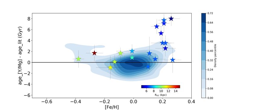
A&A proofs: manuscript no. 38055corr

Sr, Zr, Y) over iron have a negative slope due to their delayed       correlation coefficient for the chemical abundance ratios studied
production from successive captures of neutrons by iron-peak          in this work.
elements in low-mass AGB stars with respect to the early con-
tribution of SNe Ia and SNe II that produce iron. The elements
                                                                      4.2. Multivariate linear regression
with a lower contribution from the s-process and a high contri-
bution from the r-process, such as Eu (see Fig. 6 in Spina et al.     As shown in Fig. 4, the metallicity represents a third important
2018), have flatter [X/Fe]–age distributions than the almost pure     variable to take into account when we search for the relations
s-process elements. This means that the production of s-process       between abundance ratios and stellar age. Our sample, which is
elements has been more efficient within the last gigayear.            composed of stars similar to the Sun, is indeed a good way to
                                                                      test the metallicity dependence in a range from −0.7 to +0.4
                                                                      dex, disentangling the effect of the other parameters.
4. Chemical clocks                                                         In our analysis, we consider age (measured from the
                                                                      isochrone fitting via maximum-likelihood calculation) and
Abundance ratios of pairs of elements produced over different         metallicity (via spectroscopic analysis) as independent variables,
timescales (e.g. [Y/Mg] or [Y/Al) can be used as valuable indica-     while the abundance ratios are the dependent variables. We de-
tors of stellar age. Their [X/Fe] ratios show opposite behaviours     rive the relations in the form [A/B]= f (X), where X represents
with respect to stellar age (see e.g. [Mg/Fe] and [Y/Fe] in Fig. 3,   the independent variables, in this case age and [Fe/H], while
decreasing and increasing, respectively, with stellar age). There-    [A/B] is a generic abundance ratio used as a chemical clock.
fore, their ratio, for example [Y/Mg], shows a steep increas-         For each relation, we produce the adjusted R2 (adj-R2 ) param-
ing trend with stellar age. However, as pointed out by Feltz-         eter, a goodness-of-fit measurement for multivariate linear re-
ing et al. (2017) and Delgado Mena et al. (2019), their relations     gression models, taking into account the number of indepen-
might have a secondary dependence on metallicity. Moreover,           dent variables. We perform the fitting, selecting the best sam-
Titarenko et al. (2019) found the existence of different relations    ple of solar-like stars: ±100 K and ±0.1 dex from the Teff and
between ages and [Y/Mg] for a sample of stars belonging to the        the log g of the Sun, respectively. Stars with uncertainties on
thin and thick discs.                                                 stellar parameters and chemical abundances larger than 95% of
    The most studied chemical clocks in the literature are            their distributions or with uncertainties on age & 50% and stars
[Y/Mg] and [Y/Al] (Tucci Maia et al. 2016; Nissen 2015; Nis-          with an upper limit in age are excluded. These upper limits
sen et al. 2017; Slumstrup et al. 2017; Spina et al. 2016b, 2018).    are due to their probability age distributions, which are trun-
However, some recent studies have extended the list of chemi-         cated before they reach the maximum. This truncation due to
cal clocks to other ratios and found interesting results (Delgado     the border of the YAPSI isochrone grid excludes solar-like stars
Mena et al. 2019; Jofré et al. 2020).                                 younger than 1 Gyr. In addition, we identify and exclude stars
                                                                      that are anomalously rich in at least four s-elements in com-
4.1. Simple linear regression                                         parison to the bulk of thin disc stars. These are easily iden-
                                                                      tifiable because they lie outside 3-σ from a linear fit of data
In Fig. 4, we show the effect of metallicity in our sample            in Fig. 3: namely CWW097, HIP64150, HD140538, HD28701,
stars, where two chemical clocks ([Y/Mg] and [Y/Al]) are plot-        HD49983, HD6434, and HD89124. We also exclude a few stars
ted as a function of stellar age. The points are colour-coded         belonging to the halo (vtot > 200 km s−1 ).
by metallicity and the linear fits in four different metallicity           The parameters of the multivariate linear regressions are
bins ([Fe/H]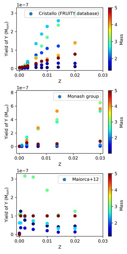
Casali, G. et al.: The non-universality of the age-[s-process/α]-[Fe/H] relations

Fig. 3. [X/Fe] ratio as a function of stellar age. The blue dots represent the thin disc stars, while the red diamonds are the thick disc populations.
The stars are within the metallicity range of −0.1 < [Fe/H] < +0.1 dex.

Fig. 4. [Y/Mg] and [Y/Al] as a function of age. The dots are colour-coded by [Fe/H]. The lines correspond to the linear functions described in
Table 4 in four different bins of metallicity: [Fe/H]
A&A proofs: manuscript no. 38055corr

Table 4. Slopes and intercepts of the four linear fits shown in Fig. 4.

                           [A/B]          metallicity bin            slope           intercept    Pearson coefficient
                           [Y/Mg]         [Fe/H] < −0.3          −0.038 ± 0.005   0.146 ± 0.050         −0.76
                           [Y/Mg]      −0.3 < [Fe/H] < −0.1      −0.042 ± 0.004   0.223 ± 0.029         −0.63
                           [Y/Mg]      −0.1 < [Fe/H] < +0.1      −0.040 ± 0.002   0.228 ± 0.015         −0.74
                           [Y/Mg]         [Fe/H] > +0.1          −0.018 ± 0.002   0.093 ± 0.010         −0.59
                           [Y/Al]         [Fe/H] < −0.3          −0.042 ± 0.005   0.212 ± 0.035         −0.83
                           [Y/Al]      −0.3 < [Fe/H] < −0.1      −0.048 ± 0.004   0.275 ± 0.031         −0.64
                           [Y/Al]      −0.1 < [Fe/H] < +0.1      −0.044 ± 0.002   0.241 ± 0.015         −0.79
                           [Y/Al]         [Fe/H] > +0.1          −0.025 ± 0.002   0.104 ± 0.012         −0.64

Fig. 5. Comparison of the ages derived by Delgado Mena et al. (2019) and those inferred in the present work with both of our relations: [Y/Mg]
and [Y/Al] vs. Age. The circles are the ages of the stars in common between the two works. The red lines are the one-to-one relations.

Table 5. Pearson coefficients of [A/B] abundance ratios vs. stellar age.   clusters available in the Gaia-ESO survey (GES) iDR5 with the
                                                                           corresponding ages derived using our stellar dating relations.
                    [A/B]       Pearson coefficient
                    [Y/Mg]            −0.87
                    [Y/Al]            −0.88                                5.1. The open cluster sample in the Gaia-ESO iDR5
                    [Y/Ca]            −0.87
                    [Y/Si]            −0.86                                We select open clusters (OCs) available in the Gaia-ESO iDR5
                    [Y/TiI]           −0.87                                survey (Gilmore et al. 2012; Randich et al. 2013, GES, here-
                    [Y/TiII]          −0.86                                after). We adopt the cluster membership analysis described in
                    [Y/Sc]            −0.84                                Casali et al. (2019). Briefly, the membership is based on a
                    [Y/V]             −0.84                                Bayesian approach, which takes into account both GES and Gaia
                    [Y/Co]            −0.80                                information. Membership probabilities are estimated from the
                    [Sr/Mg]           −0.84                                radial velocities (RVs; from GES) and proper motion velocities
                    [Sr/Al]           −0.87                                (from Gaia) of stars observed with the GIRAFFE spectrograph,
                    [Sr/TiI]          −0.83
                    [Sr/TiII]         −0.81
                                                                           using a maximum likelihood method (see Casali et al. 2019, for
                                                                           more details). For our analysis, we select stars with a minimum
                                                                           membership probability of 80%.
                                                                               The clusters are listed in Table 7, where we summarise their
                                                                           basic properties from the literature: coordinates, Galactocentric
                                                                           distances (RGC ), heights above the plane (z), median metallicity
this section, we compare the age from the literature for 19 open           [Fe/H], ages, and the references for ages and distances. We use
Article number, page 8 of 18
Casali, G. et al.: The non-universality of the age-[s-process/α]-[Fe/H] relations
Table 6. Multivariate linear regression parameters.
[A/B] c x1 x2 ∆c ∆x1 ∆x2 adj−R2 c0 x01 x02
[Y/Mg] 0.161 0.155 −0.031 0.009 0.028 0.002 0.80 5.245 5.057 −32.546
[Y/Al] 0.172 0.028 −0.035 0.009 0.029 0.002 0.78 4.954 0.796 −28.877
[Y/TiII] 0.132 0.146 −0.026 0.008 0.026 0.002 0.78 5.026 5.591 −38.219
[Y/TiI] 0.116 0.185 −0.025 0.008 0.024 0.001 0.81 4.597 7.326 −39.514
[Y/Ca] 0.099 0.142 −0.020 0.007 0.020 0.001 0.79 5.000 7.143 −50.462
[Y/Sc] 0.137 0.052 −0.026 0.009 0.029 0.002 0.67 5.304 2.017 −38.649
[Y/Si] 0.135 0.076 −0.025 0.008 0.025 0.001 0.75 5.311 3.003 −39.325
[Y/V] 0.116 −0.020 −0.024 0.008 0.026 0.002 0.66 4.869 −0.852 −41.921
[Y/Co] 0.163 −0.061 −0.029 0.009 0.029 0.002 0.67 5.699 −2.146 −35.018
[Sr/Mg] 0.184 0.218 −0.030 0.010 0.032 0.002 0.77 6.129 7.276 −33.401
[Sr/Al] 0.194 0.089 −0.034 0.010 0.031 0.002 0.77 5.737 2.631 −29.532
[Sr/TiI] 0.139 0.248 −0.025 0.009 0.028 0.002 0.78 5.655 10.103 −40.753
[Sr/TiII] 0.154 0.209 −0.025 0.010 0.031 0.002 0.74 6.052 8.203 −39.268
[Y/Zn] 0.170 −0.075 −0.029 0.009 0.028 0.002 0.68 5.853 −2.595 −34.370
[Sr/Zn] 0.194 −0.006 −0.029 0.010 0.032 0.002 0.65 6.819 −0.220 −35.072
[Sr/Si] 0.159 0.139 −0.025 0.010 0.031 0.002 0.70 6.341 5.553 −39.994
[Zn/Fe] −0.065 0.061 0.012 0.006 0.019 0.001 0.42 5.481 −5.180 84.381
Notes. Coefficients c, x1 , and x2 of the relations [A/B] = c+x1 ·[Fe/H]+x2 ·Age, where [Fe/H] and age are the independent variables. ∆c, ∆x1 , and
∆x2 are the uncertainties on the coefficients. c0 , x01 , and x02 are the coefficients of the inverted stellar dating relation Age = c0 +x01 ·[Fe/H]+x02 ·[A/B].
Finally, adj−R2 is the adjusted R2 parameter.
homogeneous data sets for age from the GES papers mentioned derived from the age of stellar associations to which they belong
above. or they are calculated through gyrochronologic measurements:
HD1835 (600 Myr, in Hyades, Rosén et al. 2016), HIP42333,
HIP22263 (0.3±0.1 Gyr, 0.5±0.1 Gyr, Aguilera-Gómez et al.
5.2. Age re-determination with chemical clocks 2018), HIP19781 (in Hyades, Leão et al. 2019), HD209779 (55
To compare the two data sets, we compute the median abundance Myr, in IC2391, Montes et al. 2001). In Fig. 6 we show the lo-
ratios of giant and subgiant star members in each cluster. In ad- cation of the five young solar-like stars with our sample of solar-
dition, since the abundances in GES are in the 12 + log(X/H) like stars. These follow the same trend as the solar-like stars with
form, we need to define our abundance reference to obtain abun- ages > 1 Gyr, demonstrating the continuity between the two sam-
dances on the solar scale – in order to have the abundances in ples and allowing us to extrapolate our relations up to 0.05 Gyr,
the [X/H] scale to compare with the solar-like stars. Table 8 the age of the youngest solar-like star in the sample.
shows three different sets of abundances: the solar abundances In Fig. 7, we show the abundance ratios of the solar-like stars
from iDR5 computed from archive solar spectra, the solar abun- versus age, together with those of OCs in the metallicity bin of
dances by Grevesse et al. (2007), and the median abundances −0.4A&A proofs: manuscript no. 38055corr
Table 7. Parameters of the open clusters in the GES sample.
Cluster RA(a) DEC(a) RGC z [Fe/H](a) Age Ref. Age & Distance
(J2000) (kpc) (pc) (dex) (Gyr)
NGC 6067 16:13:11 −54:13:06 6.81±0.12 −55±17 0.2 ± 0.08 0.1 ± 0.05 Alonso-Santiago et al. (2017)
NGC 6259 17:00:45 −44:39:18 7.03±0.01 −27±13 0.21 ± 0.04 0.21 ± 0.03 Mermilliod et al. (2001)
NGC 6705 18:51:05 −06:16:12 6.33±0.16 −95±10 0.16 ± 0.04 0.3 ± 0.05 Cantat-Gaudin et al. (2014)
NGC 6633 18:27:15 +06 30 30 7.71 −0.01 ± 0.11 0.52 ± 0.1 Randich et al. (2018)
NGC 4815 12:57:59 −64:57:36 6.94±0.04 −95±6 0.11 ± 0.01 0.57 ± 0.07 Friel et al. (2014)
NGC 6005 15:55:48 −57:26:12 5.97±0.34 −140±30 0.19 ± 0.02 0.7 ± 0.05 Hatzidimitriou et al. (2019)
Trumpler 23 16:00:50 −53:31:23 6.25±0.15 −18±2 0.21 ± 0.04 0.8 ± 0.1 Jacobson et al. (2016a)
Melotte 71 07:37:30 −12:04:00 10.50±0.10 +210±20 −0.09 ± 0.03 0.83 ± 0.18 Salaris et al. (2004)
Berkeley 81 19:01:36 −00:31:00 5.49±0.10 −126±7 0.22 ± 0.07 0.86 ± 0.1 Magrini et al. (2015)
NGC 6802 19:30:35 +20:15:42 6.96±0.07 +36±3 0.1 ± 0.02 1.0 ± 0.1 Jacobson et al. (2016a)
Rup 134 17:52:43 −29:33:00 4.60±0.10 −100±10 0.26 ± 0.06 1.0 ± 0.2 Carraro et al. (2006)
Pismis 18 13:36:55 −62:05:36 6.85±0.17 +12±2 0.22 ± 0.04 1.2 ± 0.04 Piatti et al. (1998)
Trumpler 20 12:39:32 −60:37:36 6.86±0.01 +134±4 0.15 ± 0.07 1.5 ± 0.15 Donati et al. (2014)
Berkeley 44 19:17:12 +19:33:00 6.91±0.12 +130±20 0.27 ± 0.06 1.6 ± 0.3 Jacobson et al. (2016b)
NGC 2420 07:38:23 +21:34:24 10.76 −0.13 ± 0.04 2.2 ± 0.3 Salaris et al. (2004); Sharma et al. (2006)
Berkeley 31 06:57:36 +08:16:00 15.16±0.40 +340±30 −0.27 ± 0.06 2.5 ± 0.3 Cignoni et al. (2011a)
NGC 2243 06:29:34 −31:17:00 10.40±0.20 +1200±100 −0.38 ± 0.04 4.0 ± 1.2 Bragaglia & Tosi (2006)
M67 08:51:18 +11:48:00 9.05±0.20 +405±40 −0.01 ± 0.04 4.3 ± 0.5 Salaris et al. (2004)
Berkeley 36 07:16:06 −13:06:00 11.30±0.20 −40±10 −0.16 ± 0.1 7.0 ± 0.5 Cignoni et al. (2011b)
Notes. (a) Magrini et al. (2018a)
Fig. 6. Abundance ratio vs. stellar age. The blue dots are our sample of solar-like stars and the red diamonds represent the five solar-like stars with
ages from the literature and abundances from our analysis.
on the residuals both for solar-like stars (the density contour) solar metallicity regime (−0.1Casali, G. et al.: The non-universality of the age-[s-process/α]-[Fe/H] relations
Fig. 7. Abundance ratio vs. stellar age. The blue dots show the values of our solar-like stars and the red stars represent the mean values for the
open clusters in the GES sample.
Table 8. Abundance references. novae during the final stages of the evolution of massive stars on
shorter timescales. Combining the enrichment timescales of the
Element Sun (iDR5) Sun (Grevesse et al. 2007) M67 giants (iDR5) s-process and α-elements, younger stars are indeed expected to
MgI 7.51±0.07 7.53±0.09 7.51±0.02(±0.05) have higher [s/α] ratios than older stars. However, the level of
AlI 6.34±0.04 6.37±0.06 6.41±0.01(±0.04) [s/α] reached in different parts of the Galaxy at the same epoch
SiI 7.48±0.06 7.51±0.04 7.55±0.01(±0.06) is not expected to be the same. Enlarging the sample of stars or
CaI 6.31±0.12 6.31±0.04 6.44±0.01(±0.10) star clusters outside the solar neighbourhood means that we have
TiI 4.90±0.08 4.90±0.06 4.90±0.01(±0.09)
TiII 4.99±0.07 – 5.01±0.01(±0.10) to deal with the complexity of the Galactic chemical evolution.
YII 2.19±0.12 2.21±0.02 2.15±0.01(±0.09) This includes radial variation of the star formation history (SFH)
in the disc driven by an exponentially declining infall rate and a
decreasing star formation efficiency towards the outer regions
(see, e.g. Magrini et al. 2009, and in general, multi-zone chem-
6. The non-universality of the relations between ical evolution models). Consequently, different radial regions of
the disc experience different SFHs, which produce different dis-
ages and abundance ratios involving s-process tributions in age and metallicity of the stellar populations. At
elements each Galactocentric distance, the abundance of unevolved stars,
which inherited heavy nuclei from the contributions of previous
The aim of the present study, together with other previous works generations of stars, is thus affected by the past SFH. Last but
(e.g. Feltzing et al. 2017; Spina et al. 2018; Delgado Mena et al. not least, there is a strong metallicity dependence of the stellar
2019, among many others), is to find stellar dating relations be- yields. The metallicity dependence of the stellar yield is partic-
tween ages and some abundance ratios that are applicable to the ularly important for neutron-capture elements produced through
whole Galaxy, or at least to vast portions of it. The opening ques- the s-process. Indeed, being secondary elements, the production
tions in Feltzing et al. (2017) focus on the possible universality of the s-process elements strongly depends on the quantity of
of the correlation between for example [Y/Mg] and age found in seeds (iron) present in the star. However, at high metallicity the
a sample of the solar-like stars, and, if it holds, also for larger number of iron seeds is much larger than the number of neu-
ranges of [Fe/H], or for stars much further than the solar neigh- trons. Consequently, in the super-solar metallicity regime, a less
bourhood or in different Galactic populations, such as those in effective production of neutron-capture elements with respect to
the thick disc. iron is predicted (Busso et al. 2001; Karakas & Lugaro 2016).
As we mention in Sect. 3, s-processes occur in low- and In addition, at high metallicity there might be a lower number of
intermediate-mass AGB stars (see, e.g. Busso et al. 2001; thermal pulses during the AGB phase, with a consequent lower
Karakas & Lugaro 2016), with timescales ranging from less final yield of s-process elements (see, e.g. Goriely & Siess 2018).
than a gigayear to several gigayears for the higher and lower Moreover, the production of Mg also depends on metallicity, in
mass AGB stars, respectively. On the other hand, α elements particular at high [Fe/H] where stellar rotation during the lat-
(in different percentages) are produced by core-collapse super-
Article number, page 11 of 18A&A proofs: manuscript no. 38055corr
Table 9. Abundance ratios of open clusters in the GES sample.
Cluster # stars [Y/Mg] [Y/Al] [Y/TiI] [Y/TiII] [Y/Ca] [Y/Si]
(dex) (dex) (dex) (dex) (dex) (dex)
Berkeley 31 5 (G) −0.01±0.03 0.02±0.03 0.01±0.04 −0.07±0.04 0.06±0.04 0.03±0.04
Berkeley 36 5 (G) −0.05±0.06 −0.07±0.06 0.00±0.07 −0.04±0.07 0.13±0.06 −0.02±0.06
Berkeley 44 7 (G) 0.14±0.07 0.19±0.07 0.13±0.08 −0.04±0.14 0.26±0.07 0.18±0.07
Berkeley 81 13 (G) 0.09±0.03 0.07±0.03 0.13±0.05 0.17±0.05 0.19±0.04 0.08±0.04
M67 3 (G) 0.00±0.01 0.00±0.01 0.00±0.01 0.00±0.01 0.00±0.01 0.00±0.01
Melotte 71 4 (G) 0.07±0.01 0.15±0.01 0.13±0.02 0.09±0.01 0.03±0.01 0.09±0.03
NGC 2243 17 (G, 1 SG) −0.04±0.03 0.00±0.03 0.00±0.05 −0.04±0.04 −0.02±0.09 −0.01±0.03
NGC 2420 28 (24 G, 4 SG) 0.07±0.03 0.13±0.03 0.08±0.03 0.04±0.03 0.07±0.03 0.08±0.03
NGC 4815 6 (G) 0.11±0.09 0.16±0.08 0.19±0.10 0.10±0.08 0.12±0.09 0.08±0.07
NGC 6005 9 (G) −0.01±0.02 0.02±0.02 0.03±0.03 0.02±0.02 0.05±0.02 −0.05±0.02
NGC 6067 12 (G) 0.08±0.04 0.03±0.05 0.06±0.05 0.13±0.04 0.05±0.07 0.02±0.04
NGC 6259 12 (G) −0.05±0.02 −0.05±0.02 0.00±0.04 0.07±0.03 0.04±0.02 −0.08±0.02
NGC 6633 3 (G) 0.08±0.02 0.18±0.02 0.19±0.02 0.11±0.01 0.09±0.01 0.07±0.01
NGC 6705 28 (G) −0.03±0.03 −0.10±0.03 0.05±0.04 0.08±0.04 0.02±0.04 −0.09±0.03
NGC 6802 10 (G) 0.17±0.02 0.14±0.02 0.23±0.03 0.10±0.02 0.24±0.02 0.13±0.02
Rup 134 16 (G) −0.08±0.02 −0.08±0.02 −0.03±0.02 −0.04±0.02 0.04±0.02 −0.14±0.02
Pismis 18 6 (G) 0.05±0.04 0.10±0.04 0.13±0.04 0.06±0.04 0.12±0.04 0.00±0.04
Trumpler 20 33 (31 G, 1 SG) 0.12±0.02 0.16±0.02 0.17±0.02 0.08±0.02 0.15±0.02 0.04±0.02
Trumpler 23 10 (G) −0.05±0.04 −0.02±0.04 0.05±0.06 0.01±0.04 0.11±0.05 −0.10±0.04
Notes. G: giants, SG: sub-giants.
Fig. 8. Comparison between the ages from the literature and the ages inferred in the present work for the open clusters. The symbols are colour-
coded by their Galactocentric distances. We note that we only show positive upper limit ages in this plot.
est phases of the evolution of massive stars increases the yield chemical clocks for a sample of the solar-like stars in the solar
of Mg (Romano et al. 2010; Magrini et al. 2017). The interplay neighbourhood, considering a large metallicity range to investi-
between the stellar yield and the metallicity of progenitors pro- gate their metallicity dependence. This was discussed in Sect. 4.
duces a different evolution at different Galactocentric distances.
Here, we present the analysis of stars located far away from
The combination of these dependencies points toward a re- the solar neighbourhood using a sample of open clusters ob-
lation between [Y/Mg], or in general [s/α], and age that changes served by the Gaia-ESO with a precise determination of age
with Galactocentric distance. Following the suggestions of Feltz- and distance. The sample gives us important indications on
ing et al. (2017), we first study the stellar dating relations from the variation of the [s/α] in different parts of the Galaxy. In
Article number, page 12 of 18Casali, G. et al.: The non-universality of the age-[s-process/α]-[Fe/H] relations
and solar-like stars very well. The agreement is completely lost
at RGC =6 kpc, where the faster enrichment of the inner disc for
GCE produces a higher [Y/Mg], which is not observed in the
open clusters. Similar results are obtained adopting the yields
from the FRUITY database (Domínguez et al. 2011; Cristallo
et al. 2011), and from the Monash group (Lugaro et al. 2012;
Fishlock et al. 2014; Karakas et al. 2014; Shingles et al. 2015;
Karakas & Lugaro 2016; Karakas et al. 2018) in the GCE. As
shown in Fig. 12, in which the yields of yttrium Y are shown in
different bins of metallicity Z for different stellar masses (1.3,
1.5, 2, 2.5, 3, 4, 5 M ), we can see that in the first two sets
of yields the production of s-process elements increases at high
metallicity. This produces an increasing abundance of s-process
elements in the inner disc, which is not observed in the abun-
Fig. 9. Residuals between the chemical-clock ages from [Y/Mg] and dances of the open cluster sample. The yields by Maiorca et al.
the literature ages as a function of [Fe/H]. The contours represent the (2012) have a flatter trend with the metallicity, which is not able
density of the sample of solar-like stars, while the stars represent the to reproduce the behavior of open clusters with RGC 9 kpc. Moreover, along the OC data, 6.2. A suggestion for the need for new s-process yields at
we also plot the Gaia-ESO samples of inner disc stars (labeled high metallicity
with GE_MW_BL in the GES survey) and those from the so- We investigate which set of empirical yields is necessary to
lar neighbourhood (GE_MW). We calculate their Galactocentric reproduce the observed lower trends, i.e. [Y/Mg] or [Y/Al]
distances from coordinates RA, DEC, and parallaxes of Gaia versus age, in the inner disc than in the solar neighbourhood.
DR2 as explained in Sect. 2.5. Field stars show a behaviour that The s-process element yields depend on the metallicity in two
is similar to that of the OCs, with a lower [Y/Mg] for the inner different ways; that is, they depend (i) on the number of iron
Milky Way populations (i.e. for RGC < 8 kpc). It is interesting to nuclei as seeds for the neutron captures, and (ii) on the flux
notice that in the inner disc, the bulk of field stars, usually older of neutrons. The former decreases with decreasing metallicity,
than stars in clusters, show an even lower [s/α] than the open while the latter increases because the main neutron source –
cluster stars. 13
C – is a primary process. 13 C is produced by mixing protons
into the He-shell present in low-mass AGB stars, where they are
6.1. The overproduction of s-process elements at high [Fe/H] captured by the abundant 12 C, which itself is produced during
the 3α process (also a primary process). This means that the
As shown in the previous sections, stars with the same age but amount of 13 C does not depend on the metallicity. The neutron
located in different regions of the Galaxy have different compo- flux depends (approximately) on 13 C/56 Fe, which increases with
sition. Thus, the stellar dating relations between abundance ra- decreasing metallicity. This means there are more neutrons per
tios and stellar ages based on a sample of stars located in limited seed in low-metallicity AGB stars and less in high-metallicity
volumes of the Galaxy cannot be easily translated into general AGB stars (see Busso et al. 2001; Karakas & Lugaro 2016).
stellar dating relations valid for the whole disc. Consequently, we should expect less s-process elements to be
The driving reason for this is that the SFH strongly effects produced at high metallicity.
the abundances of the s-process elements and the yields of low-
and intermediate-mass stars depend non-monotonically on the We tested a set of yields to investigate their behaviour at high
metallicity (Feltzing et al. 2017). This effect was already noticed metallicity. Yields for subsolar metallicities were left unchanged
by Magrini et al. (2018a, see their Fig 11), where [Y/Ba] ver- from their Maiorca et al. (2012) values, while we depressed the
sus age was plotted in different bins of metallicity and Galac- yields at super-solar metallicity by a factor of ten. In Fig. 13, we
tocentric distance. The innermost bin, dominated by metal rich show the time evolution of [Y/Mg] in three radial regions of our
stars, shows a different behaviour with respect to the bins located Galaxy adopting our empirical yields for Y. The curves at 9 and
around the solar location. 16 kpc are the same as those shown in Fig. 11 computed with
We include the literature s-process yields (see, e.g. Busso the original yields of Maiorca et al. (2012), while the curve at
et al. 2001; Maiorca et al. 2012; Cristallo et al. 2011; Karakas & RGC = 6 kpc is affected by the depressed yields at high metal-
Lugaro 2016) in our Galactic Chemical Evolution (GCE) model licity. If the Y production in those regions was indeed less effi-
(Magrini et al. 2009). In Fig. 11, we show, as an example, the re- cient with respect to the production of Mg, we would therefore
sults of the chemical evolution of Magrini et al. (2009) in which have a lower [Y/Mg]. Clearly, this is simply an empirical sugges-
we have adopted the yields of Maiorca et al. (2012). The three tion that needs a full new computation of stellar yields for low-
curves give the relations between stellar age and [Y/Mg] at three and intermediate-mass AGB stars. However, there are also other
different Galactocentric distances (inner disc, solar neighbour- possibilities, such as for instance the adoption of yields for Mg
hood, and outer disc). The GCE models at RGC of 9 kpc and and Y that take into account the stellar rotation in massive stars;
16 kpc show a similar trend and reproduce the pattern of OCs these yields are higher at high metallicity because of a more ef-
Article number, page 13 of 18You can also read