The Gambler's Fallacy and the Hot Hand: Empirical Data from Casinos
←
→
Page content transcription
If your browser does not render page correctly, please read the page content below
The Journal of Risk and Uncertainty, 30:3; 195–209, 2005

                             c 2005 Springer Science + Business Media, Inc. Manufactured in The Netherlands.

The Gambler’s Fallacy and the Hot Hand: Empirical
Data from Casinos
RACHEL CROSON                                                                  crosonr@wharton.upenn.edu
 The Wharton School, University of Pennsylvania, Suite 500, Huntsman Hall, 3730 Walnut Street, Philadelphia,
PA 19104-6340, USA

JAMES SUNDALI                                                                               jsundali@unr.nevada.edu
Managerial Sciences/028, University of Nevada, Reno, Reno, NV 89557

Abstract

Research on decision making under uncertainty demonstrates that intuitive ideas of randomness depart systemati-
cally from the laws of chance. Two such departures involving random sequences of events have been documented
in the laboratory, the gambler’s fallacy and the hot hand. This study presents results from the field, using videotapes
of patrons gambling in a casino, to examine the existence and extent of these biases in naturalistic settings. We
find small but significant biases in our population, consistent with those observed in the lab.

Keywords:     perceptions of randomness, uncertainty, field study

JEL Classification: C9 Experimental, C93 Field Experiments, D81 Decision Making under Risk and
Uncertainty

The emerging field of behavioral economics uses regularities from experimental data to
predict and explain real-world behavior. However, few studies demonstrate the persistence
of experimentally-observed biases in natural settings. This study uses data from patrons
gambling in a casino to test the robustness of two biases that have previously been observed
in the lab: the gambler’s fallacy and the hot hand.
   The gambler’s fallacy is a belief in negative autocorrelation of a non-autocorrelated
random sequence. For example, imagine Jim repeatedly flipping a (fair) coin and guessing
the outcome before it lands. If he believes in the gambler’s fallacy, then after observing three
heads his subjective probability of seeing another head is less than 50%. Thus he believes
a tail is “due,” that is, more likely to appear on the next flip than a head.
   In contrast, the hot hand is a belief in positive autocorrelation of a non-autocorrelated
random sequence. For example, imagine Rachel repeatedly flipping a (fair) coin and guess-
ing the outcome before it lands. If she believes in the hot hand, then after observing three
correct guesses in a row her subjective probability of guessing correctly on the next flip is
higher than 50%. Thus she believes that she is “hot” and more likely than chance to guess
correctly.
   Notice that these two biases are not simply inverses of each other. In particular, the
gambler’s fallacy is based on beliefs about outcomes like heads or tails, the hot hand on
196 CROSON AND SUNDALI beliefs of outcomes like wins and losses. Thus someone can believe both in the gambler’s fallacy (that after three coin flips of heads tails is due) and the hot hand (that after three correct guesses they will be more likely to correctly guess the next outcome of the coin toss). These biases are believed by psychologists to stem from the same source, (the repre- sentative heuristic) as discussed below and formalized in Rabin (2002) and Mullainathan (2002). The prevalence and magnitude of these biases extend into our economic and finan- cial lives. For example, it has been argued that the disposition effect in finance (the ten- dency of investors to sell stocks that have appreciated and hold stocks that have lost value) is caused by gambler’s fallacy beliefs. In particular, the reasoning goes, if a stock has risen repeatedly in the past, it’s due for a downturn and thus it’s time to sell. Similarly, stocks that have lost value are due to appreciate, so one should hold those stocks (Shefrin and Statman, 1985; Odean, 1998). Other evidence demonstrates that consumers’ mutual fund purchases depend strongly on past performance of particular fund managers (Sirri and Tufano, 1998), even though the data suggest that performance of mutual fund man- agers is serially uncorrelated (e.g. Cahart, 1997). Thus, individuals are presumably making investment decisions based upon the belief that particular funds or fund managers are “hot.” In this study we use empirical data from gamblers playing roulette in casinos to examine the existence and prevalence of gambler’s fallacy and hot hand beliefs in the field. Casino data, while difficult to obtain and to code, has a number of advantages over other methods in investigating these biases. First, the researcher can be assured that the random sequences observed truly emerge from an iid random process.1 Second, participants in the casinos are making real decisions with their own money on the line. Thus the observed behavior is more likely to be caused by actual biased beliefs rather than noise or a desire to please the experimenter. Third, the participants represent a more sophisticated and motivated sample than typical students at a university; gamblers have a very real incentive to learn the game they are playing and to make decisions optimally and have the opportunity to observe salient feedback from their decisions. Thus field data provides a strong test of the existence of a bias. In our study we will analyze 18 hours of roulette play during which 139 players placed 24,131 bets. The paper proceeds in Section 1 with definitions of the gambler’s fallacy and hot hand and a discussion of previous literature examining them. In Section 2 we present our data from the casino and analyze it for evidence of the gambler’s fallacy and the hot hand. Section 3 provides a discussion and conclusion. 1. Definitions and previous research This paper (and some of the literature reviewed below) uses data from gambling situations to test for biased beliefs. A number of other papers have used empirical gambling data to answer other questions (e.g. testing market manipulability in Camerer (1998), estimating utility of gambling in Golec and Tamarkin (1998), estimating efficiency of markets in Quandt (1986)). Below we focus on lab and field studies which seek to address the question of biased beliefs about a sequence of random outcomes.
THE GAMBLER’S FALLACY AND THE HOT HAND                                                     197

1.1.   Gambler’s fallacy

The first published account of the gambler’s fallacy is from Laplace (1820). Gambler’s
fallacy-type beliefs were first observed in the laboratory (under controlled conditions) in
the literature on probability matching. In these experiments subjects were asked to guess
which of two colored lights would next illuminate. After seeing a string of one outcome,
subjects were significantly more likely to guess the other (see Estes, 1964 for a review).
   Other researchers have demonstrated the existence of the gambler’s fallacy empirically,
in lottery and horse or dog racing settings. For example, Clotfelter and Cook (1991, 1993)
and Terrell (1994) show that soon after a lottery number wins, individuals are significantly
less likely to bet on it. This effect diminishes over time; months later the winning number
is as popular as the average number. Metzger (1984), Terrell and Farmer (1996) and Terrell
(1998) show the gambler’s fallacy in horse and dog racing. Metzger shows that individuals
bet on the favorite horse significantly less when the favorites have won the previous two
races (even though the horses themselves are different animals). Terrell and Farmer and
Terrell show that gamblers are less likely to bet on repeat winners by post position, thus if
the animal in post-position 3 won the previous race, in this race the (different) animal in post
position 3 is significantly underbet. In a non-gambling setting, Walker and Wooders (2002)
analyze the choices of serves made by professional tennis players. These players have an
incentive to be random (unpredictable) in their choices, yet the authors find evidence for
negative autocorrelation in their serves, consistent with the gambler’s fallacy.2
   The gambler’s fallacy is thought to be caused by the representativeness bias, or the “Law
of Small Numbers” (Tversky and Kahneman, 1971). Individuals believe that short random
sequences should reflect (be representative of) the underlying probability used to generate
them. Thus after a sequence of three red numbers appearing on the roulette wheel, black is
more likely to occur than red because a sequence RRRB is more representative of the under-
lying distribution than a sequence RRRR. More formalized versions of this idea can be found
in Mullainathan (2002) and Rabin (2002). In Mullainathan (2002), individuals use categories
to think about the world, for example, a roulette wheel can be unbiased, biased toward red
or biased toward black. After a short run of one color, individuals predict the other color
will appear, because this is what “should” happen in an unbiased wheel. In Rabin (2002),
individuals exaggerate the likelihood that short sequences represent long sequences and thus
act as though iid random processes are actually draws from a finite urn without replacement.
This (incorrect) without-replacement assumption leads to gambler’s fallacy beliefs.
   We will test for the gambler’s fallacy in our data by looking at the impact of previous
winning outcomes on current bets at roulette. By direct analogy to the lottery results,
people should be less likely to bet on an outcome that has previously won. Thus a negative
relationship between previously-winning outcomes and current bets is evidence of the
gambler’s fallacy.

1.2.   Hot hand

Many researchers describe the hot hand as the opposite of the gambler’s fallacy; a belief
in positive serial autocorrelation of a non-autocorrelated series. However, it is slightly
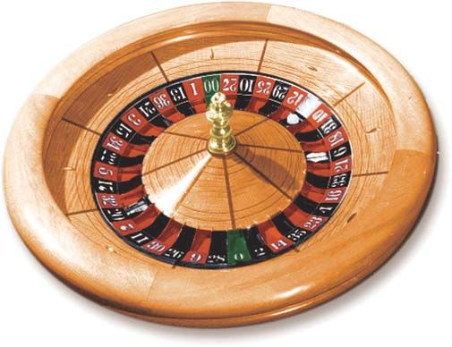
198                                                                  CROSON AND SUNDALI

different; individuals who believe in the hot hand believe not that a particular outcome is
hot (e.g. that the roulette wheel that has come up red in the past is likely to come up red
again), but that a particular person is hot. If an individual has won in the past (and is hot),
then whatever they choose to bet on is likely to win in the future.
   Gilovich, Vallone, and Tversky (1985) demonstrated both that individuals believe in
the hot hand in basketball shooting, and that basketball shooters’ probability of success is
indeed serially uncorrelated. Other evidence from the lab shows that subjects in a simulated
blackjack game bet more after a series of wins than they do after a series of losses, both
when betting on their own play and on the play of others (Chau and Phillips, 1995).
   The evidence for the hot hand from the field is weaker. Camerer (1989) compared odds in
the betting market for basketball teams with their actual performance and finds a small hot
hand bias. Bettors do appear to believe in the “hot team,” but the bias is small, not enough to
overcome the house edge in sports betting. Brown and Sauer (1993) use a different dataset
and analysis, but confirm the main findings of Camerer (1989).
   In more compelling evidence from the field, Clotfelter and Cook (1989) note the tendency
of gamblers to redeem winning lottery tickets for more tickets rather than for cash. This
behavior is also consistent with hot hand beliefs; since the individual has won previously
they are more likely to win again.
   The hot hand is thought to be caused by the illusion of control (Langer, 1975). Individuals
believe that they (or others) exert control over events that are in fact randomly determined.
We will test for hot hand beliefs in our data by looking at how betting behavior of individuals
change in response to wins and losses in roulette. In particular, hot hand beliefs predict that,
after a win, individuals will increase the number of bets they place and after a loss, decrease
them.3

2.     The data

In this study we use data from the field; individuals betting in a casino. In particular, we
will analyze bets placed at the game of roulette. Roulette is a useful game to use: it is
serially uncorrelated, unlike other casino games like blackjack or baccarat where previous
realizations influence future likelihoods. Also, roulette is an extremely popular game, thus
there is no shortage of data and the game is familiar to those playing it.

2.1.    Roulette

Roulette is played with a wheel and a betting layout. The wheel is divided into 38 even
sectors, numbered 1–36, plus 0 and 00 (in Europe, the wheel is divided into 37 sections,
1–36 plus 0). Each numbered space is colored red or black, with the exception of the 0 and
00, which are colored green. The wheel is arranged as shown in Figure 1, such that red and
black numbers alternate. The numbering on the wheel is not in numerical order but instead
the order as shown.
   Players arrive at the roulette table, and offer the dealer money (either cash or casino
chips). In exchange, they are given special roulette chips for betting at this wheel. These
chips are not valid anywhere else in the casino, and each player at the table has a unique
THE GAMBLER’S FALLACY AND THE HOT HAND                                                   199

Figure 1.   The wheel.

color of chips. Players bet by placing chips on a numbered layout, the wheel is spun and a
small white ball rolled around its edge. The ball lands on a particular number in the wheel,
which is the winning number for that round, and is announced publicly by the dealer. Next,
the dealer clears away all losing chips, players who had bet on the winning number (in some
configuration) are paid in their own-colored chips and a new round of betting begins.
   Figure 2 shows a typical layout. Unlike the wheel, the layout is arranged in numerical
order. Players can place their bets on varying places on the layout, covering a single number
or a combination of numbers located next to each other. All these bets pay the same, 36 for
one (35 to one) divided by the number of numbers covered by the bet. We count all these
betting combinations as “inside bets,” as they are bets placed inside the layout.
   In addition, bets like red/black, even/odd and low (1–18) and high (19–36) which pay
even money (2 for 1) and the thirds (1–12, 13–24 and 25–36) which pay 3 for 1 are outside
bets. If either 0 or 00 comes up, these outside bets lose.4
   Notice that all these bets have the same expected value, −5.26% on a double-zero wheel.5
If the wheel had no zeros, only 36 red or black numbers, the bets would be perfectly fair.

Figure 2.   The layout.
200                                                                CROSON AND SUNDALI

The zeros are thus sometimes referred to as the “house numbers,” even though players can
(and often do) bet on them.
   Since the house advantage on (almost) all bets at the wheel is the same, there is no
economic reason to bet one way or another (or for that matter, at all).6 In this sense our
data suffer from a similar limitation as Clotfelter and Cook’s (1991, 1993) who observed
lottery number choice in a fixed-payoff lottery. In this paper, we will compare the betting
behavior we observe against a benchmark of random betting and search for systematic and
significant deviations from that benchmark.

2.2.   Data and descriptive statistics

2.2.1. The data. The data was gathered from a large casino in Reno, Nevada.7 Casino
executives supplied the researchers with security videotapes for 18 hours of play of a single
roulette table. The videotapes consisted of three separate six-hour time blocks over a 3-day
period in July of 1998.8 The videotapes provided an overhead view of the roulette area.
The camera angle was focused on the roulette table, the roulette wheel, and the dealer. The
videotape was subtitled with a time counter. Note that while many casinos employ electronic
displays showing previous outcomes of the wheel, this casino had no such displays at the
time the data was collected. A research assistant was employed to view and record player
bet data from these videotapes.
   The videotape methodology made it possible to view all of bets made by each player
with a high degree of accuracy.9 However, while we could observe if a player bet on a
particular number, given the angle of the camera (from above), we could not observe how
many chips he or she bet on a particular number. Thus we simplified the data recording to
code a bet being placed, without mention of how much the bet was. In addition to coding
the bets placed on numbers, we separately coded for outside bets placed. After the assistant
recorded all of the bets from the 18 hours of videotape, one of the principal investigators
performed an audit check to insure accuracy.

2.2.2. Descriptive statistics: The wheel. Nine hundred and four spins of the roulette wheel
were captured in this data set (approximately 1 spin per minute). Table 1 shows the distri-
bution of outcomes (and bets) for numbers on the wheel.
   The expected frequency of a single number on a perfectly fair roulette wheel is 1/38 or
2.6%. In this sample the most frequent outcome was number 30 at 3.7%, the least frequent
outcome was number 26 at 1.7%. These data provide no evidence that the wheel is biased.10
Figure 3 shows the distribution of outcomes and bets for outside bets. Again, we cannot
conclude that the wheel is biased from this data.

2.2.3. Descriptive statistics: The bets. The data set included 139 players placing 24,131
bets. Table 2 presents some descriptive statistics of bets placed.
   Table 1 describes the bets placed by number. If players bet randomly, we would expect
them to bet on each number equally, thus 2.6% of the bets should fall on each number.
Figure 3 describes the frequency of observed outside bets.
THE GAMBLER’S FALLACY AND THE HOT HAND                                             201

Table 1.   Spin outcomes and player bets.

                Frequency                                % Outcome-   Frequency
Outcome          outcome        % Outcome   % Expected    expected       bet      % Bet

0/0                22              0.024      0.026        −0.002        354      0.016
 0                 25              0.028      0.026         0.001        442      0.020
 1                 23              0.025      0.026        −0.001        362      0.016
 2                 30              0.033      0.026         0.007        450      0.020
 3                 28              0.031      0.026         0.005        357      0.016
 4                 15              0.017      0.026        −0.010        375      0.017
 5                 28              0.031      0.026         0.005        636      0.028
 6                 20              0.022      0.026        −0.004        363      0.016
 7                 15              0.017      0.026        −0.010        682      0.030
 8                 26              0.029      0.026         0.002        633      0.028
 9                 23              0.025      0.026        −0.001        503      0.022
10                 24              0.027      0.026         0.000        484      0.021
11                 26              0.029      0.026         0.002        783      0.035
12                 21              0.023      0.026        −0.003        360      0.016
13                 21              0.023      0.026        −0.003        525      0.023
14                 27              0.030      0.026         0.004        649      0.029
15                 27              0.030      0.026         0.004        340      0.015
16                 25              0.028      0.026         0.001        643      0.029
17                 23              0.025      0.026        −0.001       1079      0.048
18                 23              0.025      0.026        −0.001        518      0.023
19                 30              0.033      0.026         0.007        595      0.026
20                 24              0.027      0.026         0.000        983      0.044
21                 26              0.029      0.026         0.002        447      0.020
22                 32              0.035      0.026         0.009        576      0.026
23                 24              0.027      0.026         0.000        746      0.033
24                 18              0.020      0.026        −0.006        461      0.020
25                 19              0.021      0.026        −0.005        521      0.023
26                 15              0.017      0.026        −0.010        703      0.031
27                 22              0.024      0.026        −0.002        490      0.022
28                 25              0.028      0.026         0.001        827      0.037
29                 23              0.025      0.026        −0.001        878      0.039
30                 33              0.037      0.026         0.010        695      0.031
31                 22              0.024      0.026        −0.002        664      0.029
32                 29              0.032      0.026         0.006        925      0.041
33                 17              0.019      0.026        −0.008        613      0.027
34                 29              0.032      0.026         0.006        597      0.027
35                 22              0.024      0.026        −0.002        627      0.028
36                 22              0.024      0.026        −0.002        641      0.028
202 CROSON AND SUNDALI
Table 2. Descriptive statistics of bets.
Mean Median High Low
Number of bets per player 174 114 1,412 1
Number of spins per player 18 11 132 1
Total number of bets 22,527 Inside
1,604 Outside
Figure 3. Outside outcomes and bets.
2.3. Gambler’s fallacy
We begin our analysis looking for the gambler’s fallacy, where observing a particular out-
come repeatedly in the past leads individuals to believe the opposite outcome is more likely
(is “due”). We focus on even-money outside bets, Red/Black, Odd/Even, and Low/High.
We classify a bet as consistent with the gambler’s fallacy if it was placed on an outcome
that is against a streak of length n. A streak of length n is simply the number of times a
particular outcome has appeared consecutively in the past.
For example, if a red number has won the last four trials, this is counted as a streak of
length four. At this point, a bet on black would be counted as a gambler’s fallacy bet. A
similar logic would categorize a bet on an even number after four odd numbers had appeared.
Figure 4 describes the frequency of gambler’s fallacy bets after streaks of varying length.
As shown in Figure 4, there were 531 bets placed on one of the even-money outside bets
after having observed at least one spin. Of these 531 bets, 255 (48%) were gambler’s fallacyTHE GAMBLER’S FALLACY AND THE HOT HAND 203 Figure 4. Proportion of gambler’s fallacy outside bets after a streak of at least length N . bets (against the previously-observed outcome) and 276 (52%) were with the previously- observed outcome. The next set of columns considers streaks of length two. Of those 258 bets that were placed on outside bets after streaks of length two, 51% were gambler’s fallacy bets. A binomial test at each level of streak compares the actual bets observed with the baseline hypothesis of 50%. There are no significant differences after streaks of length one, two, three or four. However, for streaks of length 5 ( p < .05) and for streaks of length 6 and above ( p < .01), there is evidence consistent with gambler’s fallacy play. Thus we find statistical evidence that individuals bet consistently with gambler’s fallacy beliefs. After streaks of 5 (or more) outcomes of a particular type, gamblers are significantly more likely to bet against the streak than to bet with it. This result is consistent with the models of Rabin (2002) and Mullainathan (2002). As can be seen in Figure 4, as the length of the streak increases the proportion of gambler’s fallacy bets increases as well. After streaks of 6 or more, 85% of bets are consistent with the gambler’s fallacy. 2.4. Hot hand Our second set of analyses investigates whether individual’s behavior is consistent with hot hand beliefs. To do this, we analyze whether gamblers bet on more or fewer numbers in response to previous wins and losses. The most extreme reduction of bets possible is to stop betting altogether (to leave the table). Of our 139 subjects, 80% (111) quit playing after losing on a spin while only 20% (28) quit after winning. This behavior is consistent with the hot hand; after a win players are likely to keep playing (because they’re hot). On the other hand, quitting is a very discrete measure of beliefs about hotness. A more continuous measure might involve the number of bets placed on a given spin as a function
204                                                                            CROSON AND SUNDALI

                     Table 3.     Number of outside bets placed.

                                                   Average          St. dev.    N

                     First spin                      0.48            0.71       139
                     Won prior spin outside          1.53            0.63      454
                     Lost prior spin outside         1.38            0.57       608

of the outcome of the previous spin. Table 3 presents the average number of outside bets
placed by gamblers on the initial trial and after a win or loss on an outside bet on the
previous spin.11 We count the number of times these outside bets were placed, averaged
over individuals and types of spins (first, previously winning or previously losing). We
exclude observations when individuals remained at the table but had not previously placed
an outside bet. Only individuals who placed bets are included in this analysis; individuals
who left the table are not counted as having placed zero bets but instead excluded.
   After an outside bet win (which occurred 454 times in our data set), individuals place
on average 1.53 outside bets. After an outside bet loss (which occurred 608 times in our
data set), individuals placed on average 1.38 outside bets. A regression run on the number
of bets placed as a function of winning or losing shows a significant, though small, impact
( p < .05). Thus the data provide evidence of a hot hand in betting behavior. Individuals place
more outside bets when they have previously won than when they have previously lost.12
   Table 4 presents the average number of bets placed on numbers by gamblers after an inside
win or loss on the previous spin. As before, we exclude observations when individuals were
at the table but had not previously placed an inside bet and only individuals who placed
bets are included in this analysis; individuals who left the table are not counted as having
placed zero bets but instead excluded.
   There were 570 instances where an individual had won an inside bet on the previous spin.
In this case, players bet on an average 13.62 numbers. There were 1487 instances where
an individual had lost on the previous spin. In this case, players bet on an average of 9.21
numbers. A regression run on the number of bets placed as a function of winning or losing
shows a significant impact ( p < .05).13 Thus the data on inside bets also provides evidence
for the hot hand.14
   We have enough observations of inside bets for a more complex regression. The dependent
variable is the number of inside bets placed by person i on spin t, n it . The independent
variables are an indicator variable equal to 1 if the person had won on the previous spin and

                     Table 4.     Number of inside bets placed.

                                                  Average          St. dev.     N

                     First spin                      7.63           6.12        139
                     Won prior spin inside          13.62           6.60        570
                     Lost prior spin inside          9.21           5.35       1487
THE GAMBLER’S FALLACY AND THE HOT HAND 205
Table 5. Hot hand regression.
Intercept 1.63∗∗ −1.83
Win previous trial 1.09∗∗ 0.99∗∗
# bets placed last spin 0.58∗∗ 0.27∗∗
# bets placed first trial 0.23∗∗ 2.07∗∗
Individual dummies No Yes
R2 (adjusted) .64 .64
∗∗ p < 0.01; ∗p < 0.05; ∧p < 0.10.
0 otherwise (wonit−1 ), the number of bets the individual had placed on the previous spin
(numberit−1 ) and the number of bets the individual had placed on their first trial as a control
for individual differences (firsti ). As before, individuals who have left the table before spin
t (who bet zero on spin t) are excluded. The regression equation is thus
n it = α0 + α1 wonit−1 + α2 numberit−1 + α3 firsti + ε
Results from this regression are shown in Table 5. The second column adds individual
dummy variables for each person in our dataset.
As Table 5 indicates, winning a bet in trial t − 1 significantly increases the number of
bets placed in trial t, consistent with the hot hand bias and the results of Camerer (1989)
and Brown and Sauer (1993).15
3. Conclusion and discussion
This paper uses observational data to investigate the existence and impact of two statistical
illusions; the gambler’s fallacy and the hot hand. These biases and their resulting behaviors
have been observed in the lab; we find evidence for these illusions in the field using data
from casino gambling. Our paper makes two important contributions to the behavioral
economics literature. First, we provide field data to examine the existence of biases in the
perception of sequences of gambles. Second, unlike previous research with field data, we
have observations of individual’s behavior, enabling us to test behavior directly rather than
looking more indirectly at market outcomes, as in Camerer (1989) and Brown and Sauer
(1993). A related paper (Sundali and Croson, 2002) provides an even more disaggregated
analysis of this data and identifies heterogeneity in the existence and strength of these biases
in different individuals.
Our data demonstrate that gamblers bet in accordance with the gambler’s fallacy. After
observing a streak of 5 or more occurrences of a particular outcome, they place significantly
more bets against the streak than with the streak. This result is consistent with the models
of Mullainathan (2002) and Rabin (2002). Our data also demonstrate that gamblers act in
a way consistent with the hot hand; they bet on more numbers after winning than after
losing.206 CROSON AND SUNDALI These results are consistent with those previously observed in the lab. That these obser- vations are robust when generalized from lab to field is reassuring. However, the limitations inherent in field data admit of alternative interpretations of some of our results. For example, the hot hand result may be explained by an income or house money effect; individuals bet on more numbers after they have won not because they believe that they (personally) are more likely to win again but because they’re richer, or playing with the house’s money. A similar explanation, suggested by a helpful referee, involves individuals betting some fixed fraction of the chips gamblers have in front of them. While we cannot rule out these explanations using field data, previous lab studies have controlled for them (e.g. Chau and Phillips, 1995). Future lab studies could be designed to do so as well; by manipulating the win/loss history while keeping the current income constant we could test the effect of history on behavior without the confounding factor of income. Similarly, eliciting probability judgments after each trial would provide direct evidence of biased beliefs in a way that is not possible in the field. A second important limitation of this (and related) research has to do with the cost of exhibiting these biases. In roulette, as in most casino games, the odds of winning or losing are relatively constant independent of how you bet. For example, in craps the house edge from betting the “pass” line is 1.41% and the “don’t pass” line is 1.40%. In blackjack the house advantage does not change as the size of the bet changes. Thus the decision of whether to bet pass or don’t pass, or of how much to bet at blackjack, is not a costly one in terms of expected value. Thus these settings are ones where biased beliefs are most likely to develop and persist. These limitations suggest the need for further research combining empirical and lab data in a way that we were prevented from accomplishing here. After observing individual decisions in the field, follow-up lab studies or surveys can help to tease apart these alternative explanations of behavior. Empirical data from financial decision-making could be combined with survey data in a similar way. Other future projects might involve data from other iid casino games (e.g. craps, slot machines) both to replicate our current findings and to identify differences between the games. Almost every decision we make involves uncertainty in some way. It has been amply demonstrated by lab experiments (and some previous empirical papers) that we suffer from biases in uncertain decision situations. This paper uses data from individuals gambling in a casino to test for the presence of these biases in a naturally-occurring environment. The gambling biases we observe are consistent with previously-observed departures from rationality in the lab and in the field. Acknowledgments The authors thank Eric Gold for substantial contributions in earlier stages of this project. Thanks also to Jeremy Bagai, Dr. Klaus von Colorist, Bradley Ruffle, Paul Slovic, Willem Wagenaar, participants of the J/DM and ESA conferences, at the Conference on Gambling and Risk Taking and at seminars at Wharton, Caltech and INSEAD for their comments on this paper. Special thanks to the Institute for the Study of Gambling and Commercial Gaming for industry contacts which resulted in the acquisition of the observational data reported
THE GAMBLER’S FALLACY AND THE HOT HAND                                                                           207

here. Financial support from NSF SES 98-76079-001 is also gratefully acknowledged. All
remaining errors are ours.

Notes

 1. While biased roulette wheels, loaded dice and stacked decks of cards do indeed exist, major casinos in the
    US are heavily regulated, subject to periodic auditing and severe penalties (loss of gaming license, fines and
    jail time) for offering rigged games. Furthermore, gambling devices which are nonrandom (or predictable)
    represent financial liabilities to the casino, as informed patrons can take advantage of the better-than-expected
    odds.
 2. Although, as one reader points out, the production of a random sequence is a different task than predicting or
    perceiving a random sequence.
 3. There are alternative explanations for these behaviors. For example, wealth effects or house money effects
    might cause an increase in betting after a win. In our empirical data we will not be able to distinguish between
    these alternative explanations although previous lab experiments have done so.
 4. This rule, that outside bets lose when 0 or 00 comes up, varies somewhat between casinos and, in particular,
    between the US and Europe. Sometimes only half of the outside bet is lost, with the remainder being paid
    directly to the player. In other casinos, the outside bet is held “in prison.” The bet must remain unchanged until
    the next spin, where it then either wins or loses depending on the outcome of the wheel. These rule variations
    impact the house advantage in the game. In our data, outside bets are lost when 0 or 00 appears.
 5. This statement is not strictly true. There is, in fact, one bet has a house advantage of 7.89%. The bet involves
    placing a chip on the outside corner of the layout between 0 and 1. The bet wins if 0, 00, 1, 2 or 3 appears, but
    pays only 6 for 1 (as though the bet were covering 6 numbers instead of 5). We observed only 75 instances of
    this bet being placed (out of 24,131 bets). Only 11 different individuals placed this bet (out of 139 identifiable
    individuals in our data), and of them, only 6 placed this bet more than twice.
 6. Because of this the incentive to learn how to play roulette may be dampened. On the other hand, there remains
    an incentive to learn how to place the bets (the etiquette of the game) and how much each bet pays (to make
    sure the dealer is paying you correctly).
 7. A casino in Washoe County, Nevada is classified as “large” by the Nevada Gaming Control Board if total
    (yearly) gaming revenues for the property exceeds $36 million.
 8. The three time blocks were from 4:00 p.m. to 10:00 p.m., 8:00 p.m. to 2:00 a.m., and 10:00 p.m. to 4:00 a.m.
    These time blocks were appropriate since the majority of gaming business is done in the evening hours.
 9. Players were identified based upon the color of the chips being used to bet, the player’s location at the table,
    and any distinct characteristics of the player’s hand or arm such as appearance, jewelry, clothing, tattoos, etc.
    Players who ran out of chips and immediately bought more (of the same color) were coded as the same player.
    Players who ran out of chips and did not immediately buy more were coded as having left the table. When
    money was again exchanged for chips of that particular color, we assumed a new player had joined the table.
10. Ethier (1982) calculates the number of observations necessary to detect a bias in the wheel.
11. We follow Wagenaar (1988) in defining hot hand as having won the previous spin and being otherwise
    independent of longer, lagged history. One might imagine extending this notion of hot hand to include (more
    restrictively) having won the previous N spins or (less restrictively) having won on one of the previous N
    spins.
12. A similar pattern can be found looking at the impact of all previous bets on current outside bets. After winning
    either an inside or an outside bet, individuals placed an average of 0.85 outside bets. After losing, they placed
    an average of 0.50 outside bets. These differences are also significant at p < .05.
13. A similar pattern can be found looking at the impact of all previous bets on current inside bets. After winning
    either an inside or an outside bet, individuals placed an average of 10.30 inside bets. After losing, they placed
    an average of 8.21 inside bets. These differences are also significant at p < .05
14. As noted elsewhere in the paper, there are competing explanations of behavior which would be consistent
    with this data. One such explanation, suggested by a helpful referee, is that gamblers bet a fixed percentage
    of the chips they have remaining in front of them. If this is the case, they would also bet more after a win
208 CROSON AND SUNDALI
and less after a loss. A more thorough discussion of alternative explanations for our data can be found in the
discussion section.
15. A similar regression of the change in the number of bets placed (n it − n it−1 ) on whether the individual won
last spin and the number of bets they placed on the first spin also yields a positive and significant coefficient
on past wins.
References
Brown, William and Raymond Sauer. (1993). “Does the Basketball Market Believe in the Hot Hand? Comment,”
American Economic Review 83, 1377–1386.
Cahart, Mark. (1997). “On Persistence in Mutual Fund Performance,” Journal of Finance 52, 57–82.
Camerer, Colin. (1989). “Does the Basketball Market Believe in the ‘Hot Hand’?” American Economic Review
79, 1257–1261.
Camerer, Colin. (1998). “Can Asset Markets be Manipulated? A Field Experiment with Racetrack Betting,”
Journal of Political Economy 106, 457–482.
Chau, Albert and James Phillips. (1995). “Effects of Perceived Control Upon Wagering and Attributions in
Computer Blackjack,” The Journal of General Psychology 122, 253–269.
Clotfelter, Charles and Phil Cook. (1989). Selling Hope: State Lotteries in America. Cambridge: Harvard University
Press.
Clotfelter, Charles and Phil Cook. (1991). “Lotteries in the Real World,” Journal of Risk and Uncertainty 4,
227–232.
Clotfelter, Charles and Phil Cook. (1993). “The ‘Gambler’s Fallacy’ in Lottery Play,” Management Science 39,
1521–1525.
Estes, William. (1964). “Probability Learning.” In A.W. Melton (ed.), Categories of Human Learning. New York:
Academic Press.
Ethier, Stuart. (1982). “Testing for Favorable Numbers on a Roulette Wheel,” Journal of the American Statistical
Association 77, 660–665.
Gilovich, Thomas, Robert Vallone and Amos Tversky. (1985). “The Hot Hand in Basketball: On the Misperception
of Random Sequences,” Cognitive Psychology 17, 295–314.
Golec, Joseph and Murray Tamarkin. (1998). “Bettors Love Skewness, Not Risk, at the Horse Track.” Journal of
Political Economy 106, 205–225.
Langer, Ellen. (1975). “The Illusion of Control,” Journal of Personality and Social Psychology 32, 311–328.
Laplace, Pierre. (1820: 1951) Philosophical Essays on Probabilities, translated by F. W. Truscott and F. L. Emory.
New York: Dover.
Metzger, Mary. (1984). “Biases in Betting: An Application of Laboratory Findings,” Psychological Reports 56,
883–888.
Mullainathan, Sendhil. (2002). “Thinking Through Categories,” Working Paper, Department of Economics,
Massachusetts Institute of Technology.
Odean, Terrence. (1998). “Are Investors Reluctant to Realize their Losses?” Journal of Finance 53, 1775–1789.
Quandt, Richard. (1986). “Betting and Equilibrium,” Quarterly Journal of Economics 101, 201–207.
Rabin, Matthew. (2002). “Inference by Believers in the Law of Small Numbers,” Quarterly Journal of Economics
157, 775–816.
Ritov, Ilana and Jonathan Baron. (1992). “Status Quo and Omission Bias,” Journal of Risk and Uncertainty 5,
49–61.
Samuelson, William and Richard Zeckhauser. (1988). “Status Quo Bias in Decision Making,” Journal of Risk and
Uncertainty 1, 7–59.
Shefrin, Hersh and Meir Statman. (1985). “The Disposition to Sell Winners Too Early and Ride Losers Too Long:
Theory and Evidence,” Journal of Finance 40, 777–790.
Sirri, Erik and Peter Tufano. (1998). “Costly Search and Mutual Fund Flows,” Journal of Finance 53, 1589–
1622.
Sundali, James and Rachel Croson. (2004). “Biases in Casino Betting: The Hot Hand and the Gambler’s Fallacy,”
Working Paper, The Wharton School, University of Pennsylvania.THE GAMBLER’S FALLACY AND THE HOT HAND 209 Terrell, Dek. (1994). “A Test of the Gambler’s Fallacy: Evidence from Pari-Mutuel Games,” Journal of Risk and Uncertainty 8, 309–317. Terrell, Dek. (1998). “Biases in Assessments of Probabilities: New Evidence from Greyhound Races,” Journal of Risk and Uncertainty 17, 151–166. Terrell, Dek and Amy Farmer. (1996). “Optimal Betting and Efficiency in Parimutuel Betting Markets with Information Costs,” The Economic Journal 106, 846–868. Tversky, Amos and Daniel Kahneman. (1971). “Belief in the Law of Small Numbers,” Psychological Bulletin 76, 105–110. Wagenaar, Wilhelm. (1988). Paradoxes of Gambling Behavior. London: Lawrence Erlbaum. Walker, Mark and John Wooders. (2001). “Minimax Play at Wimbledon,” American Economic Review 91, 1521– 1538.
You can also read