THE HIGH LATITUDE MARINE HEAT WAVE OF 2016 AND ITS IMPACTS ON ALASKA
←
→
Page content transcription
If your browser does not render page correctly, please read the page content below
8. THE HIGH LATITUDE MARINE HEAT WAVE OF 2016 AND
                      ITS IMPACTS ON ALASKA

         John E. Walsh, Richard L. Thoman, Uma S. Bhatt, Peter A. Bieniek, Brian Brettschneider,
       Michael Brubaker, Seth Danielson, Rick L ader, Florence Fetterer, Kris Holderied, K atrin Iken,
                           Andy Mahoney, Molly McCammon, and James Partain

                 The 2016 Alaska marine heat wave was unprecedented in terms of sea surface temperatures
                 and ocean heat content, and CMIP5 data suggest human-induced climate change has greatly
                                            increased the risk of such anomalies.

     Earth System Observations. The Gulf of Alaska (GOA)               The consensus of previous studies is that atmo-
     and Bering Sea have been anomalously warm for                 spheric circulation anomalies played a key role in
     several years with the warmth peaking in 2016.                initiating and maintaining the North Pacific “blob”
     As a consequence of the high marine heat content              of warm water (Bond et al. 2015). Unusually high pres-
     (HC) and SSTs, coastal areas of Alaska had their              sure south of the Gulf of Alaska reduced heat loss to
     warmest winter–spring of record in 2016 (Walsh et             the atmosphere and also reduced cold advection over
     al. 2017) and earliest river ice breakup for multiple         the region. Forcing of the atmospheric anomalies has
     Alaska rivers (www.weather.gov/aprfc/breakupDB).              been linked to SST anomalies in the western tropical
     Observed marine warmth, impacts on the marine                 Pacific Ocean (Seager et al. 2015) and to decadal-scale
     ecosystem, and an attribution analysis using CMIP5            modes of North Pacific Ocean variability (Di Lorenzo
     models are presented here.                                    and Mantua 2016). Lee et al. (2015) have argued that
         The marine heat wave was first noted over deep            sea ice anomalies also contributed to the atmospheric
     waters of the northeastern Pacific Ocean in January           circulation anomalies in 2013/14. By contrast, the
     2014 (Freeland 2014; Bond et al. 2015); anomalous             winter of 2015/16 was characterized by negative sea
     temperatures at coastal GOA stations arrived vari-            level pressure anomalies of more than 12 hPa centered
     ously between January and June. Warm temperature              in the eastern Bering Sea (Fig. ES8.1d). The associated
     anomalies were confined to the top 100 meters until           northward airflow evident throughout the depth of
     late 2014, after which they penetrated to depths of 300       the atmosphere (Fig. ES8.1b) likely drove lingering
     meters and reached strengths greater than 2 standard          heat from the blob into the GOA and Bering Sea
     deviations (Roemmich and Gilson 2009).                        regions. An unusually deep Aleutian low is a typical
                                                                   feature of the El Niño conditions that characterized
AFFILIATIONS: Walsh and B rettschneider—Alaska Center
for Climate Assessment and Policy, University of Alaska,
                                                                   early 2016 (Walsh et al. 2017).
Fairbanks, Alaska; Thoman —NOAA/National Weather Service               The positive HC anomalies (Fig. 8.1a) reached an
Alaska, Fairbanks, Alaska; B hatt—Geophysical Institute, and       extreme in 2016 for the GOA and Bering Sea (Figs.
Department of Atmospheric Sciences, University of Alaska,          8.1d,e), with most of the region ranking in the top five
Fairbanks, Alaska; Mahoney—Geophysical Institute, University of
Alaska, Fairbanks, Alaska; L ader—International Arctic Research
                                                                   warmest HCs of record (Fig. ES8.2a). Oceanic tem-
Center, University of Alaska, Fairbanks, Alaska; B ieniek—Alaska   peratures are from GODAS (Saha et al. 2006), NCEP’s
Climate Science Center, University of Alaska, Fairbanks, Alaska;   high-resolution ocean analysis. HC was calculated by
B rubaker—Alaska Native Tribal Health Consortium, Anchorage,       integrating ocean temperature (°C) from the surface
Alaska; Danielson and Iken —College of Fisheries and Ocean
Sciences, University of Alaska, Fairbanks, Alaska; Fetterer—
                                                                   to 300 meters or the bottom of each model water
NSIDC and NOAA/NESDIS National Centers for Environmental           column. This value was then divided by the depth of
Information, Boulder, Colorado; Holderied —NOAA/National           its respective water column, the 1981–2010 mean was
Ocean Service, National Centers for Coastal Ocean Science,         removed, and the quantity was normalized to allow
Seldovia, Alaska; McCammon —Alaska Ocean Observing System,
Anchorage, Alaska; Partain —NOAA/NESDIS National Centers
                                                                   comparison between the Bering Sea (51°–64.5°N,
for Environmental Information, Anchorage, Alaska                   180°–160°W) and GOA (50°–60°N, 150°–130°W)
DOI:10.1175/BAMS-D-17-0105.1                                       regions (Figs. 8.1d,e).
A supplement to this article is available online (10.1175
/BAMS-D-17-0105.2)

     AMERICAN METEOROLOGICAL SOCIETY                                                                 JANUARY 2018         | S39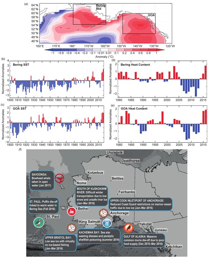
Fig. 8.1. (a) Jan–Dec 2016 ocean heat content anomaly (°C) from the surface to 300 m or bottom of ocean
column. Boxes outline GOA and Bering Sea regions. Normalized area-weighted SST anomalies for (b) Bering
Sea and (c) GOA. Normalized area-weighted heat content anomalies for (d) Bering Sea and (e) GOA. (f) Select
impacts of 2016 marine heat in Alaska waters.

      Normalized SST anomalies from 1900 provide          warmest in the GOA (Figs. 8.1b,c) where 2015 was
    context for the anomalies. The 2016 SSTs were the     warmest. SSTs were anomalously warm starting in
    warmest on record for the Bering Sea and the second   2012 (Weller et al. 2015), and most of the GOA and

S40 |      JANAURY 2018
Bering Sea ranked in the top five SSTs of record (Fig. observers noted changes in seasonality, weather,
ES8.2b). SST data are from NOAA’s Extended Recon- ocean conditions, plants, and wildlife, which chal-
structed Sea Surface Temperature dataset, version 4 lenge people engaged in subsistence and commercial
(Huang et al. 2014), and anomalies use the 1981–2010 activities with increased variability and uncertainty.
mean. Negative anomalies greater than 2 sigma are The lack of winter sea ice in western Alaska delayed
evident in both regions from 2006–13. or prevented ice-based harvesting of fish, crab, seal,
The warming was primarily confined to the inner and whale. For shellfish harvests, the warm waters
GOA shelf in September 2014, suggesting that heat translated into persistent high levels of harmful algae
was advected along-shore within the Alaska Coastal across the GOA and North Pacific as far west as the
Current. By spring 2015 the shelf was uniformly warm Aleutian Islands, with concerns about food safety
and water remained 1°–2°C warmer than normal extending to the Bering Strait.
through September 2016. This heat was accompanied
by surface mixed layer shoaling and a strengthening Attribution. The role of anthropogenic climate change
of the near-surface stratification, impacting nutrient in the marine heat wave of 2016 was assessed through
availability and the ecosystem. an evaluation of CMIP5 model output. Attribution
was estimated by comparing SSTs and HC in 60-
Impacts. Ecological and societal impacts of the 2016 year segments (to resolve relevant decadal variability
marine heat wave are complex but unequivocal. such as the Pacific decadal oscillation; PDO) from
Some marine ecological impacts resulted from the present and preindustrial climate simulations. Five
multiyear nature of the marine heat wave, so cannot CMIP5 models were selected (see online supplement
be attributed solely to the 2016 event. material; Walsh et al. 2017b, manuscript submitted
The consequences of this persistent warming to Environ. Modell. Software): CCSM4, GFDL-CM3,
were felt through the entire marine food web. The GISS-E2-R, IPSL-CM5A-LR, and MRI-CGCM3. The
warm conditions favored some phytoplankton spe- models’ trends of SST over the 1900–2005 historical
cies, and one of the largest harmful algal blooms on simulations ranged from 0.27° to 0.52°C century−1
record reached the Alaska coast in 2015 (Peterson et (mean = 0.41°C) for the Bering Sea and 0.22° to
al. 2016a). Kachemak Bay had uncommon paralytic 0.90°C century−1 (mean = 0.46°C) for the GOA. The
shellfish poisoning events and oyster farm closures corresponding observational values from Figs. 8.1b,c
in 2015 and 2016. Copepods, the crustaceans that are 0.70° and 0.84°C century−1 for the Bering Sea and
form the cornerstone of the open ocean food web, GOA. If the models’ century-scale trends represent
had a higher abundance of smaller species, which the anthropogenic forcing signal, then one may ar-
provide less nutritious food source to higher trophic gue that the larger values of the observed trends are
levels, including forage fish. The occurrence of more partially attributable to internal variability.
southern copepod species in the GOA likely resulted For the attribution analysis, the present climate pe-
from the anomalous warmth (Kintisch 2015; Peterson riod is centered on 2016 and incorporates the histori-
et al. 2016b). cal simulation (1987–2005) and RCP8.5 (2006–46),
The dramatic mortality events in seabird species which is the current trajectory of climate forcing,
such as common murres (Uria aalge) in 2015/16 (tens while the preindustrial climate incorporates a random
of thousands of dead birds counted) were attributed 60-year period from each model. Monthly HC was
to starvation and presumed to be a result of warming- calculated using ocean potential temperatures with a
induced effects on food supply (H. Renner 2017, U.S. procedure similar to that used for GODAS. The SSTs
Fish and Wildlife Service, personal communication). and HCs were then interpolated to the GODAS grid,
Increased occurrences of diseases were also observed, annual averages were computed, and area-weighted
including sea star wasting disease, first recognized averages were extracted over the Bering Sea and GOA.
in Kachemak Bay in 2015. (K. Iken 2017, personal This yielded 60-year time series for each region,
observations; Fig. 8.1f). model, and variable (present and preindustrial).
Over 100 observations of impacts on communities Annual values of SST and HC are warmer in GOA
across Alaska were posted to the Local Environmen- than the Bering Sea. Normalized anomalies using a
tal Observer (LEO) network (http://leonetwork.org) 1987–2016 base period were used to account for differ-
between October 2013 and December 2016. These ences in means. For SST and HC the present climate
impacts relate to changes in the acquisition, pres- has increasing trends while the preindustrial does not
ervation, quality, and quantity of wild foods. Local (Figs. 8.2a,b). In all cases the preindustrial climate is
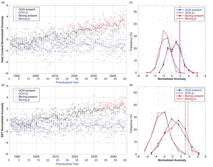
AMERICAN METEOROLOGICAL SOCIETY JANUARY 2018 | S41Fig. 8.2. Normalized anomalies of (a) heat content and (b) SSTs for the present (black) and preindustrial (blue)
climate of the GOA (circle and plus) and Bering Sea (triangle and x) regions from the five model ensembles.
Anomalies exceeding 2016 value are in red (shapes as indicated), and the ensemble/region means are shown by
the solid lines. Mean probability distributions (%) of (c) heat content and (d) SSTs from the model ensembles;
solid (open) circles indicate present (preindustrial) climate for the GOA (blue) and Bering Sea (red). Spread
of individual models is shown by the smaller, corresponding open/closed circles. Dashed vertical lines show the
2016 anomalies: GOA (blue), Bering Sea (red).
generally cooler with no extreme positive anomalies preindustrial climate never reached the 2016 observed
comparable to the present climate (Figs. 8.2c,d). magnitude.
Each model/variable/region was compared with In this analysis the fraction of attributable risk
its corresponding 2016 observed normalized anomaly (FAR; Stott et al. 2004; NASEM 2016) was computed
value (see red coloring in Figs. 8.2a,b and vertical as FAR = 1 − Probpreindustrial/Probpresent with the prob-
dashed lines in Figs. 8.2c,d). The preindustrial period ability being the exceedance of the observed 2016
had few cases meeting or exceeding the 2016 anomaly normalized anomaly. Bering Sea SSTs had FAR = 1
for any region or variable, while the present climate for all cases, while the GOA’s FARs were 0.88–1 for
had many more, especially later in the period. For SST and 0.82–1 for HC (but most models had FAR = 1,
HC the number of years each model exceeded the i.e., no instances of 2016-like anomalies in the prein-
2016 anomaly ranged from 11 to 20 (0–2) cases in the dustrial climate).
present (preindustrial) climate for GOA and 16–24
(0) for Bering Sea. Fewer cases reached 2016 values Conclusion. The warmth of the Bering Sea in 2016
in SSTs, with 5–18 (0–1) for GOA and 4–11 (0) for was unprecedented in the historical record, and
Bering Sea. For both variables the Bering Sea region’s the warmth of the GOA nearly so. The FAR values
S42 | JANAURY 2018based on an ensemble of five global climate models Huang, B., and Coauthors, 2014: Extended reconstruct-
indicate that the 2016 warm ocean anomalies cannot ed sea surface temperature version 4 (ERSST.v4): Part
be explained without anthropogenic climate warm- I. Upgrades and intercomparisons. J. Climate, 28,
ing, although the region’s large internal variability 911–930, doi:10.1175/JCLI-D-14-00006.1
was also a contributing factor (Fig. 8.1 and online Lee, M.-Y., C.-C. Hong and H.-H. Hsu, 2015: Compound-
supplement material). A strong El Niño with a posi- ing effects of warm sea surface temperature and re-
tive PDO (warm) phase, together with precondition- duced sea ice extent on the extreme circulation over
ing of the waters during 2014/15 and the anomalous the extratropical North Pacific and North America
atmospheric circulation of early 2016, made for a during the 2013-2014 boreal winter. Geophys. Res.
“perfect storm” of marine heating around Alaska. Lett., 42, 1612–1618, doi:10.1002/2014GL062956.
Both anthropogenic forcing and internal variability Kintisch, E., 2015: ‘The Blob’ invades Pacific, flummox-
were necessary for the extreme warmth of the sub- ing climate experts. Science, 348, 17–18.
arctic seas. Our conclusions are consistent with and NASEM, 2016: Attribution of extreme weather events in
extend previous findings concerning the 2014 warm the context of climate change. National Academies
SST anomalies in the northeast Pacific (Weller et al. Press, 186 pp., doi:10.17226/21852.
2015). Additionally, the trajectory of the present cli- Peterson, W., N. Bond, and M. Robert, 2016a: The
mate with RCP8.5 indicates that SST and HC extreme blob (part three): Going, going, gone? PICES Press,
anomalies like 2016 will become common in the 24 (1), 46–48. [Available online at https://pices.int
coming decades. Given the many impacts of the 2016 /publications/pices_press/volume24/PPJan2016.pdf.]
anomaly, the future climate projected here will result —, —, and —, 2016b: The blob is gone but has
in a profound shift for people, systems, and species morphed into a strongly positive PDO/SST pattern.
when such warm ocean temperatures become com- PICES Press, 24 (2), 46–47, 50. [Available online at
mon and not extreme in the GOA and Bering regions. http://meetings.pices.int/publications/pices-press
/volume24/issue2/PPJuly2016.pdf.]
ACKNOWLEDGMENTS. This work was sup- Roemmich, D., and J. Gilson, 2009: The 2004–2008
ported by the Alaska Climate Science Center through mean and annual cycle of temperature, salinity,
Cooperative Agreement G10AC00588 from the USGS and steric height in the global ocean from the Argo
and by the NOAA Climate Program Office through Program. Progr. Oceanogr., 82, 81–100, doi:10.1016
Grant NA16OAR4310162 to the Alaska Center for /j.pocean.2009.03.004.
Climate Assessment and Policy. The papers contents Saha, S., and Coauthors, 2006: The NCEP climate fore-
are solely the responsibility of the authors and do not cast system. J. Climate, 19, 3483–3517, doi:10.1175
necessarily represent the official views of the USGS. /JCLI3812.1.
Seager, R., M. Hoerling, S. Schubert, H. Wang, B. Lyon,
A. Kumar, J. Nakamura, and N. Henderson, 2015:
Causes of the 2011–14 California drought. J. Climate,
28, 6997–7024, doi:10.1175/JCLI-D-14-00860.1.
Stott, P., D. Stone, and M. Allen, 2004: Human contribu-
tion to the European heatwave of 2003. Nature, 432,
REFERENCES 610–614, doi:10.1038/nature03089.
Walsh, J. E., P. A. Bieniek, B. Brettschneider, E. S. Eu-
Bond, N. A., M. F. Cronin, H. Freeland, and N. Mantua skirchen, R. Lader, and R. L. Thoman, 2017: The
2015: Causes and impacts of the 2014 warm anomaly exceptionally warm winter of 2015-16 in Alaska: At-
in the NE Pacific. Geophys. Res. Lett., 42, 3414–3420, tribution and anticipation. J. Climate, 30, 2069–2088,
doi:10.1002/2015GL063306. doi:10.1175/JCLI-D-16-0473.1.
Di Lorenzo, E., and N. Mantua, 2016: Multi-year persis- Weller, E., S.-K. Min, D. Lee, W. Cai, S.-W. Yeh, and J.-S.
tence of the 2014/15 North Pacific marine heatwave. Kug, 2015: Human contribution to the 2014 record
Nat. Climate Change, 6, 1042–1047, doi:10.1038 high sea surface temperatures over the western
/nclimate3082. tropical and northeast Pacific Ocean [in “Explaining
Freeland, H., 2014: Something odd in the Gulf of Alaska, Extreme Events of 2014 from a Climate Perspec-
February 2014. CMOS Bulletin SCMO, 42, 57–59. tive”]. Bull. Amer. Meteor. Soc., 96 (12), S100–S104,
[Available online at http://cmos.ca/uploaded/web doi:10.1175/BAMS-D-15-00055.1.
/members/Bulletin/Vol_42/b4202.pdf.]
AMERICAN METEOROLOGICAL SOCIETY JANUARY 2018 | S43You can also read