The Impact of Interest Rate, Exchange Rate and European Business Climate on Economic Growth in Romania: An ARDL Approach with Structural Breaks
←
→
Page content transcription
If your browser does not render page correctly, please read the page content below
sustainability

Article
The Impact of Interest Rate, Exchange Rate and
European Business Climate on Economic Growth in
Romania: An ARDL Approach with Structural Breaks
Mariana Hatmanu 1, *, Cristina Cautisanu 2              and Mihaela Ifrim 1
 1    Faculty of Economics and Business Administration, Alexandru Ioan Cuza University of Iasi,
      700505 Iasi, Romania; mihaela.ifrim@uaic.ro
 2    CERNESIM Environmental Research Center, Alexandru Ioan Cuza University of Iasi, 700505 Iasi, Romania;
      cristina.cautisanu@uaic.ro
 *    Correspondence: mariana.hatmanu@uaic.ro

 Received: 5 February 2020; Accepted: 28 March 2020; Published: 1 April 2020

 Abstract: The role of the interest and exchange rates in sustaining economic growth has been a highly
 researched subject. Therefore, this study examines the influence of the monetary policy interest rate,
 the real exchange rate and the business climate in the Euro area on the economic growth in Romania.
 For this purpose, we have applied a pre-test for structural breaks to identify the existence of structural
 breaks, followed by the traditional unit root tests and the unit root tests with structural breaks to verify
 the stationarity of the variables. The results of the Bound cointegration test led to the autoregressive
 distributed lag (ARDL) short-run model that measures the short-run impact of the interest rate,
 exchange rate and the business climate in the Euro area on the economic growth of Romania. Our
 findings show that in the short run, the economic growth is negatively influenced by the interest rate,
 and positively by the exchange rate. We also indicate that the business climate in the Euro area has
 mixed effects on the economic growth. Finally, considering the growing interdependence between the
 internal and external (European) business environment, the results are highly significant for handling
 the interest and exchange rates in sustaining economic growth.

 Keywords: economic growth; unit root tests; multiple structural breaks; Bound cointegration test;
 econometric model

1. Introduction
      The study of the influence of interest rate and exchange rate on the economic growth in Romania
is highly important, especially in the light of joining the Euro area. Deepening the economic integration
process involves, if not the adoption of the common monetary policy, the alignment of Romania’s
monetary policy with the policy of the Euro area. The convergence of Romanian monetary policy
with the monetary policy in the Euro area is justified on three levels, as follows: a growing business
cycle correlation, similar responses of central banks to relatively symmetrical external shocks and
the stabilization policies of the interest rates. Due to different perspectives towards the economic
influences of these instruments, our study aims, on the one hand, to (1) identify the effects of the
monetary policy interest rate and of the exchange rate on the economic growth in Romania, and also,
(2), to analyse the influence of the European business climate on the economic growth in Romania,
taking into account the interdependence between the confidence in the economy and the interest rate
and the exchange rate, respectively. Our study is built on four pillars, namely, the interdependence
between the interest rate, the exchange rate, the economic growth and the business climate in the Euro
area. This study belongs to the group of studies investigating the impact of interest rates and exchange

Sustainability 2020, 12, 2798; doi:10.3390/su12072798                         www.mdpi.com/journal/sustainability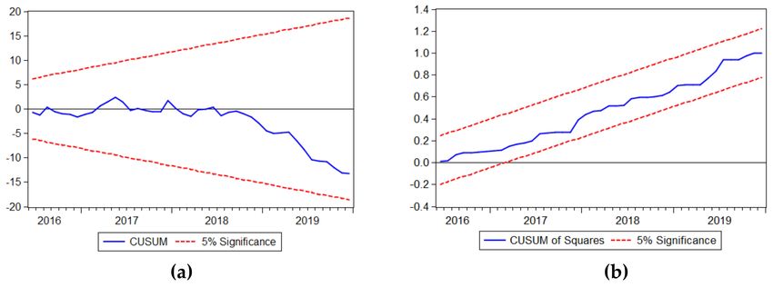
Sustainability 2020, 12, 2798                                                                        2 of 23

rates on economic growth by relating domestic growth to the external business climate, measured by
means of business climate indicators.
      The main goal of the National Bank of Romania (NBR) is to ensure and maintain price stability
and its main tasks are to design and implement the monetary policy and the exchange rate policy.
The monetary policy interest rates influence the short-term money market levels of interest rates, which,
in their turn, can stimulate investment, consumption or saving. In line with Keynesian argumentation,
interest rate reduction may stimulate the aggregate demand in the short run, being at the same time an
impulse to increase investments. Such a measure may have beneficial effects for immediate economic
growth, but it discourages savings. The threat of inflation and the inability to sustain both high
consumption and increased investments mean that, in the long run, we should expect distortions in
the relative price system and a faulty resource allocation (as the Austrian business cycle theory shows).
A low interest rate also leads to a decrease in foreign direct investment (FDI) attractiveness, resulting
in lower capital flows and currency depreciation. Low interest rates could stimulate economic activity
in the short term, but it could distort the relative prices and cause malinvestments. The appreciation of
a currency will lead to cheaper imports and could cause lower inflation. It may lift the standard of
living as people could afford buying more goods. The effects of an appreciation depend on the price
elasticity of demand for imported and exported goods, the phase of the business cycle, if domestic
economy is in an expansionary or a recessionary phase and on the economic context of the trading
partners. In the short run, it is depreciation that could drive economic growth through cheaper
exports (that is why so many developing countries prefer to depreciate their currency, even with
the risk of inflation), but an appreciation, if it is the result of improved competitiveness, does not
exclude economic growth. The alignment of Romania’s interest rate with the interest rate of the Euro
area, and the equilibrium between the monetary policy and exchange rate policy, provide clues for
taking into consideration the European business climate in the decisions made on domestic policies.
The economy trends in the Euro area are emphasized by the GDP evolution, while its changes can
be predicted by consumer and business confidence indicators. The relationship between confidence
and cyclical fluctuations of the economic activity has been debated since the 1920s. Barsky and Sims
identified two distinct perspectives regarding the role of confidence in macroeconomics [1]. One
perspective supports the effect of autonomous changes in the consumers’ behaviour on the economic
activity. Thus, the optimistic or pessimistic waves, labelled as “animal spirits”, are considered major
determinants of economic fluctuations, following A. Pigou and J.M. Keynes. The second perspective
identifies fundamental information about the current and future state of the economy in measuring
the indicators of consumers’ behaviour. The confidence factors, reflected in the Business Confidence
Indicator, provide important information about the business climate in the Euro area, being strongly
linked to the economic growth.
      To reach our goal, we set the following objectives: (i) To analyse the evolution of the economic
growth rate in comparison with the monetary policy interest rate, the exchange rate and the business
climate in the Euro area; (ii) to identify the structural breaks occurred in the evolution of the considered
variables; (iii) to measure the impact of these variables on the economic growth in Romania.
      The results of this study show that in Romania, the monetary policy interest rate, the real exchange
rate and the European business climate have significant influences on the economic growth. The impact
of these factors on the economic growth was measured using the ARDL model, corrected with the
dummy variables attached to the structural breaks.
      The paper has five sections. After the introductory section, Section 2 presents the general
framework of the literature on the relationship between economic growth, interest rate, exchange rate
and business climate, and describes the research hypotheses. Section 3 comprises the description of the
data and used methodology. The results are presented in Section 4. The paper ends with discussions
and conclusions in Section 5.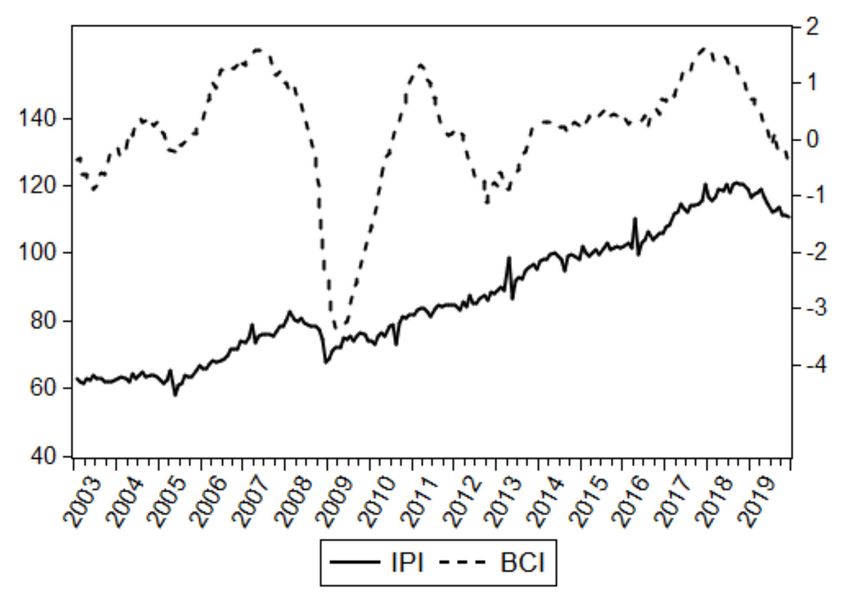
Sustainability 2020, 12, 2798                                                                       3 of 23

2. Literature Review and Research Hypotheses
      In terms of the relationship between the interest rate and economic growth, such theories as those
put forward by Barro and Sala-i-Martin [2] and Harvey [3] emphasize the impact of interest rate on the
economic growth both in the short and long run. In the context of the short-run economic growth, the
increase in interest rates make the population avoid getting bank loans or investing, these determining
a lower economic activity and, implicitly, a lower level of economic growth.
      The empirical tests of the relations between interest rate and economic growth have been mostly in
favour of their negative relation. Authors such as Hossain [4], Low and Chan [5], Abdelkafi [6] and Ozer
and Karagol [7] applied various methods specific to time series (Granger causalities, autoregressive
models with distributed lag and error correction models) in order to study the influence of monetary
policy instruments on economic growth. The study conducted by Hossain over a period of 62 years on
the determinants of economic growth in Bangladesh indicated that inflation causes an increase in the
interest rate and exchange rate volatility, the latter affecting economic performance [4]. The results
of Low and Chan [5] from a study covering Malaysia are in concordance with the results reported
by Hossain [4], where the inflation rate plays an important role and indirectly influences economic
growth through its effects on the interest rate and exchange rate. Próchniak and Witkowski analysed
the impact of the monetary policy interest rate on the economic growth in EU27 countries during
1993–2010, and in the EU15 between 1972 and 2010, obtaining mixed and unstable results [8]. Thus, for
the years 1993–2004, they found a negative relationship between the interest rate and the economic
growth, but for the years 2005–2010, the estimated coefficient on the interest rate was positive,
questioning the effectiveness of manipulating the interest rate to stimulate the recovery of an economy
in recession. Mallick and Sousa found that contractionary monetary policy (an increase in interest
rate) has a strong and negative effect on the output of Brazil, Russia, India, China and South Africa [9].
Murgia [10] estimated the effects of the interest rate, along with other European central bank monetary
policy instruments, on the industrial production in the Euro area, obtaining the result that industrial
production responds to a monetary policy shock with a decline of over 0.5%. Warman and Thirlwall
found no favourable effects of interest rates on economic growth in Mexico between 1960 and 1990 [11].
      Analysing the transmission mechanism of monetary policy for 10 transition economies during the
years 1995–2002, Ganev et al. found that a positive interest rate shock reduced output in the short run
in Slovakia, Hungary and Slovenia, raised it in Lithuania, Estonia, Czech Republic and Poland, but
had mixed results for Latvia, Bulgaria and Romania [12]. At the same time, Ozer and Karagol showed
that the relation between the monetary policy interest rate and economic growth is significant only in
the short run [7].
      Other economic theories show a bidirectional relationship between the interest rate and economic
growth. On the one hand, economic growth can influence the interest rate [13–17] while, on the
other hand, the interest rate may influence the economic growth [18–20]. Abdelkafi highlighted that
there is a bidirectional relation between them, the monetary policies and the economic activity being
interdependent [6]. Lee and Werner rejected the canonical theory of the influences that the interest
rate may have on economic growth, obtaining for the United States, Germany, UK and Japan reversed
Granger causalities and stating that economic growth is a cause factor for the interest rate [21]. Thus,
they believe that the interest rates, both in a short and long run, follow the nominal GDP trend.
      As far as the influence of the exchange rate on the economic growth, two main channels have
been identified: international trade and investments.
      The positive relation between international trade and economic growth can be found in the
literature since that of Adam Smith. The works of the last decades have especially analysed the
empirical evidence of the impact of trade on growth with mixed results according to the analytical
instruments and used assumptions. The dogmatic approach, rooted in the economic logic, is found in
the OECD report regarding the sources of economic growth. Therefore, international trade is not only
linked to the benefits resulting from the exploitation of comparative advantages, but it also provides
additional gains in terms of economic growth by means of scale economies, competition exposure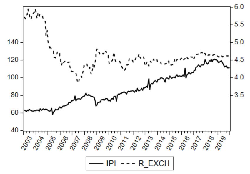
Sustainability 2020, 12, 2798                                                                        4 of 23

and knowledge transmission [22]. Similarly, the study conducted by Frankel and Romer concluded
that trade increases income by stimulating the accumulation of capital [19]. Irwin and Tervio, when
analysing the relationship between international trade and economic growth throughout the 20th
century, reached the same conclusion: Countries with a higher proportion of international trade in
their GDP have higher incomes [23].
      If international trade positively influences economic growth, exchange rate has a significant role
in trade flows. A UNCTAD study of 2013 reports that exchange rate misalignments substantially affect
international trade, being responsible for trade diversion, quantifiable at approximately one percent
of the global trade [24]. The examination, in an IMF study, of historical evidence of the relationships
between exchange rate, prices and volume of international trade for 60 economies reached the following
result: Exchange rate movements tend to have strong effects on exports and imports. The study
estimates that a depreciation by 10 percent of a domestic currency is associated, on average, with 1.5%
of GDP rise in real net exports [25].
      Investments are another important source for domestic and foreign economic growth. Investments
can stimulate economic growth by diffusing knowledge, being an important source of know-how and
human capital. The relationship between investments and growth is a bidirectional one. Iamsiraroj
identified a virtuous cycle that “suggests that FDI contributes to economic growth and growth attracts
FDI inflows, which in turn stimulates growth further” [26]. Foreign direct investments have an
important contribution to economic growth by means of technology transfer, especially in economies
with a significant absorption capacity [27].
      As far as the relationship between exchange rate and economic growth is concerned, S, ipos, and
Boleant, u proved the existence of a unidirectional relation between them, the exchange rate having
a decisive impact on economic growth in Romania [28]. At the opposite end, Anaripour indicated
that in the case of specific countries in South America and Asia, there is a reversed causality between
the two variables, the economic growth having a significant effect on the exchange rate [29]. Rodrik
showed that a high real exchange rate stimulates economic growth [30]. On the same line, Razmi et al.
identified a positive relation between the real exchange rate undervaluation and economic growth,
especially in the case of emerging economies [31]. Ribeiro et al. claimed that the real exchange rate
affects growth indirectly through its impacts on functional income distribution and technological
innovation [32].
      Using a VAR model, Wesseh and Lin found that the depreciation of the Liberian dollar causes a
decrease in the real GDP, while its appreciation has no impact on real GDP in Liberia [33]. Habib et al.
used data for 150 countries for the period 1970–2010 and found that a real appreciation significantly
reduces the annual real GDP growth [34]. Eichengreen asserted that the maintenance of the real
exchange rate at a competitive level and the avoidance of excessive volatility are important for economic
growth [35]. On the other hand, Ihnatov and Capraru claimed that, even if the exchange rate stability
is important for ensuring economic growth, it loses its function when the obtained stability involves
important interventions of the monetary authorities [36].
      An important role in attracting investments is played by the business climate in the destination
country. Thus, price stability, exchange rate predictability and economic stability of a country
determine the increase in interest and confidence of investors to start up a business in a foreign country.
The changes in the exchange rate generate responses in the FDI inflows. Oliveira found that the greater
the volatility of the exchange rate, the lower the investments [37]. Sharifi-Renani and Mirfatah reached
the same conclusion, the exchange rate volatility, by increasing risk and uncertainty, reduces FDI
incentives [38]. Froot and Stein examined the relationship between exchange rate and investments
and showed that the changes of exchange rate determine changes in wealth, which in turn generates
modifications in the demand of direct investments [39]. When analysing the FDI determinants in
the United States, Grosse and Trevino concluded that an appreciation of the exchange rate and an
increase in the purchasing power for American assets lead to an increase in foreign investments in
that country [40]. For US economy, Klein and Rosengren’s study also stated that “a depreciation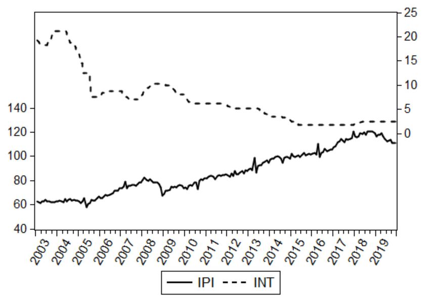
Sustainability 2020, 12, 2798                                                                        5 of 23

(appreciation) of the bilateral real exchange rate is correlated with an increase (decrease) in the inflow
of FDI” [41]. Takagi and Shi found that Japanese FDI in the Asian economies declined with the yen
depreciation against the currencies of the host countries [42].
      In a less conventional way, but no less relevant, economic growth can be estimated based on the
confidence indicators. These confidence indicators could be estimated at the national or regional level.
For our study we referred to the Euro area confidence indicator. The consumers’ confidence and the
climate of confidence where different producers from different industries perform their activity, are
useful indicators which allow to keep track of the economic evolution in the Euro area [43]. The use of
confidence indicators has its origin in an approach started in the 1940s at the University of Michigan.
Katona’s Index of Consumer Sentiment (1951) lays the foundations of using consumer behaviour in
the estimation of the dynamics of consumption expenditures in the United States. At the European
level, the confidence indicators target both the consumers and the producers (grouped by activity
sectors: industry, constructions, retail trade and services). Analysis of the Euro area’s economic activity
is facilitated by the use of composite indicators, which, through their monthly frequency, allow for
a better monitoring of the economic activity [44]. Strigel showed there is a very good relationship
between economic climate indicators and economic performance, these providing early indices on
the direction of the cyclical evolution of the economy [45]. Furthermore, the climate indicators reflect
quite quickly the changes in financial variables (the interest rate, the exchange rate) that affect the
“sentiment” of consumers and producers [45]. Thus, the confidence/sentiment indicators can function
as “early barometers” in the evolution of an economy [46].
      Measuring the business sentiment provides valuable information for the evaluation of the
economic situation and for performing forecasts as shown by the OECD study performed by Santero
and Westerlund [47]. They examined the relationship between consumer and business confidence
indicators and the GDP for 11 OECD countries for the period 1979–1995. The relevance of the confidence
indicators also comes, according to the authors, from the fact that the data obtained in qualitative
surveys (sentiment data) are more relevant because the trend and seasonality issues are avoided, being
at the same time isolated from the distortions that may characterize ”real” statistics. Data lags and
data revisions lengthen the measuring processes, while the confidence indicators track the major
cyclical movements of industrial production. If Santero and Westerlund identified a limit in the use of
confidence indicators for the performance of short-run forecasts, due to lack of a sequential behaviour
consistent with the movements in the production activity, Mourougane and Roma considered that
these can be useful in forecasting the growth rates of GDP [48]. Using a Dynamic Factor Model (DFM),
Hansson and Jansson showed that, for Sweden, the data from the business tendency surveys are useful
for forecasting the short-run GDP evolution [49].
      Demirel and Artan studied the effects of confidence indicators on the macroeconomic variables
in 13 European Union countries for the period 2000–2014 and showed that confidence influences the
production level, the consumption level, inflation rate and unemployment [50]. Furthermore, trust is
associated with better economic performances, as stated by Knack and Keefer [51], while Gennaioli
found that expectations have a major role on economic growth [52]. In the study of Das and Das [53]
the Business Confidence Indicator (BCI) is a significant variable for economic growth in Germany,
Spain and Japan. Alves [54] found that fluctuation in the Business Confidence Indicator (BCI) have a
significant impact on Portugal’s industrial production. Zanin analysed the relationship between the
changes in the Economic Sentiment Indicator and the GDP increase for six countries, with mixed results.
The best relations were obtained for France and Italy, included in the group of the most developed
economies in the Euro area [55]. Using an autoregressive distributed lag (ARDL) model for South
Africa, De Jongh and Mncayi found that an increase of one percent in business confidence may lead to
an economic growth of 0.23% [56].
      The traditional perspective to measuring economic activity is based on information provided by
the GDP indicator. Beyond its measuring limits, GDP provides only quarterly or annual information.
Moreover, the gap of several weeks between the data publication and the period they refer leads to
Sustainability 2020, 12, 2798 6 of 23
belated knowledge about the evolution of a country’s economy. Although important, it would be more
helpful to use information with higher frequencies, such as monthly data. Therefore, we will use the
Industrial Production Index (IPI) to measure economic growth.
The analysis of the relationship between the interest rate, the exchange rate and the economic
growth in Romania is the main goal of our study, to which we will also add the influence of the business
climate in the Euro area.
Using the main lines of research identified in the literature review, we formulated the following
research hypotheses:
Hypothesis 1. The interest rate influences economic growth in Romania.
Although the Central Bank of Romania does not aim to stimulate economic growth, the
establishment of market policy interest rate for open market operations provides a significant sign of
access to consumption and investment loans. This way, the interest rate calibrates both supply and
demand in economy, being a determining factor of growth.
Hypothesis 2. The exchange rate influences economic growth in Romania.
Managed float regime allows the Central Bank of Romania to respond in case of external shocks,
at the same time, the exchange rate influencing the economic activity through net exports and wealth
and balance sheet effects. Stimulation of exports and industrial production by means of monetary
depreciation should be put in balance with inflation, indebtedness and capital flights.
Hypothesis 3. The business climate in the Euro area influences economic growth in Romania.
Business climate measures the trust of producers in positive evolution of economy. Growth of
demand and economic activity in the Euro area are incentives for industrial production in Romania,
being heavily dependent on the European market.
3. Data and Empirical Methodology
3.1. Data
This study analyses the data regarding the industrial production index, the monetary policy
interest rate, the real exchange rate and the Euro area Business Climate Indicator for the period
January 2003–December 2019. In order to eliminate the influence of seasonal variations, we took into
consideration the seasonally adjusted variant of the industrial production index and the Euro area
Business Climate Indicator. The data were collected from the websites Eurostat and the National Bank
of Romania.
The industrial production index (IPI) is calculated as a Laspeyres index and measures the changes
in the production volume at regular intervals, usually every month [57]. IPI is one of the most relevant
indicators for measuring real economy, and in this study it is used as a measure of economic growth.
In Romania, for the analysed period, which also comprises the economic/financial crisis of 2007 that
extended until 2010–2012, some branches of the national economy, such as agriculture and construction,
went through an accentuated decline. Industry continued to be the main pillar of economic growth
and, even if during the privatization process it had suffered a lot, it maintained its major contribution to
the GDP, comprised between its lowest level, equal to 23.1% registered in the years 2015 and 2016 [58],
and its highest level of 26.4% in 2010 [59].
Taking into account that industrial production holds the dominant weight in the total economic
activity, when highlighting the changes in the industrial production volume, the industrial production
index provides a general overview of the dynamics of a country’s economy. The monthly data of the
industrial production index provides businesses with information on the production changes, andSustainability 2020, 12, 2798 7 of 23
indirectly, on the changes of domestic economic growth. At the same time, political decision-makers
can use the data of the industrial production index as signals in handling monetary or fiscal policy
instruments. The set of instruments used by the National Bank of Romania (NBR) to implement
its monetary policy count open market operations, standing facilities and reserve requirements.
The monetary policy interest rate is the interest rate used for the main open market operations of the
NBR. Currently, these are one-week repo operations. Monetary policy rate replaces the NBR’s reference
interest rate starting with the 1st of September 2011 [60].
The exchange rate represents the price based on which a currency is changed with another one,
namely, the ratio between a domestic currency and a foreign one. The real exchange rate is of great
importance for both decision makers and economic agents because it reflects the competitiveness of
prices and costs [61]. The real exchange rate is determined by adjusting the nominal exchange rate to
the inflation rates between the two countries, according to the relation
HICP_i
R_EXCH = N _EXCH (1)
HICP_RO
where R_EXCH is the real exchange rate, N_EXCH is the nominal exchange rate and HICP_RO and
HICP_i is the consumer price indices in the country, respectively, out of the country.
For the calculation of the RON/Euro real exchange rate, the authors used the consumer price index
for Romania and, respectively, the average consumer price index for the Euro area. The interest rate
and the exchange rate do not have seasonal variations and their seasonally adjustment was not needed.
The Euro area Business Climate Indicator (BCI) is a composed indicator of the manufacturing
industry in the Euro area and it is obtained by processing the data collected through business and
consumer surveys. These surveys are performed on a monthly basis by the Institute of Statistics of the
member states or of the states in the process of adherence to the European Union and, respectively, of the
member states of the Organisation for Economic Cooperation and Development (OECD). The business
and consumer surveys are performed in the following sectors of economic activity: manufacturing
industry, construction, consumption, retail trade and services. An important feature of the business and
consumer surveys is that almost all the questions are qualitative. The goal of business and consumer
surveys is to calculate confidence indicators in order to reflect the evolution of the macroeconomic
indicators, being the key complement of official statistical data, which in general are quantitative.
BCI is computed based on the answers provided by the representatives of the biggest companies in
the manufacturing industry in the Euro area to five questions regarding production trends in recent
months, order books, export order books, stocks and production expectations [43]. The method used
to determine BCI has at its basis the fundamental principles of the Principal Component Analysis
(PCA) and it is represented by the main factors extracted from the five components of the industry
survey. Calculated in this manner, it is believed that BCI must increase alongside the entire industrial
activity in the Euro area and the BCI importance is supported by the fact that more than a half of the
GDP variations are represented by the fluctuations of the industrial activities [44]. For that matter, the
European Commission considers the economic climate as being of utmost importance in the evolution
of an economic cycle while the confidence indicators in an industry have the advantage that they offer
a lot more and quicker information about the GDP evolution than the official statistical data [62].
In this paper, the authors used the following symbols for the variables: the industrial production
index—IPI; monetary policy interest rate—INT; the real exchange rate—R_EXCH; and the Euro area
Business Climate Indicator—BCI.
3.2. Empirical Methodology
In order to empirically analyse the long-run relationships and the short-run dynamic interactions
among the variables, we applied the autoregressive distributed lag (ARDL) cointegration technique.
The research approach comprises the following steps: (1) testing for the unit root without and withSustainability 2020, 12, 2798 8 of 23
structural breaks for the selected variables; (2) identifying the types of relationships among the variables;
and (3) modelling the relationships among variables.
3.2.1. Testing for Unit Roots and Structural Breaks
Since the ARDL approach cannot be applied when some variables are integrated with a two
or higher order than two, it is important to perform unit root tests on all regressors [63]. There are
several unit root and stationarity tests, such as Augmented Dickey–Fuller (ADF) [64], Phillips–Perron
(PP) [65], Kwiatkowsky–Phillips–Schmidt–Shin (KPSS) [66] or Dickey–Fuller Generalized Least Squares
(DF-GLS) [67]. However, these tests do not account for the potential structural breaks in the time
series and could provide spurious results when the data are trend stationary with a structural break.
The unit roots tests with structural breaks evolved from Perron [68] (considering one known structural
change) to Zivot and Andrew [69] (considering one unknown break) and Lumsdaine and Papell [70]
(considering two unknown breaks). Lee and Strazicich point out that the main drawback of the ZA
and LP tests is that they assume breaks only under the alternative hypothesis [71]. Carrion-I-Silvestre
et al. [72] propose robust versions for the tests originally developed by Ng and Perron [73], which
allow for multiple structural breaks under both the null and the alternative hypotheses. The previous
authors suggest implementing a pretesting procedure to assess whether a series has structural change
in level and / or slope [74].
The Perron and Yabu [75] procedure checks for the presence of structural change, without prior
knowledge of the series’ order of integration. If a structural change is found, the robust unit root tests
of Carrion-I-Silvestre et al. [72] are employed. If no breaks occur, unit root tests, such as the Augmented
Dickey–Fuller and the Phillips–Perron can be used.
The Perron and Yabu procedure [75] considered three types of structural change: (i) Model
I—structural change in the intercept; (ii) Model II—structural change in the slope; and (iii) Model
III—structural change in the intercept and in the slope. The Perron and Yabu statistic test, called
Exp-WFS, is based on a quasi-feasible Generalized Least Squares approach, using an autoregression
for the noise component with a truncation to 1 when the sum of the autoregressive coefficients is in the
neighbourhood of 1, along with a bias correction. According to Oscar Bajo-Rubio [76], for given break
dates, Perron and Yabu [75] propose an F-test for the null hypothesis of no structural change in the
deterministic components using the Exp function developed by Andrews and Ploberger [77].
The second step of the stationarity analysis consists of applying the Carrion-I-Silvestre et al. [72]
set of robust tests to the series that feature a break in the trend function. Carrion-I-Silvestre et al.
generated five different test statistics to check for the null hypothesis of a unit root under multiple
structural breaks, which are the Elliot et al. [67] feasible point optimal test (PT GLS ) and its modified
version (MPT GLS ), the Phillips [78] modified test (MZα GLS ), the modified Sargan and Bhargava [79]
test (MSBGLS ) and the modified Phillips and Perron [65] test (MZtGLS ). The superscript GLS indicates
that all the series are GLS detrended [74]. These tests are applied on the following models: (i) Model
1—for the constant case, without structural breaks; (ii) Model 2—for the linear time trend case, without
structural breaks; (iii) Model 3—for the linear time trend with multiple structural breaks, which affects
both the level and the slope of the time [80]. For all tests, the null hypothesis is rejected if the test
statistic is smaller than the relevant critical value, suggesting the absence of a unit root in the series.
3.2.2. The ARDL Bound Cointegration Test
Even if the Autoregressive Distributed Lag (ARDL) models have been used in econometric
modelling for decades, they have only gained popularity in recent years when they were used in the
methods analysing cointegration relationships. In this regard, important contributions were made
by Pesaran and Shin [81] and Pesaran, Shin and Smith [82]. Unlike other existing methods in the
literature, such as Engle–Granger [83] and Johansen–Juselius [84], the ARDL cointegration method has
the advantage to verify the existence of long-term relationships between variables that have different
orders of integration, while the results of the analysis are robust for an incorrect specification of theSustainability 2020, 12, 2798 9 of 23
order of integration. Other advantages of the ARDL cointegration technique mention the following
aspects: Different restrictions can be applied in terms of the optimum number of lags of the variables
under consideration [85]; it is based on a single equation, which estimates simultaneously both the
short-run and the long-run relationships, which makes it easy to implement and interpret [86–89].
The ARDL Bound test model, used in this study is expressed as follows [90,91]:
p−1
X k qX
X j −1 k
X
∆Yt = βi ∆Yt−i + δ j,l j ∆X j, t−l j + θYt−1 + φ j X j, t−1 + λzt + ut (2)
i=1 j=1 l j =0 j=1
where Yt is the dependent variable from the ARDL model, IPI in this study; X j,t , j = 1, k is the
independent variables, INT, R_EXCH and BCI in this study; k—the number of independent variables; zt
is an s x 1 vector of deterministic variables such as the intercept term, dummy variables or time trends;
ut —the error term, βi and δ j,l j are the coefficients of the terms that indicate the short-run relationships;
θ and φ j are the coefficients of the terms that indicate the long-run relationships; p and q j represent
optimal lags for the variables Yt and X j,t identified based on information criteria; and λ represents the
coefficient attached to a term of the vector zt .
The bounds test consists of testing the null hypothesis of no cointegration or long-run relationship
between the considered variables using Fisher statistics. The null hypothesis is formulated regarding the
coefficients from Equation (2) as follows: H0 : θ = 0, φ j = 0, ∀ j = 1, k. The asymptotic distribution
of the test statistic is non-standard and Pesaran et al. [81] calculated the critical values for F-statistics.
These critical values are obtained for different circumstances and define an interval for which the lower
bound is determined based on the hypothesis that all variables are I(0), while the upper bound is
calculated based on the hypothesis that all variables are I(1). The critical values of Pesaran et al. [82]
are only useful and efficient for large sample sizes. Kripfganz and Schneider [92] extended the work
of [82], determining with stochastic simulations the critical values that cover a full range of possible
sample sizes and lag orders, allowing any number of variables in the long-run-level relationship.
According to the decision rule, if the calculated value of the F statistic is higher than the upper
bound, the variables are cointegrated, and if it is inferior to the lower bound, then all variables are I(0),
which means no long-run relationships can exist—in other words, the cointegration test is inconclusive.
The testing is completed by the verification of the significance of coefficient θ corresponding to
the term Yt−1 , using the t test. As in the case of F-statistics, the asymptotic distribution of the t test
statistics is non-standard, and the critical values of the t-statistics are provided by Pesaran et al. [82].
The absolute values of the t-statistics are compared against the corresponding critical values and the
decision rule is similar to the one presented above for the Fisher test.
3.2.3. Modelling the Relationships between the Variables
According to the cointegration test results, for the modelling of the relationships between variables,
different types of models are applied. If between the variables under consideration there are long-run
relationships, an error correction model (ECM) is applied. At the opposite end, if there are no long-run
relationships between variables, a short-run ARDL model is applied [81]. To validate the previously
estimated model, the short-run ARDL or ECM, it is necessary to verify the hypotheses for the model
coefficients and residual component.
The stability of coefficients is verified, according to the authors Brown et al. [93] and Pesaran
and Pesaran [94], through the graphical representation of the cumulative sum of recursive residuals
(CUSUM) and, respectively, the cumulative sum of square recursive residuals (CUSUM of Squares).
The coefficients are stable if, within the two representations, the variance of residuals fits within the
interval that indicates the variation limits for a significance level at 5%. In order to verify if the model
should be linear, it can be formally tested using Ramsey’s RESET test [95], which is a general test forSustainability 2020, 12, 2798 10 of 23
misspecification of functional form. If the value of the test statistic is greater than the χ2 critical value,
the null hypothesis of the correctness of the functional form is rejected [96].
For validation of the model, it is also necessary to check the hypotheses formulated on the residual
component using tests such as Jarque–Bera for the normality hypothesis; the Breusch–Godfrey Serial
Correlation LM test for no serial correlation; as well as the Breusch–Pagan–Godfrey and ARCH tests
for homoscedasticity.
The model robustness can be verified by comparing the results obtained through the ARDL
approach with those indicated by the causality analysis, performed through the Granger causality
test or the Toda–Yamamoto approach. The significance tests of the short-run or long-run coefficients
and the Granger causality tests can identify causality relationships between variables in at least one
direction [97,98].
4. Results
4.1. A Comparative Analysis of Economic Growth vs. The Interest Rate, the Exchange Rate and the European
Business Climate Evolution
In this section, we analyse the evolution of economic growth, measured by the industrial production
index, in comparison with the evolution of the monetary policy interest rate, the real exchange rate
and the Euro area Business Climate Indicator. The comparison of these evolutions focuses on the
identification of the correlations between the industrial production index and the influence factors
under consideration.
The comparative analysis of the industrial production index and the monetary policy interest
rate evolution in Romania between January 2003 and December 2019, is shown in Figure 1. It can
be observed that the two indices have a different evolution during January 2003 and March 2018,
ascending in the case of the industrial production index and descending in the case of the monetary
policy interest rate.
Figure 1. The evolution of the industrial production index and of the monetary policy interest rate
in Romania.
Monetary policy interest rates have decreased significantly since 2003, when they reached 20%,
to values below 2% in 2015. In the context of Romania’s adherence to the Euro area, the decrease in the
monetary policy interest rate, as a result of the efforts to align the interest rate in Romania with the
monetary policy in the Euro area, had a positive effect on industrial production. It can also be observed
that the level of the interest rate during the period 2014–2019 is almost constant, with small decreases
during the period 2015–2017, confirming the trend toward meeting a real sustainable convergence.
Based on the graphical analysis, a negative relation between the two variables is observed.
In terms of comparative analysis of the evolution of the industrial production index and the
real exchange rate in Romania (Figure 2), it can be seen that for a great part of the analysed period
both indices have tendencies of slight increase. The outbreak of the economic crisis determined the
beginning of the real exchange rate growth tendency in Romania. The inflationist pressures andSustainability 2020, 12, 2798 11 of 23
the obvious break between savings, consumption and investments (see the Austrian theory of the
economic cycle) imposed the increase in the interest rate. This way, the monetary policy in Romania
followed the evolution of the Euro area, having as a goal the slight increase of the real exchange
rate in order to reach a level close to the nominal convergence criterion for the fluctuation interval
established according to the European Mechanism of Exchange Rates. In 2008 and 2009, more severe
depreciations of the nominal RON/EUR exchange rate occurred due to tensions on the international
markets, increasing mistrust of foreign investors, risk aversion and lower volume of liquidities [99].
After 2010, the industrial production and the real exchange rate have had similar trends, indicating a
positive relationship between them.
Figure 2. The evolution of the industrial production index and of the real exchange rate in Romania.
The comparative analysis between the industrial production index evolution in Romania and
the Euro area Business Climate Indicator (Figure 3) shows that the two indices have a similar trend:
During the period January 2003–December 2007, there was an increasing trend in the values for
the two indices; at the beginning of the year 2008 there was a significant decreasing trend for both
indices, these returning at approximately equal values within a 3-month interval; during the period
January 2011–March 2018, there was a tendency of a slight increase in the values of both indices,
with weak fluctuations; and during the period April 2018–December 2019, both indices had a slight
decreasing tendency.
Figure 3. The evolution of the industrial production index in Romania and of the Euro area Business
Climate Indicator.
The significant decreases in the values of the two indices, signalled at the beginning of 2008, are
due to the effects of the global economic crisis at the end of 2007. So, economic activities in all economic
sectors in Romania were negatively affected, especially the industrial sector that contributes the most to
the GDP formation of Romania. The price instability in the industrial sector determined a decrease in
investors’ confidence in the Romanian market and, implicitly, their withdrawal, which created effects
such as the contraction of industrial production and an increase in the unemployment rate. As far as theSustainability 2020, 12, 2798 12 of 23
Euro Area Business Climate Indicator are concerned, they had a decrease of approximately 4% against
the normal values. The effects of the economy manifested more intensely in Europe, while confidence
in the economy decreased significantly. Within a 3-year interval, the negative effects of the crisis
decreased, and the Euro area Business Climate Indicator reached values similar to the pre-crisis period.
4.2. Testing for Unit Roots and Structural Breaks of the Variables Considered
The first step of the approach of most modelling analyses of time series is to verify the stationarity
of the variables analysed. The preliminary graphical analysis indicated some structural breaks,
explained by the events that occurred in the analysed period, such as the economic and financial crisis
of 2008. Furthermore, IPI, INT and R_EXCH present a linear trend, while BCI does not. In this regard,
for the first three mentioned variables, the pre-test developed by Perron and Yabu [75] was performed
in order to assess whether a structural break is present in the deterministic components.
The results of Perron and Yabu’s test are presented in Table 1. According to the obtained results,
the null hypothesis of an absence of a structural break in the intercept and slope is rejected at the 1%
level of statistical significance for all three considered variables. The last column of the table includes
the identified structural breaks.
Table 1. Results of the Perron and Yabu test.
Variables Test Statistic Break
IPI 6.319 *** 2008M10
INT 95.702 *** 2005M06
R_EXCH 49.134 *** 2007M10
Note: *** denotes significance at the 1% level.
Afterwards, we analysed the order of integration of the variables IPI, INT and R_EXCH, taking
into consideration the presence of structural breaks. In this respect, the quasi-GLS approach of Carrion
et al. [72] was applied, including the following set of unit root tests: PT GLS , MPT GLS , MZα GLS , MSBGLS
and MZt GLS . These tests were performed for each of the variables in levels and in 1st difference.
The results are summarized in Table 2.
Table 2. Results of the Carrion et al. unit root tests.
Variables PT GLS MPT GLS MZα GLS MSBGLS MZt GLS Breaks
Levels a
IPI 19.300 18.531 −10.415 0.208 −2.171 2013M03, 2013M05, 2016M04
INT 7.437 7.377 −18.582 0.161 −2.994 2004M05, 2005M03, 2005M07
R_EXCH 8.970 8.504 −23.187 0.146 −3.404 2004M10, 2004M12, 2008M08
1st difference b
IPI 1.073 ** 1.072 ** −85.512 ** 0.076 ** −6.537 ** -
INT 4.095 ** 4.132 ** −22.061** 0.150 ** −3.320 ** -
R_EXCH 1.378 ** 1.387 ** −65.888 ** 0.087 ** −5.738 ** -
Notes: ** denotes significance at the 5% level. a A model with structural breaks that affect both the level and the
slope of the time trend was applied. b A model with a trend, without structural breaks was estimated. The lag
length for all the tests is selected via the MAIC criterion suggested by Ng and Perron [72].
For all tests, the null hypothesis is rejected if the test statistic is smaller than the relevant critical
value. As it can be seen from the results above for IPI, INT and R_EXCH in levels, the null hypothesis is
not rejected at the 5% level of significance. Table 2 also shows for each considered variable a maximum
of three structural breaks that occurred in their evolution during the period January 2003–December
2019. For the variables in 1st difference, the unit root tests indicated the absence of a unit root,
meaning that the considered variables have a maximum of one order of integration in the presence of
structural breaks.Sustainability 2020, 12, 2798 13 of 23
Regarding BCI, the results of the Augmented Dickey–Fuller (ADF) and Phillip–Perron (PP) unit
root tests, presented in Table 3, revealed that it is stationary at level.
Table 3. Results of the Augmented Dickey–Fuller (ADF) and the Phillip–Perron (PP) unit root tests.
ADF a PP a
Variable t-Test t-Test Order of t-Test t-Test Order of
(Level) (1st Difference) Integration (Level) (1st Difference) Integration
−4.577
BCI - I(0) −2.568 ** - I(0)
***
Notes: a Model with intercept and trend. *** and ** denote statistical significance at the 1% and 5% level, respectively.
Overall, the unit root tests indicate that the variables are integrated in the mixed order, but none
are integrated for order two. These results determined a favourable context to the application of an
ARDL Bounds test for cointegration.
4.3. The ARDL Bound Cointegration Test
In order to estimate the ARDL model, we performed a VAR model to identify the optimal number
of lags between variables. Based on the results of the information criteria FPE, AIC, SC and HQ, we
selected a number of five lags.
The validation of the ARDL model based on which the Bound test is applied implies the verification
of coefficient stability and of hypotheses concerning the error variables. The representation of the
CUSUM of Squares indicates the instability of coefficients for the ARDL model. For the model
correction, dummy variables, as exogenous elements, were introduced, which were defined in relation
to the structural breaks that determine the coefficients instability: a step dummy variable for the
structural break identified in IPI (2008M10) by the Perron and Yabu test and some impulse dummies for
the structural breaks identified in IPI (2013M03, 2013M05 and 2016M04) by the Carrion et al. tests [100].
The results of the ARDL Bounds test, regarding the existence of long-run relationships between
IPI and the independent analysed variables, are presented in Table 4. In order to obtain more precise
results for this test and because we have a small sample, we considered both the set of critical values,
as proposed by Pesaran et al. [82] and Kripfganz and Schneider [92].
Table 4. Results of ARDL Bounds Test.
Critical Values
Test Statistic Significance (a) (b)
I(0) I(1) I(0) I(1)
F-statistic
4.775 10% 3.47 4.45 3.408 4.473
5% 4.01 5.07 3.969 5.125
2.5% 4.52 5.62 - -
1% 5.17 6.36 5.193 6.526
t-statistic
−2.327 10% −3.13 −3.84 −3.070 −3.757
5% −3.41 −4.16 −3.396 −4.086
2.5% −3.65 −4.42 - -
1% −3.96 −4.73 −3.952 −4.710
Notes: (a) denotes the critical values proposed by Pesaran et al. [81] and (b) denotes the critical values proposed by
Kripfganz and Schneider [91].
The results showed that the value of F-statistic from the ARDL model is inferior to the critical
values of Pesaran et al. [82] and Kripfganz and Schneider [92] for the lower bound, I(0), for a 1% level
of significance. Regarding the t-statistic, the absolute calculated value is lower than the critical valuesSustainability 2020, 12, 2798 14 of 23
of the lower bound proposed by the previous authors for all the levels of significance considered.
According to the above results, the null hypothesis cannot be rejected, which means that there is
no co-integration among the variables. Therefore, it can be concluded that between IPI and the
other considered variables are only short-run relationships. The modelling of these relationships is
performed using the short-run ARDL model.
4.4. Econometric Model of the Economic Growth in Romania
The short-run ARDL model of IPI in relation to the variables INT, R_EXCH and BCI is presented
in Table 5.
Table 5. Estimates from the autoregressive distribute lag (ARDL) short-run model.
Regressor Coefficient Std. Error Characteristics
D(IPI(−1)) −0.375 *** 0.063 Dependent variable D(IPI)
D(IPI(−2)) −0.158 *** 0.057 Structural breaks dummies Yes
D(INT) −0.684 ** 0.302 Information criteria AIC
D(INT(−1)) 0.283 0.318 ARDL lag order (2, 2, 1, 4)
D(INT(−2)) 0.230 0.298 R-Squared 0.568
D(R_EXCH) 0.334 1.466 Adjusted R-Squared 0.523
D(R_EXCH(−1)) 4.234 *** 1.463 Log likelihood −369.951
D(BCI) 0.907 0.862 F-statistic 12.434
D(BCI(−1)) 2.855 *** 0.875 Prob(F-statistic) 0.000
D(BCI(−2)) 1.258 0.894 Ramsey RESET Test 0.362 a
Breusch–Godfrey Serial
D(BCI(−3)) 0.714 0.862 0.269 a
Correlation LM
D(BCI(−4)) −2.516 *** 0.858 Breusch–Pagan–Godfrey 0.774 a
C 0.383 0.255 ARCH test 1.176 a
@Trend 0.002 0.003 Jarque–Bera 7.932 b
Notes: a The null hypothesis is not rejected at the 5% level of significance. b The null hypothesis is not rejected at the
1% level of significance. *** and ** denote statistical significance at the 1% and 5% level, respectively.
The coefficients of the ARDL short run showed that IPI is significantly and negatively influenced
by its own values with 1 and 2 lags. The current values of INT also have a significant and negative
influence on the IPI formation, while the lagged values have a positive but not a significant influence.
Regarding the relationship between the R_EXCH and IPI, it can be observed that values of IPI are
positive and significantly influenced by the previous values of R_EXCH lagged by 1 period. Finally,
BCI has a significant impact on IPI, positive at 1 lag and negative at 4 lags.
According to the Fisher test, the short-run ARDL model in relation to INT, R_EXCH and BCI
is statistically significant for a risk of 1%. The value of the determination coefficient indicates that
a percentage of 56.8% from the IPI variation is explained through the ARDL model relative to the
monetary policy interest rate, real exchange rate and Euro area Business Climate Indicator.
Model validation is done on the basis of tests concerning the coefficient stability, the correctness
of the model and the hypotheses on residuals: normality, no serial correlation and homoscedasticity.
The representations of CUSUM and CUSUM of Squares indicate the coefficients stability, the
variation of cumulated residuals and of the squares of cumulated residuals being within the limits of
the interval corresponding to the confidence level of 95% (Figure 4). According to the Ramsey RESET
test (Table 5), the null hypothesis is not rejected, therefore the model is correctly specified. Furthermore,
all hypotheses on residual are verified, therefore the model is validated.Sustainability 2020, 12, 2798 15 of 23
Figure 4. Plots for the (a) CUSUM and (b) CUSUM of Squares.
4.5. Robustness of the Cointegration Analysis
Apart from the ARDL model, we are also interested in the dynamic relationship among the
variables. To this end, in this study we generated impulse–response functions (IRFs) based on Vector
Autoregressive (VAR) system. IRFs trace out the responsiveness of the dependent variable to the shocks
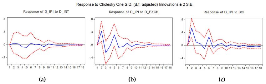
to each of the variables in the system [96]. Figure 5 shows the impulse responses for IPI associated
with separate unit shocks to INT, R_EXCH and BCI considering 18 periods.
Figure 5. Impulse responses of D_IPI for innovations in (a) D_INT, (b) D_EXCH and (c) BCI.
The graph of impulse response function showed that INT indicate a positive effect in Periods 1 to
3 and smooth fluctuations in the following periods, reaching a slight effect in the 10th period. When
the impulse is R_EXCH, the response of IPI has an obvious fluctuation until the steady state beginning
from the 10th period, with the highest positive effect in the 2nd period and a lowest negative effect
in the 3rd period. The impulse of BCI determines, also, an obvious fluctuation in the response of
IPI. The highest positive effect was registered in the 2nd period, while the lowest negative effect was
reached in Periods 5 and 7. The results obtained agrees with the ones from the cointegration analysis,
revealing that impulses to INT, R_EXCH and BCI generate large fluctuations in the response of IPI in
the first 5–6 periods analysed, with smooth fluctuations in the following periods.
To verify the robustness of the results obtained in the previous section, a pairwise Granger
causality test is applied (Table 6).Sustainability 2020, 12, 2798 16 of 23
Table 6. Results of the causality tests.
Null Hypothesis Obs k F-statistic
INT does not Granger cause IPI a 3.364 **
202 2
IPI does not Granger cause INT a 0.052
R_EXCH does not Granger cause IPI a 3.208 **
202 2
IPI does not Granger cause R_EXCH a 1.190
BCI does not Granger cause IPI b 4.939 ***
199 5
IPI does not Granger cause BCI b 1.796
R_EXCH does not Granger cause INT a 2.054
202 2
INT does not Granger cause R_EXCH a 0.012
BCI does not Granger cause INT b 0.455
198 6
INT does not Granger cause BCI b 0.405
BCI does not Granger cause R_EXCH b 1.266
199 5
R_EXCH does not Granger cause BCI b 1.592
Notes: ***, ** and * denote statistical significance at the 1%, 5% and 10% level. a Denotes the causalities between
variables analysed using the Granger causality test. b Denotes the causalities between variables analysed using the
Toda–Yamamoto causality approach.
If both time series are stationary, the causality analysis is performed using the Granger test;
but, if the time series have different integration orders, the causality analysis is conducted using the
Toda–Yamamoto approach [101]. The causality tests confirm the existence of unidirectional causality,
from factors considered in IPI, which means that the monetary policy interest rate, the real exchange
rate and the business climate indicator are Granger cause for IPI (Table 6). The causality relationships
obtained between the considered variables are shown in Figure 6. The Granger causality tests confirm
the cointegration analysis results through the ARDL approach, namely, that INT, R_EXCH and BCI are
cause factors for IPI.
Figure 6. Significant causalities between the Industrial Production Index (IPI) and the considered
factors. Source: Authors’ schema
5. Discussions and Conclusions
The study of economic growth and its determining factors has been the subject of numerous
studies, and due to its importance, it is still a highly relevant topic. Economic growth can be influenced
by a wide range of factors. In this study, we focused on analysing the impact of the interest rate, the
exchange rate and the business climate in the Euro area on the economic growth in Romania, between
January 2003 and July 2019, and in the context of the country’s accession to the Euro area.
The impact of these factors on the industrial production index was analysed using short-run
ARDL models. The main results showed that, in a short run, the two rates have different influences on
the economic growth: The interest rate has a negative influence, while the exchange rate has a positive
influence. These results are consistent with the results described by economic theory and reported by
other empirical analyses.
Our study obtained a reverse relationship between the evolution of interest rate and industrial
production, confirming the capacity of this main instrument of monetary policy to stimulate the
economic activity in the short run. Interest rate reduction decreases the cost of crediting and stimulates
consumption and current supply, encouraging real economy. The risk of inflation rate growth,
distortions in the system of relative prices and a growth in the gap between investments and savingsYou can also read