The MAPM (Mapping Air Pollution eMissions) method for inferring particulate matter emissions maps at city scale from in situ concentration ...
←
→
Page content transcription
If your browser does not render page correctly, please read the page content below
Atmos. Chem. Phys., 21, 14089–14108, 2021
https://doi.org/10.5194/acp-21-14089-2021
© Author(s) 2021. This work is distributed under
the Creative Commons Attribution 4.0 License.

The MAPM (Mapping Air Pollution eMissions) method for
inferring particulate matter emissions maps at city scale
from in situ concentration measurements: description
and demonstration of capability
Brian Nathan1,2 , Stefanie Kremser2 , Sara Mikaloff-Fletcher1 , Greg Bodeker2 , Leroy Bird2 , Ethan Dale2 , Dongqi Lin3 ,
Gustavo Olivares4 , and Elizabeth Somervell4
1 NIWA,  Wellington, New Zealand
2 Bodeker Scientific, Alexandra, New Zealand
3 School of Physical and Chemical Sciences, University of Canterbury, Christchurch, New Zealand
4 NIWA, Auckland, New Zealand

Correspondence: Brian Nathan (dr.brian.nathan@gmail.com)

Received: 21 December 2020 – Discussion started: 27 January 2021
Revised: 16 June 2021 – Accepted: 21 July 2021 – Published: 23 September 2021

Abstract. Mapping Air Pollution eMissions (MAPM) is a 2-         1   Introduction
year project whose goal is to develop a method to infer par-
ticulate matter (PM) emissions maps from in situ PM concen-      The growth of mega-cities from global urbanization has de-
tration measurements. Central to the functionality of MAPM       graded urban air quality sufficiently to impede economic
is an inverse model. The input of the inverse model includes     growth and create a public health hazard (Adams et al.,
a spatially distributed prior emissions estimate and PM mea-     2015). Emissions of particulate matter (PM), photochemi-
surement time series from instruments distributed across the     cally reactive gases, and long-lived greenhouse gases con-
desired domain. In this proof-of-concept study, we describe      tribute to the urban environmental footprint with concomitant
the construction of this inverse model, the mathematics un-      economic and social costs. Recent research has demonstrated
derlying the retrieval of the resultant posterior PM emissions   a link between air pollution levels and elevated suscepti-
maps, the way in which uncertainties are traced through the      bility of the public to pulmonary diseases (Anderson et al.,
MAPM processing chain, and plans for future developments.        2012; Crinnion, 2017). Multiple studies have also character-
To demonstrate the capability of the inverse model devel-        ized increases in hospitalizations for cardiac and respiratory
oped for MAPM, we use the PM2.5 measurements obtained            diseases that are directly correlated with increases in PM2.5
during a dedicated winter field campaign in Christchurch,        concentrations (e.g. Dominici et al., 2006; Zanobetti et al.,
New Zealand, in 2019 to infer PM2.5 emissions maps on a          2009). With regard to the recent COVID-19 pandemic, Zhu
city scale. The results indicate a systematic overestimation     et al. (2020) showed that a 10 µg m−3 increase in PM2.5 was
in the prior emissions for Christchurch of at least 40 %–60 %,   associated with a 2.24 % increase in the daily counts of con-
which is consistent with some of the underlying assumptions      firmed cases. A study by Wu et al. (2020) indicates that an
used in the composition of the bottom-up emissions map           increase of just 1 µg m−3 in PM2.5 is associated with an 8 %
used as the prior, highlighting the uncertainties in bottom-up   increase in the COVID-19 death rate (95 % confidence inter-
approaches for estimating PM2.5 emissions maps.                  val [CI]: 2 %, 15 %). Fattorini and Regoli (2020) showed that
                                                                 long-term air-quality data significantly correlated with cases
                                                                 of COVID-19 in up to 71 Italian provinces, indicating that
                                                                 chronic exposure to atmospheric contamination may repre-
                                                                 sent a favourable context for the spread of the virus. That

Published by Copernicus Publications on behalf of the European Geosciences Union.
14090                                                                      B. Nathan et al.: Inferring PM2.5 emissions sources

said, Contini and Costabile (2020) cautioned against trans-          work, we use the FLEXPART model, which is widely used
lating high values of conventional aerosol metrics, such as          and has been extensively validated (Castro et al., 2012; Stohl
PM2.5 and PM10 concentrations to an increase in vulnerabil-          et al., 2005; Pisso et al., 2019). Over the last decades, FLEX-
ity or to a direct explanation of the differences in mortality       PART has been further developed and has evolved to be a
observed in different countries without chemical, physical,          comprehensive tool for atmospheric transport modelling, at-
and biological analysis. Irrespective of the consequences of         tracting a global user community. The required meteorologi-
elevated airborne PM concentrations, actions to mitigate the         cal input to FLEXPART is provided by the WRF model. The
sources of that pollution rely critically on knowing where and       capability of FLEXPART to use WRF output was developed
when their emissions occur.                                          by Brioude et al. (2013), and this specific version of FLEX-
   Inverse modelling attempts to estimate on-the-ground              PART is referred to as FLEXPART-WRF, which is used in
emissions based on concentrations measured after the emis-           this study.
sions have been transported (Enting, 2002). The observa-                A small number of existing studies document earlier at-
tions are linked to the emissions through the use of an atmo-        tempts to infer PM emissions maps from in situ PM mea-
spheric transport model. This technique has been used to con-        surements. For example, Guo et al. (2018) evaluated esti-
strain greenhouse gas emissions estimates at global (e.g. Gur-       mates of PM2.5 emissions in Xuzhou, China, using the same
ney et al., 2002; Chevallier et al., 2010) and regional scales       coupled Lagrangian particle dispersion modelling system
(e.g. Bréon et al., 2015; Lauvaux et al., 2016; Turner et al.,       (FLEXPART-WRF) that is being used here. While similar
2016, 2020).                                                         in set-up to this study, Guo et al. (2018) focus on a com-
   Lagrangian particle dispersion models (LPDMs) are                 parably much larger area, using a coarser-resolution trans-
widely used to compute trajectories of a large number of in-         port model and substantially fewer measurement sites within
finitesimally small air parcels (also referred to as particles) to   the domain of interest. Furthermore, their study focused on
describe the transport of air in the atmosphere. These models        predicting PM2.5 concentrations for the purpose of forecast-
track the dispersion of a prescribed number of particles from        ing rather than obtaining the best estimates of PM2.5 emis-
their sources and sinks to designated receptors, i.e. measure-       sions to identify source regions. Application of their method
ment sites, when running forward in time, or from receptors          demonstrated that inferred PM2.5 emissions aggregated over
to their sources and sinks when running backwards in time            Xuzhou (11 258 km2 ) were 10 % higher than what was ex-
(Gentner et al., 2014). When particles are tracked backwards         pected from a multi-scale emissions inventory. They identi-
from a relatively small number of available atmospheric ob-          fied that their inversion system could be improved by increas-
servation sites (i.e. receptors), running LPDMs in backward          ing the number of sites at which PM2.5 was measured and by
mode is computationally more efficient than running the              reducing the uncertainty of the prior emissions map.
model forwards in time (Seibert and Frank, 2004). While                 The purpose of the MAPM (Mapping Air Pollution eMis-
LPDMs are widely used in atmospheric inversion studies for           sions) project is to develop a new operational capability to
estimating regional fluxes, i.e. emissions (Maksyutov et al.,        generate near-real-time surface emissions maps of PM pollu-
2020), there are not many studies that have used LPDMs to            tion as a service to city officials. Surface PM emissions maps
infer air pollution sources at city scales. Although not used to     are retrieved from a combination of a prior (first-guess) emis-
infer air pollution sources, Trini Castelli et al. (2018) demon-     sions map, in situ atmospheric measurements of PM, and a
strated the capabilities of a three-dimensional LPDM driven          description of air parcel advection over the domain derived
by three-dimensional flow and turbulence input in both ide-          from a transport model driven by atmospheric wind fields.
alized and realistic urban mock-ups. Gariazzo et al. (2007)          PM can be described by its “aerodynamic equivalent diame-
used the SPRAY (Tinarelli et al., 1994) LPDM to evaluate             ter”, and particles are generally subdivided according to their
the relative impact on air quality of harbour emissions, with        size: < 10, < 2.5, and < 1 µm (PM10 , PM2.5 , and PM1 , re-
respect to other emission sources located in the same area,          spectively). While not a mega-city, Christchurch was chosen
for the city of Taranto, Italy.                                      to be our target city and used to develop the MAPM tool and
   Three available LPDMs that have been widely and fre-              present the proof of concept of the methodology developed,
quently used to model atmospheric transport processes in-            as it is one of NZ’s cities that suffers from bad air pollution
clude the Hybrid Single-Particle Lagrangian Integrated Tra-          during winter (see below).
jectory (HYSPLIT; Stein et al., 2016) model, the Stochas-               During the Southern Hemisphere winter of 2019, as part
tic Time-Inverted Lagrangian Transport (STILT; Lin et al.,           of the MAPM project, a field campaign was conducted in
2003) model, and the FLEXPART model (Stohl et al.,                   Christchurch, New Zealand, to record in situ measurements
1998, 2005). Hegarty et al. (2013) showed that all three             of PM10 , PM2.5 , and PM1 across the city (Dale et al., 2021).
models had comparable skill in simulating the tracer plumes          The winter season was selected as the time of the campaign
when driven with modern meteorological inputs (such as               because that is the time of year when aerosol emissions in the
WRF), indicating that differences in their formulations play         region are at their highest, due to the large amount of homes
a secondary role. In this study, to derive the source–receptor       that use wood burners to heat their home.
relationships that will be used in the inversion model frame-

Atmos. Chem. Phys., 21, 14089–14108, 2021                                            https://doi.org/10.5194/acp-21-14089-2021
B. Nathan et al.: Inferring PM2.5 emissions sources                                                                         14091

   The main objective of this study is to develop and test         deployed during the field campaign are shown in Fig. 1.
an urban inverse model for PM2.5 emissions. This inverse           The field campaign, corresponding measurements, and their
model incorporates the in situ measurements recorded dur-          uncertainties are described in detail in Dale et al. (2021).
ing the MAPM field campaign in 2019 in conjunction with            Briefly, two different types of instruments measuring PM2.5
atmospheric transport model output and an inventory-based          were deployed during the campaign: 17 ES-642 (Met One
first-guess estimate of PM2.5 emissions to create an opti-         Instruments, Oregon, USA) remote dust monitors and 50
mized emissions estimate for the city. Here we will de-            outdoor dust information nodes (ODINs) (NIWA, Auckland,
scribe the methodology of this proof-of-concept study and          NZ). ODINs are low-cost instruments that use the Plantower
present the posterior emissions maps including uncertainties       PMS 3003 sensor, which is described in Zheng et al. (2018).
for Christchurch, NZ.                                              Both PM instruments are nephelometers, estimating the mass
                                                                   concentration of PM2.5 based on the rate of scattering of laser
                                                                   light. For the ES-642, PM greater than 2.5 µm was filtered
2   MAPM measurement campaign                                      out with a sharp-cut cyclone filter, and the air coming into the
                                                                   sensor was heated to prevent water vapour being identified as
In this study, Christchurch was selected as a target city to       PM. The ES-642 has a stated particle size sensitivity of 0.1 to
demonstrate MAPM’s capability, as Christchurch is New              100 µm with optimal response between 0.5 and 10 µm. The
Zealand’s third largest city (population of 385 500 as of June     sensor has a prescribed accuracy of ±5 % and a sensitivity
2019) and is one of the most polluted cities in New Zealand,       of 1 µg m−3 (Met One Instruments, Inc, 2019). The ODINs
especially during winter. The main source of PM emissions          measure particles between 0.3 and 10 µm, with a counting
in Christchurch in winter is burning wood and coal for home        efficiency of 98 % for particles greater than 0.5 µm (Bulot
heating (Scott and Sturman, 2006; Coulson et al., 2017;            et al., 2019). While the ES-642s made instantaneous obser-
Tunno et al., 2019). Minor anthropogenic sources of PM2.5          vations approximately every second, which are then averaged
are industry and transport, along with natural sources includ-     to 1 min resolution by the internal software, the ODINs took
ing dust and sea salt particles from the nearby ocean. Sec-        a single instantaneous measurement every minute.
ondary aerosols likely play a minor role in the contribution to       As ES-642s require mains power, they were installed in
the total PM2.5 concentration in Christchurch during winter,       the backyards of residents, generally attached to fences or
as New Zealand has very low background concentrations of           the sides of single story buildings. The installation height of
precursors for secondary aerosol such as SO2 (Coulson et al.,      the instrument was dependent on the location: the ES-642s
2016), and therefore, there is little opportunity for aerosol      needed to be connected to a power outlet, so their installation
formation. In 2014, a report was published by Environment          heights were dependent on what was available for mount-
Canterbury (ECan) stating that in 2001 on average only 14 %        ing the instrument to; the ODINs, on the other hand, were
of measured aerosols were secondary in nature and that the         mainly installed on light-poles unless they were co-located
most significant contributor to the measured winter PM2.5          with the ES-642. Overall, the majority of the instruments
maximum was wood combustion (92 %), with other sources             (54 %) were installed higher than 3 m above the ground, 20 %
being minor contributors (Mallett, 2014). As a result, and be-     were installed below 3 but above 2.5 m, and 9 % were in-
cause there is little known about the current, more recent es-     stalled above 2 but below 2.5 m. Of the 50 ODINs that were
timates of secondary aerosol contribution in Christchurch, in      deployed for the MAPM field campaign, 16 were co-located
this study we are not including secondary aerosol in our prior     with the ES-642 instruments (one ES-642 site was deemed
estimates or in our model calculations. We do acknowledge          not suitable for a solar-powered ODIN), and the remaining
that this is a potential source for a bias in the presented pos-   instruments were installed throughout the city attached to
terior emission maps (Sect. 4).                                    light-posts (Dale et al., 2021). Compared to the ES-642, the
   Christchurch is the main urban centre of the Canterbury         ODINs are much lower cost, allowing for a larger network of
region, which is situated on the east coast on the South Is-       instruments to be installed.
land of New Zealand (see red box in Fig. 1). It is located            Immediately prior to and following the MAPM field cam-
on the eastern fringe of the Canterbury Plains, which slope        paign, all PM2.5 instruments were co-located for 1 week.
gently from the coast to the Southern Alps that rise to eleva-     The co-location data were used to correct the PM2.5 mea-
tions well above 3000 m. While Christchurch is situated on         surements from the ES-642s and ODINs against a refer-
generally flat terrain, the Port Hills, immediately south of the   ence instrument, the tapered element oscillating membrane
main urban area, form the northernmost side of the volcanic        (TEOM) instrument (Thermo Fisher Scientific, MA, USA).
landscape of Banks Peninsula and provide a local orographic        The TEOM is installed permanently at the co-location site,
feature that reaches elevations of up to 450 m (Fig. 1).           generating a consistent data set of PM measurements during
   The MAPM field campaign that provides the required PM           the field campaign period. The correction method applied is
concentration measurements used in this study took place           described in detail in Dale et al. (2021).
from 21 June to 25 August 2019 in Christchurch and the im-            In addition to PM measurements, meteorological con-
mediate surrounding area. The locations of all instruments         ditions such as wind speed, wind direction, and tempera-

https://doi.org/10.5194/acp-21-14089-2021                                        Atmos. Chem. Phys., 21, 14089–14108, 2021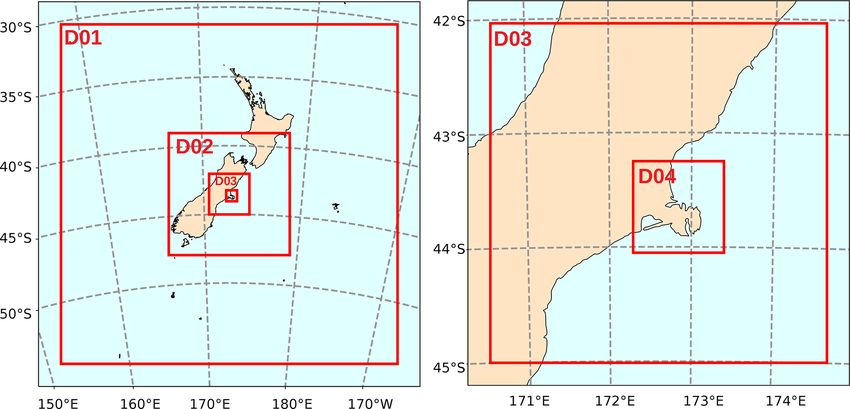
14092                                                                         B. Nathan et al.: Inferring PM2.5 emissions sources

Figure 1. Map of Christchurch with the locations of the PM instruments and AWSs as deployed during the MAPM field campaign in 2019.
The location of Christchurch within New Zealand is shown in the top right corner as indicated by the red box. © OpenStreetMap contributors
2020. Distributed under the Open Data Commons Open Database License (ODbL) v1.0.

ture were measured using several automatic weather sta-                subtracted from the concentrations measured within the do-
tions (AWSs). Three AWSs were installed specifically for the           main. The approach to define the background can become
MAPM campaign on the outskirts of Christchurch (Fig. 1).               complex. Additionally, to relate the measurements against
These measurements were complemented by data provided                  the emissions estimates, a transformation operator must be
from 13 AWSs that are permanently installed and operated               used to put them into the same unit space. In this context,
by the New Zealand MetService and the National Insti-                  the transformation operator is defined by the source–receptor
tute of Water and Atmospheric Research (NIWA). Because                 relationships at any measurement site, which in turn are es-
the AWSs were operated by several different institutions,              tablished through the use of an atmospheric transport model
the variables recorded and the rate at which the data were             to identify the potential source regions on the ground con-
recorded differ throughout the network. All AWSs measured              tributing to any particular concentration measurement. The
wind speed and direction, temperature, and relative humidity,          prior emissions map, the measured enhancements, and the
at a temporal sampling period ranging between 1 and 10 min             transformation operator are each integrated into the Bayesian
– for consistency, all meteorological measurements from all            inverse equation to calculate an updated posterior emissions
AWSs were averaged to a 10 min temporal resolution.                    estimate map. We expand upon the details of this procedure
                                                                       in the following sections.
                                                                          As described above, given the meteorological input re-
3   Inverse modelling framework                                        quired to establish the source–receptor relationships, to esti-
                                                                       mate the PM emissions map, the inverse model must achieve
As shown in Fig. 2, the inverse modelling framework derives            a balance between the emphasis given to the prior emissions
its solution by combining several components. In general,              map and the PM concentration measurements. This balance
the measured concentrations are being optimized against the            is achieved by prescribing adequate uncertainty to the prior
first-guess prior emissions map. However, the measured val-            and to the measurements. For a single inversion performed,
ues of interest need to be just the enhancements from the              i.e. a posterior emissions map derived for a single time step,
region of interest, so an appropriate background value rep-            where a prior emissions map and a series of measurements
resenting contributions from outside of the domain must be             are provided as input, the quality of the posterior emissions

Atmos. Chem. Phys., 21, 14089–14108, 2021                                                https://doi.org/10.5194/acp-21-14089-2021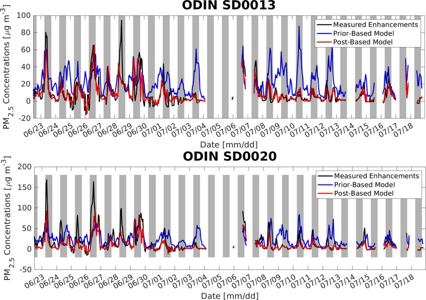
B. Nathan et al.: Inferring PM2.5 emissions sources                                                                               14093

Figure 2. Overview of the inverse model set-up, its inputs, and its outputs as used and described in this study.

map (driven by the derived uncertainties) is likely to depend             from 172.29 to 173.4◦ E, with a horizontal resolution of 1 km
heavily on the quality of the prior emissions map, as reported            (cf. 27, 9, and 3 km in Guo et al., 2018) and a temporal res-
by Guo et al. (2018), which is consistent with previous liter-            olution of 10 min, was used as input to FLEXPART-WRF
ature (e.g. Gurney et al., 2005; Lauvaux et al., 2016).                   (Sect. 3.1.2).
                                                                             Simulated temperatures and wind speed were compared
3.1     Transport modelling                                               to observations (Appendix A2), and it was found that while
                                                                          WRF has some difficulty in reproducing observed night-time
In this study, the coupled LPDM FLEXPART–WRF model                        temperatures during low-wind-speed conditions, WRF gen-
version 3.3.2 (Brioude et al., 2013) is used as the atmo-                 erally captures the meteorological conditions of the region
spheric transport model that relates changes in emissions                 within the typically expected uncertainties. For example, the
to changes in concentrations, i.e. the source–receptor rela-              overestimation of the wind speeds near the surface in the
tionships (SRRs). FLEXPART-WRF combines the Weather                       WRF model are a known feature of the model (e.g. Shimada
Forecast and Research Model (WRF) version 4.0 (Ska-                       et al., 2011), and uncertainties remain on whether this bias
marock et al., 2019) and the FLEXPART model (Stohl et al.,                is caused only under specific conditions. Overall, we have
2005; Pisso et al., 2019) version 9.                                      confidence in the WRF model to use it as the driver for the
                                                                          dispersion model in the inversion formulation, using an ap-
3.1.1    Weather Research and Forecasting Model – WRF                     propriate characterization of the relevant uncertainties.
A challenge for modelling PM dispersion in an urban envi-                 3.1.2   FLEXPART-WRF and footprint calculations
ronment is accurately representing the meteorological con-
ditions and capturing, with high fidelity, the influence of               Using the meteorological output at a horizontal resolution
terrain under complex topography on the meteorology (Fay                  of 1 km from WRF (Sect. 3.1.1 and Appendix A1) as input,
and Neunhäuserer, 2006). For the purposes of this study, we               FLEXPART-WRF was used to derive the source–receptor re-
use WRF (Skamarock et al., 2005), a widely used numerical                 lationships (SSRs) by running the LPDM backward in time;
weather prediction model designed for operational weather                 e.g. particles were released from a measurement location to
forecasting as well as atmospheric research.                              identify potential upwind sources. As the current version of
   WRF version 4.0 was employed to simulate the meteo-                    FLEXPART-WRF does not support the direct simulation of
rological fields with four nested domains over Christchurch               PM2.5 concentrations, the FLEXPART-WRF simulation was
(Fig. A1). The model simulation set-up is describe in Ap-                 set up to simulate the particles as passive tracer air parcels
pendix A1. Overall a total of 32 WRF simulations were per-                without considering chemical reactions and dry or wet de-
formed, covering the period from 21 June to 18 July 2019.                 position. To avoid the complications of wet deposition, we
Each simulation was initialized daily at 00:00 UTC and ran                exclude rainy periods from our study (see below). The loss
for a total of 72 h, with the first 48 h allocated for spin up,           processes via chemistry and dry deposition were not consid-
which was discarded from the final output files that were                 ered as explained in the following.
used as input to FLEXPART-WRF. Furthermore, only the
meteorological output from domain 4 (d04), spanning the                      – Air chemistry in Christchurch in winter is such that
latitude range from 44.05 to 43.25◦ S and longitude range                      there is little, if any, chemical transformation of PM be-

https://doi.org/10.5194/acp-21-14089-2021                                                 Atmos. Chem. Phys., 21, 14089–14108, 2021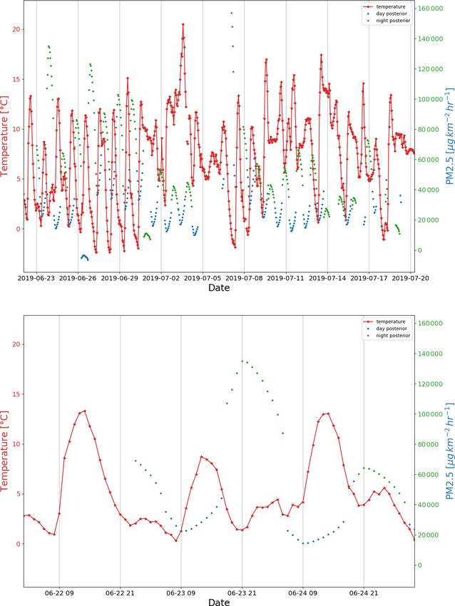
14094                                                                  B. Nathan et al.: Inferring PM2.5 emissions sources

      cause of the low background concentrations of sulfur       the time of this study, there was insufficient Christchurch-
      dioxide (Coulson et al., 2016).                            specific bottom-up data available to incorporate a temper-
                                                                 ature dependency into the prior; however we acknowledge
  – While loss through dry deposition is possible, it is un-     that a robust handling of this could lead to improved pos-
    likely to play a large role in Christchurch. There are no    terior emissions estimates and should thus be considered in
    studies in Christchurch to confirm this assumption, but      future investigations. Across the whole domain, home heat-
    a study performed in California (Herner et al., 2006)        ing contributes 72 % to the total PM2.5 emissions on a typ-
    under similar wintertime inversion conditions modelled       ical winter day, while traffic and industry emissions only
    deposition rates for particles of a size between 0.1 and     contribute 20 % and 8 % to the total emissions, respectively
    3 µm to be between 2.4 × 10⁻⁴ and 4.34 × 10⁻⁴ m s−1 .        (Tim Mallett, ECan, personal communication 2020). The rel-
    During the evening hours when mixing depths are on           atively high amount of emissions coming from home heating
    the order of 50 m, these velocities suggest deposition       was a primary driver for the measurement campaign being
    timescales of 58 and 32 h. A study by Jeanjean et al.        conducted during the winter.
    (2016) also found that deposition rates of PM2.5 are low,       For this study, ECan provided an estimate for the average
    especially in winter.                                        PM2.5 emission of a wood burner based on 2018 census data,
Although these loss processes were not included in this study,   issued permits for wood burners, and estimated emissions per
we acknowledge potential small uncertainties to be intro-        burner type. It should be noted that ECan formulates their
duced to the posterior emissions maps, which will also be        estimate with an eye towards the worst-case scenario, as this
acknowledged in Sect. 4. Future studies will need to con-        would be most relevant to negative human health impacts,
sider the inclusion of these loss processes depending on the     and thus the prior emissions maps used here essentially act
environment and PM2.5 sources in the city of interest.           as the upper limit of estimated PM2.5 emissions.
   To establish the SSR for each hourly mean PM measure-            The 2018 census data were compiled based on a set of
ment, FLEXPART-WRF simulations were initiated at the end         questions taken to the Christchurch community regarding
of the 1 h period (noting that FLEXPART-WRF is running           whether or not they used wood for home heating. The census
backward in time). Then, during the 1 min period, 10 000 par-    data were provided on statistical areas, which are irregularly
ticles were released continuously from 49 receptor locations     shaped polygons of various sizes covering the Christchurch
that correspond to the measurement sites described in Sect. 2    city domain. To estimate the PM emissions from households
and traced backwards in time over a 24 h period to establish     in Christchurch, the number of households using a wood
their potential sources. The release altitude was set to 2 m     burner was multiplied by the average PM2.5 emissions per
for all releases, and the FLEXPART-WRF output was saved          wood burner. Of these total household emissions, 73 % were
every 30 min on the same grid as the WRF output was pro-         then used as an estimate for PM2.5 emissions on a typical
vided, i.e. same domain with a 1 km horizontal resolution.       winter night. Here the assumption is that the type of wood
Overall, FLEXPART-WRF was run independently for each             burners and the percentage of active burners on a given night
hour of the 31 d spanning the period from 22 June to 18 July     remain consistent across the city. The industry emissions for
2019.                                                            the top 13 emitters were calculated based on discharge esti-
   FLEXPART-WRF output, provided in units of residence           mates from ECan, and together they represent around 77 %
time (seconds), can be used to identify the origin of emis-      of estimated industrial PM2.5 emissions for the Christchurch
sions sources that contribute to the concentrations “mea-        airshed. Vehicle emissions were also provided by ECan and
sured” at the receptor. We use the FLEXPART-WRF output           are based on 2014 data from the Christchurch Transport
to create “footprints” that describe the backwards-in-time lo-   Model, and emission factors were derived from the vehicle
cal contributions to any in situ measurement by integrating      emissions prediction model that was developed by the New
over 12 h of output and over a 60 m thick surface layer. A       Zealand Transport Agency.
time period of 12 h was chosen to be enough time for the            To derive hourly estimates of PM2.5 emissions, the total
particles to traverse the domain even under weak wind con-       24 h emissions were divided according to the estimated con-
ditions, and 60 m was chosen as the integration height to        tribution of that hour to the total daily emissions for each
be high enough to capture any elevated emissions sources.        of the three sources separately – these estimates were pro-
These footprints define the transport matrix (H), which is       vided by ECan for home heating and traffic. Due to a lack
used to relate the emissions in flux space to the measure-       of any detailed information about the timing of the emis-
ments in concentration space, as shown later in Eq. (1).         sions released by industries, it was assumed that the indus-
                                                                 try emissions were released evenly throughout the 24 h pe-
3.2   Prior PM2.5 emissions estimates                            riod. Overall the highest emissions occurred during nighttime
                                                                 when people were at home starting their fires.
Derived bottom-up emissions estimates used in this study            The household-based emissions per statistical area and the
include PM2.5 emissions sources from (i) traffic, (ii) indus-    traffic emissions were rasterized onto a 10 m by 10 m New
try (the top 13 industries only), and (iii) home heating. At     Zealand Transverse Mercator 2000 (NZTM2000) grid. In-

Atmos. Chem. Phys., 21, 14089–14108, 2021                                        https://doi.org/10.5194/acp-21-14089-2021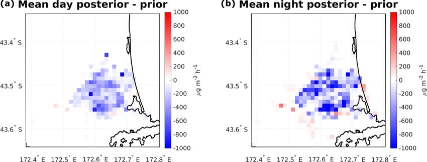
B. Nathan et al.: Inferring PM2.5 emissions sources 14095
dustry emissions were added as point sources on this grid. To estimate the background PM2.5 concentration at any
During the rasterization, the conversion from grams per given hour, 1 min resolution PM2.5 concentration measure-
meshblock (statistical area) to grams per square metre was ments from the ODIN and 5 min resolution of the wind data
calculated. The NZTM2000 grid was interpolated and pro- were used in the following procedure.
jected onto the fourth WRF domain (Fig. A1), using conser-
vative interpolation which preserves the total emissions. The 1. For each AWS site, a range of wind direction angles
bottom-up estimate for PM2.5 emissions in Christchurch over were determined that correspond to the wind flowing
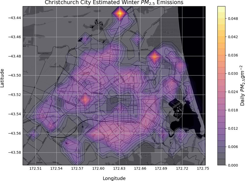
a 24 h period is shown in Fig. 3, representing emissions on a into the domain (Table 1).
typical winter day. 2. Using PM2.5 data from the ODIN corresponding to each
The hourly resolution maps are used to construct the final AWS site, and the respective 5 min resolution wind data,
prior emissions map that is used in the Bayesian inversion we select all PM2.5 measurements that correspond to the
equation. First, for any given hour with a given set of hourly range of wind directions that define air flowing into the
measurements, the corresponding emissions map is a mean domain.
emissions map across the preceding 12 h of emissions. This
averaging is done to match the 12 h length of the footprints, 3. For each site, the PM2.5 measurements that had been
so that it is appropriately representative. Then, the definitive selected in the previous step were then screened for
prior emissions map is a mean of each of these hourly emis- episodic short-term local emissions of PM based on
sions maps across every hour in the inversion period. (i) whether the change in PM2.5 from one minute to
the next is greater than 50 µg m−3 and (ii) whether the
3.3 Determination of the background concentrations PM2.5 measurement at time t exceeds 2σ , where σ is
the standard deviation calculated from the 1 min data,
Since this study focuses on constraining the emissions within for each hour of available measurements.
the boundary of the city of Christchurch, the concentra-
tion measurements being provided as input to the inverse 4. All remaining PM2.5 concentration measurements from
model should similarly only reflect the emissions coming all sites are combined into one time series and, because
from within the boundary of the city; i.e. they should exclude the temporal resolution of the concentration measure-
any contribution from emissions sources located outside the ments used by the inverse model is hourly, hourly av-
city. As a result, any potential influx of PM into the domain erages are calculated from these remaining measure-
(here referred to as the background) needs to be subtracted ments.
off each concentration measurement taken within the city
5. As a final step, and to remove any remaining local influ-
domain, leaving only concentrations that are a function of
ences, a 10 d running median of the hourly time series
in-domain emissions, hereafter referred to as enhancements.
is computed. This running median value is then used as
Defining the background air mass is often one of the most
the background PM2.5 concentration across the whole
difficult yet important challenges during the inversion for-
domain for a given hour of the day.
mulation (e.g. Göckede et al., 2010; Lauvaux et al., 2016). In
the CO2 community, for example, this is often achieved by Figure 4 shows a time series comparison of the adjusted
selecting a measurement site to act as a background based on background value against two of the measurement sites lo-
wind direction (e.g. Kort et al., 2012; McKain et al., 2012; cated near the centre of the city. These have been chosen
Lauvaux et al., 2016). Here, we adapted the approach to be to be ODIN sites SD0013 and SD0020. The new presented
applied to determine the background PM2.5 concentrations. methodology has created a background time series that does
During the MAPM measurement campaign and to esti- not appear to contain any of the large spikes from stochastic
mate the inflow of PM into the domain, several sensors were local events, while still containing real, apparently reason-
deployed on the perimeter of the city. Measurements from able background variations.
five of these “background” sites were used, together with
wind direction measurements, to estimate the background 3.4 Bayesian inversion calculation
PM concentrations flowing into the city. Specifically, the city
of Christchurch was divided into four quadrants with Hagley Given the prior flux estimates of the emissions and the mea-
Park at the centre. A total of five AWS–ODIN pairs were se- sured enhancements, the optimal emissions flux map is com-
lected along the perimeter to determine the background PM puted using the Bayesian inversion calculation, following the
concentrations. The five sites are marked in Fig. 1, as named formula in Tarantola (2005):
sites. To determine whether or not the wind was blowing into
x = x0 + BHT (HBHT + R)−1 (y − Hx0 ). (1)
the domain, the angle between the location of the AWS and
Hagley Park was estimated. This angle corresponds to a wind Here, x is the posterior flux map, x0 is the prior flux map, B
direction under which air is being advected into the domain. is the prior error covariance matrix, H is the influence func-
tion (more specifically the transport matrix, containing the
https://doi.org/10.5194/acp-21-14089-2021 Atmos. Chem. Phys., 21, 14089–14108, 2021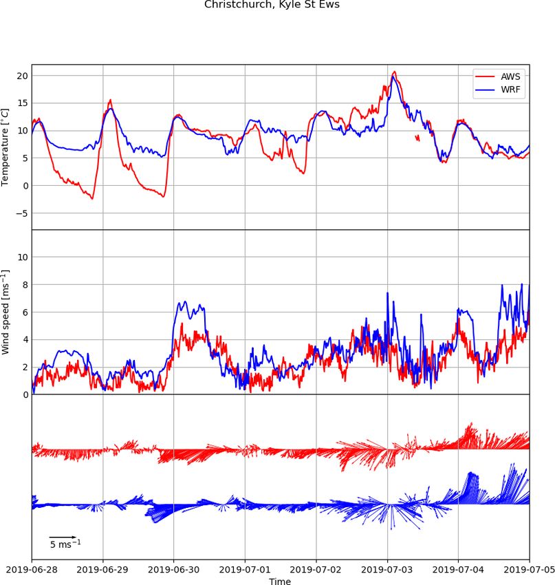
14096                                                                            B. Nathan et al.: Inferring PM2.5 emissions sources

                                                                                                                        .

Figure 3. Bottom-up emissions map over Christchurch, interpolated onto the 1 km WRF grid and used as the prior for the inversion calcula-
tion. PM2.5 emissions sources include (i) household heating, (ii) traffic, and (iii) industry. Contour lines are shown for every 0.002 g m−2 of
PM2.5 .

Table 1. Wind direction angles that define air blowing into the city for each measurement site at the perimeter of the city.

                             Halswell     New Brighton             Sugarloaf          Belfast    Christchurch Airport
                        22.5◦ ± 22.5◦     67.5◦ ± 22.5◦     168.75◦ ± 22.5◦     225◦ ± 22.5◦          303.75◦ ± 22.5◦

12 h footprints for each hourly measurement), R is the er-                still maintain some spatial error correlations with the under-
ror covariance matrix for the observations, and y is the one-             standing that they are necessary to keep the inverse problem
dimensional matrix of hourly averaged measured enhance-                   regularized and thus to prevent a divergence of the solution at
ments.                                                                    points where the inverse model grid overlaps with the recep-
   The posterior error matrix is defined as                               tor sites, called the “colocalization problem” (Bocquet, 2005;
                                                                          Saide et al., 2011). To account for the possibility that the real
A−1 = B−1 + HT R−1 H.                                            (2)      structure of the error correlations is not properly captured by
   The errors on the prior flux estimates are assigned in a               these additional spatial correlations, and that in fact we may
manner similar to what has been described in Nathan et al.                be overestimating the correction, we do include some results
(2018) and Lauvaux et al. (2016). The error covariance ma-                without these spatial correlations later in Fig. 5. For the er-
trix for the prior fluxes, B, contains the variances for every            ror covariance matrix for the observations, the variances are
grid point in the domain along the diagonal and the cross-                defined as the square of the measurement uncertainties that
correlation terms in the off diagonals. The variances are de-             are provided with the data sets (Dale et al., 2021). The off-
fined as the square of the root mean square (rms) values at               diagonal elements of the covariance matrix are all set to zero;
each grid point of the flux map, and the rms values are set               i.e. all measurements at different locations and times are con-
to be 50 % of the corresponding flux value. The covariances,              sidered to be independent from one another.
representing the spatial error correlations, are then defined
using an exponential decay function with a 1 km correlation
length. Here, we have set the correlation length to match the
grid-cell size in the domain, to allow for more independence
in the allocation of emissions adjustments during the inver-
sion process. However, even with this near independence, we

Atmos. Chem. Phys., 21, 14089–14108, 2021                                                   https://doi.org/10.5194/acp-21-14089-2021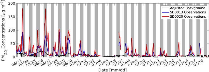
B. Nathan et al.: Inferring PM2.5 emissions sources                                                                             14097

Figure 4. A time series comparing the adjusted background value against two measurement sites located near the city centre.

4   Inversion calculation using measurements obtained                  preceding 12-hourly estimated emissions maps, a length that
    during the MAPM field campaign                                     was chosen to correspond to the 12 h footprints for the mea-
                                                                       surements at that hour. A scale factor is derived for the cre-
                                                                       ation of the corresponding “hourly” time series of posterior
An inversion calculation was performed using the measure-              values, since only one posterior map is computed per day-
ments obtained during the MAPM field campaign (Sect. 2).               time or nighttime period. This scale factor is defined as the
The period for the inversion was chosen to be from 22 June             proportion of the domain sum of the posterior emissions map
2019, 12:00 UTC to 18 July 2019, 24:00 UTC. The inversion              divided by the domain sum of the mean prior emissions map
was then run for the “daytime” and “nighttime” separately,             (across all included hours) used in the inversion for the given
where daytime was defined from 06:00 to 18:00 LT (18:00–               daytime or nighttime period.
06:00 UTC, excluding 06:00 UTC) and nighttime from 18:00                  In addition, posterior emissions time series where (i) 1 km
to 06:00 LT (06:00–18:00 UTC, excluding 18:00 UTC). One                spatial correlation was included and (ii) no spatial correlation
posterior map per day was computed for each daytime or                 was considered in the construction of the prior uncertainty
nighttime period. The overall structure and components of              matrix are also shown in Fig. 5. As explained in Sect. 3.4, the
the MAPM tool, including the inverse model system, are                 inclusion of some non-zero spatial correlation value was im-
shown schematically in Fig. 2.                                         plemented to address the “colocalization problem” that can
    Because rain is known to wash out PM from the atmo-                lead to spurious corrections of the prior at grid cells where
sphere (e.g. Atlas and Giam, 1988), which would lead to ar-            measurement sites are located (Bocquet, 2005). Furthermore,
tificially low measurements and therefore would bias the in-           the tendency for residential areas to be in spatial proximity
version results, all hours during which rain occurred were             to each other gives some physical justification for the inclu-
removed from the data set. The 12 h following any rain                 sion, in our problem, of a non-zero spatial correlation in the
event were also removed from the data set, to prevent over-            prior uncertainty matrix, as well. That said, we acknowledge
counting in our inversion set-up which uses 12 h footprints;           that this is an imperfect metric to describe the system and
i.e. this allows the emissions to “build back up” enough in the        that our description of the correlations may not adequately
atmosphere to match the 12 h integrated footprints that are            capture the complexity of the real situation. As a result, we
used in this study. The “rainy hours” were identified by using         include the dashed magenta line in Fig. 5 to show what the
data from the AWS that is installed close to the city centre,          posterior results would be without the addition of this spa-
at Kyle Street (purple cross in Fig. 1), wherein any hour that         tial correlation on the uncertainty. It shows that our system
recorded any nonzero precipitation value was deemed to in-             may be slightly overestimating the downward adjustment in
dicate a potential rainfall event in the area during that hour.        the posterior emissions compared to the prior. However, this
The PM2.5 measurements at that hour and the following 12 h             difference in the adjustment is small enough such as not to
for all PM measurements at all sites were thus excluded from           dramatically change the conclusions we draw from this anal-
the analysis.                                                          ysis. For the remainder of the results section, we will thus
    The results of the inversion indicate a significant overes-        present the results that are based on including a prior uncer-
timation of the inventory estimates for PM2.5 emissions in             tainty matrix with a 1 km correlation length.
Christchurch. Figure 5 shows the time series comparison for               For both daytime and nighttime, the results indicate a 40 %
prior-based flux estimates compared with the posterior flux            to 60 % overestimation of the prior emissions compared to
estimates for the daytime and nighttime. The values shown              the posterior emissions. The impact of not including loss of
are sums across the entire domain, for either the prior or             PM due to chemistry and dry deposition may account for a
posterior maps. The prior map at any hour is a mean of the

https://doi.org/10.5194/acp-21-14089-2021                                             Atmos. Chem. Phys., 21, 14089–14108, 2021
14098 B. Nathan et al.: Inferring PM2.5 emissions sources
Figure 5. Time series of sum of the fluxes across the domain in the prior, posterior using a spatial correlation of 1 km, and posterior using no
spatial correlation, for the daytime and nighttime inversions.
small amount of this downward adjustment, as explained in As a result, the inventory comes with a large uncertainty that
Sect. 3.1.2. Rather, most of the observed posterior adjust- favours the possibility of an overestimation. Thus, the results
ment is believed to be an expected result following several of the inverse model adjusting to lower emissions in the pos-
assumptions that had been made when calculating the PM2.5 terior, as in Fig. 5, is viewed as sensible. Recent observing
inventory (Tim Mallett from ECan, personal communication, system simulation experiments (OSSEs) presented by Lau-
October 2020) as follows. vaux et al. (2020) indicate that an inversion set-up like the
one used here should be able to recover values close to the
– A total of 73 % of wood burners are active on a typi- true emissions if the prior fluxes are offset by as much as
cal night. The percentage was calculated from field sur- 20 %. However, large offsets above 40 % may not be able to
veys, where the “number of chimneys seen hot on a be fully recovered and may still require an extra correction.
given night” was recorded, which was then divided by In their study, a 40 % offset in the prior from the truth was
the respective number of households who reported us- still 18 % away from the truth after inversion. This may im-
ing a wood burner to heat their home (obtained from ply that the apparent overestimation in Christchurch’s prior
census data). This results in the ratio of the number of emissions is still larger than our posterior results indicate.
wood burners active on a typical winter day. The nighttime period is traditionally left out of inversion
analyses because of difficulties in the model to accurately
– The fuel use estimates assume around 10 h of use per capture the nocturnal boundary layer (Geels et al., 2007;
day for wood burners. This can be an overestimation Steeneveld et al., 2008). For example, Lac et al. (2013) found
as (i) new homes have more insulation than previous a positive bias of 5 ppm of CO2 in urban and suburban re-
houses; (ii) heat pumps are installed in new homes gions of Paris, which was attributed to a boundary layer
rather than wood burners, which lead to no PM emis- height error in the transport model. Despite that, we are in-
sions; and (iii) a smaller floor area or fewer occupants cluding the results from the nighttime inversion because the
would reduce the burning time. residuals for the nighttime analysis compared to the daytime
analysis show overall good agreement, as seen in Fig. 5.
– All wood burners over 1.0 g kg−1 are combined into one Additionally, the nighttime is of particular interest to this
emission factor category, though a future version of the investigation, as the primary source of PM2.5 emissions in
inventory separates out 1.0–1.5 g kg−1 from those over Christchurch is home heating (Sect. 3.2), which is typically
1.5 g kg−1 , which could further lower emissions esti- used in the evening when the ambient temperature is at its
mates. lowest. Thus, the results from the nighttime inversion are
presented here as well, with the note that they should be ac-
– There is ambiguity in the underlying census data used cepted with caution.
to tally the number of active burners or the time they The nighttime posterior values inferred by the inversion
are used for, which only asks a homeowner whether and shown in Fig. 5 indicate generally more variable emis-
they use a wood burner but does not include a question sions from night to night compared to the results from the
around whether or not they have an alternative heating daytime inversions. Some of this variability can be explained
method or an estimate of the average amount of time in part to originate from the transport model uncertainty re-
that they use the heating.
Atmos. Chem. Phys., 21, 14089–14108, 2021 https://doi.org/10.5194/acp-21-14089-2021B. Nathan et al.: Inferring PM2.5 emissions sources 14099
Figure 6. Example time series for in-city measurement sites showing the prior-based concentrations, the measured enhancements (i.e. PM2.5
concentration measurements where the background has been removed), and the posterior-based concentrations, showcasing the improvement
provided by the inversion. Grey shaded areas indicate nighttime hours.
lated to the nocturnal boundary layer height, as explained space. Then, for any given measurement site, these time se-
above. In general, however, the result present in the daytime ries can be plotted. By noting where the red line (posterior
inversions, i.e. that the posterior estimates are significantly estimates) matches the measurements (black line) better than
lower than the corresponding priors, is upheld. the blue line (prior estimates), we see the adjustments by the
We also acknowledge the presence of some negative emis- inversion at this measurement site.
sions values in some grid cells of the posterior. This may oc- In general, the concentrations derived from the posterior
cur in situations where the observed enhancement values for converge from the prior concentrations towards the measured
the city are made negative due to the uncertainties inherent enhancements, which indicates that the inversion is work-
in an imperfect background characterization, as is the case ing insofar as the uncertainty on the measurements is much
during the daytime inversion for 26 June. However, negative smaller than that on the prior fluxes, and therefore the mea-
pixels may also naturally result simply from the analytical surements have a strong influence on the posterior result. The
solution to the Bayesian inversion equation we implement. model has difficulty with capturing some of the strong spike
This is also the case in our situation, yet we would consider events seen in the measurements, especially during night-
the implementation of a positivity constraint to be an unjus- time, but overall it is able to follow the general variability
tifiable manipulation to the mathematical system. As a re- seen in the enhancement time series, across all instruments
sult, the mean posterior grid for the daytime inversions con- (Fig. 6). The events of high PM2.5 concentrations correspond
tains 28 negative pixels out of the 9100 total, and the mean to periods of low wind speeds and low temperatures. How-
nighttime posterior grid contains 29 negative pixels out of the ever, these enhancements could also be the result of a lo-
9100 total. These negative pixels comprise such a small pro- cal source, which either is not well-resolved by the inverse
portion of the domain that they are not considered to materi- model due to the comparatively coarse 1 km resolution or is
ally change our conclusions. Rather, we make note of them a consequence of having instruments positioned too close to
here in the interest of transparency. the surface.
Figure 6 shows two time series plots from measurement Figure 7 takes a broader look at the temperature relation-
sites towards the centre of the domain (near the city cen- ship of the system, showing the temperature time series ob-
tre). By multiplying the prior or posterior flux maps by the tained from an AWS located near the city centre (Kyle Street)
transport operator H, we can compare the prior and posterior plotted together with the sum of the daytime and nighttime
estimates against the measurements directly in concentration posterior emissions. The top panel shows this comparison
https://doi.org/10.5194/acp-21-14089-2021 Atmos. Chem. Phys., 21, 14089–14108, 202114100 B. Nathan et al.: Inferring PM2.5 emissions sources
Figure 7. Hourly mean temperature as obtained from the AWS located at Kyle Street, together with the sum of the inferred PM2.5 emissions
for daytime (blue) and nighttime (green).
across the entire analysis period, while the bottom panel To understand where the adjustments are being made spa-
shows a zoom-in of a particular period. The posterior emis- tially, we include maps of the mean difference between the
sions are, as expected, anti-correlated with temperature; i.e. posterior and the prior over the course of the analysis period,
during nighttime when the temperature is low, the emissions for both daytime and nighttime, as shown in Fig. 8. The cor-
increase and vice versa. This is consistent with the primary rection for apparent overestimates in the prior is distributed
driver of emissions in Christchurch being the use of wood throughout the city during both day and night. Also, several
burners. Also, during warm periods, e.g. between 2 and 5 of the large point sources present in the prior (see the Fig. 3),
July, while following a diurnal cycle, the emissions are rather have had many of the corrections attributed to them. This is a
low, reflecting that the use of wood burners was reduced dur- consequence, in part, of the flux uncertainty scaling with the
ing that period. These results give us confidence that the in- prior emissions, as the inversion will preferentially attribute
verse model is producing reasonable results. corrections to grid points with large uncertainties. Since the
overwhelming majority of emissions are expected to come
Atmos. Chem. Phys., 21, 14089–14108, 2021 https://doi.org/10.5194/acp-21-14089-2021B. Nathan et al.: Inferring PM2.5 emissions sources 14101
Figure 8. The mean difference between the posterior and prior maps in the daytime (a) and nighttime (b) across the full inversion period.
The mean prior and posterior were calculated from the 10 daytime and nighttime maps, respectively.
from home heating, it can be assumed that a large majority measurement stations at any particular hour, can be a signifi-
of the corrections may apply to that sector. However that does cant source of uncertainty, as well. Further, it is expected that
not rule out the possibility of misattributions in other factors the loss processes are only contributing a small uncertainty to
of the prior, as well (e.g. traffic and industry). the inferred emissions maps for Christchurch during winter;
Furthermore, the results reveal an apparent increase in however, the decision to not explicitly account for loss pro-
emissions in a ring just outside of the city, especially during cesses (specifically chemical or dry deposition, as discussed
nighttime. Given that these areas outside of the city had fewer in Sect. 3.1.2) will need to be given thorough reconsideration
measurement sites nearby, and thus fewer footprints overlap- in any future applications of the methodology described here
ping the regions with which to issue corrections, it is possible for cities other than Christchurch.
that these sites are simply reflecting under-representation in
the model. This may be evidenced by the fact that these ef-
fects are amplified at night, where the transport error is at its 5 Conclusions
highest due to the difficulties with accurately simulating the
nocturnal boundary layer. However, it is also possible that The PM2.5 inversion system established through the MAPM
these are real sources of emissions that are not well-captured project using Christchurch, New Zealand, as its test bed has
and identified by the inventory because of, for example, new been shown to be an effective system for assessing aerosol
developments that may have been built after the information emissions in the urban environment using a large number of
for the construction of the prior was gathered in 2018. measurement sites. The system was applied to measurements
The results of the presented study are considered to pro- obtained during the MAPM field campaign during the winter
vide an improved estimation of the quantity and distribution of 2019.
of PM2.5 emissions from the region during the wintertime The inversion results suggest what appears to be a system-
2019 measurement campaign. However, the study still con- atic overestimation in the prior emissions estimates of PM2.5
tains several substantial sources of uncertainty that may have for Christchurch, which is in the range of 40 %–60 %, but
affected the results and should therefore be acknowledged. which may be higher due to limitations of the inverse cal-
Although they have been identified throughout this paper, we culation in situations with such a large mismatch. This con-
restate them here for clarity and transparency. First, the low clusion is in line with what would be expected, considering
sampling heights for the majority of the instruments (46 % several of the assumptions that had been used in the calcula-
of instruments at or below 3 m above the ground) open the tion of the inventory on which the prior emissions estimate is
door for local turbulence to have impacted the measurements; based. The fact that the prior emissions estimate was created
future studies should make every effort to record measure- with an eye towards a worst-case scenario, to err on the side
ments at higher altitudes. Furthermore, the modelled atmo- of caution for human health, means that an overestimation of
spheric transport always involves some potentially impact- some significance would have been expected. Site compar-
ful amount of uncertainty. Beyond the characterized mis- isons against the measurements in concentration space ap-
matches with the winds, a future study could become more pear to give further support to the idea that the inversion is
robust by including in situ measurements of the boundary capturing the real trends seen in the measured enhancement
layer, as well. Additionally, the characterization of the in- data.
flow, used to define the background PM2.5 values across the The presented results constitute a proof-of-concept study
for inferring PM emissions sources on a city scale, using
https://doi.org/10.5194/acp-21-14089-2021 Atmos. Chem. Phys., 21, 14089–14108, 202114102 B. Nathan et al.: Inferring PM2.5 emissions sources Christchurch as a test bed for high-measurement-density We have additional ideas that could improve future efforts aerosol urban inversions, to provide city officials with near- to implement MAPM more robustly, as well. First, such in- real-time assessments of surface emissions. We successfully vestigations may benefit from developing a more robust prior demonstrate the feasibility of the system, and our investiga- that incorporates some temperature dependency, especially if tion has itself identified potential areas of improvement in the again being implemented in an area where wood burners are current emissions estimates for Christchurch. This study lays the primary source of wintertime PM2.5 emissions. Addition- the groundwork for future investigations that may seek the ally, future efforts focused outside of Christchurch may need same goal in disparate urban environments around the globe. to more explicitly handle secondary organic aerosols in the We assessed the different sources of uncertainty inherent transport model. in our approach. One of the largest areas is the transport model. Thus, the logical next step is going to be to implement a higher-resolution model that can better characterize wind flows and turbulence at urban scales: the PArallelized Large- eddy simulation Model (PALM; Maronga et al., 2015). This will be coupled to WRF and, eventually, will include chem- istry in the model to capture the effects of aerosol chemistry and deposition. The coupled WRF–PALM system, which has been developed by Lin et al. (2020), will be better able to simulate air flow (including, for example, effects of turbu- lence and diffusivity) in complex urban terrains and would provide higher-resolution output (10 m or finer, compared to the current 1 km resolution). Atmos. Chem. Phys., 21, 14089–14108, 2021 https://doi.org/10.5194/acp-21-14089-2021
You can also read