The neural basis of the blood-oxygen-level-dependent functional magnetic resonance imaging signal
←
→
Page content transcription
If your browser does not render page correctly, please read the page content below
Published online 2 August 2002
The neural basis of the blood-oxygen-level-dependent
functional magnetic resonance imaging signal
Nikos K. Logothetis
Max Planck Institute for Biological Cybernetics, Spemannstrasse 38, 72076 Tübingen, Germany
(nikos.logothetis@tuebingen.mpg.de)
Magnetic resonance imaging (MRI) has rapidly become an important tool in clinical medicine and biologi-
cal research. Its functional variant (functional magnetic resonance imaging; fMRI) is currently the most
widely used method for brain mapping and studying the neural basis of human cognition. While the
method is widespread, there is insufficient knowledge of the physiological basis of the fMRI signal to
interpret the data confidently with respect to neural activity. This paper reviews the basic principles of
MRI and fMRI, and subsequently discusses in some detail the relationship between the blood-oxygen-
level-dependent (BOLD) fMRI signal and the neural activity elicited during sensory stimulation. To exam-
ine this relationship, we conducted the first simultaneous intracortical recordings of neural signals and
BOLD responses. Depending on the temporal characteristics of the stimulus, a moderate to strong corre-
lation was found between the neural activity measured with microelectrodes and the BOLD signal aver-
aged over a small area around the microelectrode tips. However, the BOLD signal had significantly higher
variability than the neural activity, indicating that human fMRI combined with traditional statistical
methods underestimates the reliability of the neuronal activity. To understand the relative contribution
of several types of neuronal signals to the haemodynamic response, we compared local field potentials
(LFPs), single- and multi-unit activity (MUA) with high spatio-temporal fMRI responses recorded simul-
taneously in monkey visual cortex. At recording sites characterized by transient responses, only the LFP
signal was significantly correlated with the haemodynamic response. Furthermore, the LFPs had the larg-
est magnitude signal and linear systems analysis showed that the LFPs were better than the MUAs at
predicting the fMRI responses. These findings, together with an analysis of the neural signals, indicate
that the BOLD signal primarily measures the input and processing of neuronal information within a region
and not the output signal transmitted to other brain regions.
Keywords: functional magnetic resonance imaging; monkey; local field potentials; multi-unit activity;
action potentials; synaptic activity
1. INTRODUCTION we need repeated, conjoined anatomical and physiological
observations of the connectivity patterns at different
Modern in vivo imaging is one of medicine’s most exciting
organizational levels. In vivo imaging is an ideal tool for
success stories. It has optimized diagnostics and enabled
such observations, and is currently the only tool that can
us to monitor therapeutics, providing not only clinically
link perception, cognition and action with their neural
essential information but also insight into the basic mech-
substrates in humans.
anisms of brain function and malfunction. Its recently
In this review, I will first very briefly describe the history
developed functional variant has had an analogous impact
and basic principles of modern imaging techniques, and
in a number of different research disciplines ranging from
then concentrate on the application of MRI to the study
developmental biology to cognitive psychology.
of the monkey brain. Emphasis will be placed on fMRI at
In the neurosciences, imaging techniques are indispens-
high spatio-temporal resolution and its combination with
able. Understanding how the brain functions requires not
electrophysiological measurements. Finally, the neural ori-
only a comprehension of the physiological workings of its
gin of the BOLD contrast mechanism of fMRI will be
individual elements, that is its neurons and glia cells, but
discussed.
also demands a detailed map of its functional architecture
and a description of the connections between populations
of neurons, the networks that underlie behaviour. Further- 2. BASIC PRINCIPLES AND HISTORY
more, the functional plasticity of the brain, that is reflected
(a) Neuronal activity, energy metabolism and
in its capacity for anatomical reorganization, means that
brain imaging
a mere snapshot of its architecture is not enough. Instead,
Most current imaging techniques, in particular those
used to assess brain function, capitalize on the intercon-
nections among CBF, energy demand and neural activity.
One contribution of 14 to a Discussion Meeting Issue ‘The physiology It is therefore worth devoting a few paragraphs to an intro-
of cognitive processes’. duction of some basic concepts. Although comprising only
Phil. Trans. R. Soc. Lond. B (2002) 357, 1003–1037 1003 2002 The Royal Society
DOI 10.1098/rstb.2002.1114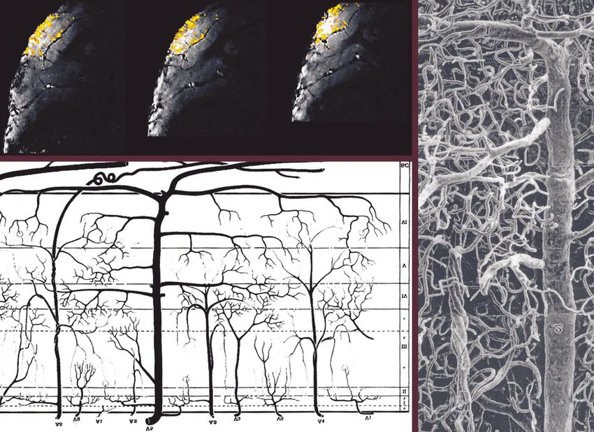
1004 N. K. Logothetis Neural basis of the BOLD fMRI signal

2% of the total body mass, the brain receives 12–15% of           regional coupling of the metabolic rate and neural activity
the cardiac output and consumes ca. 20% of the oxygen             came only from methods allowing local cerebral flow
entering the body (Siesjo 1978). The energy requirement           measurements. Although such methods had been used in
of the brain, or the CMR, is usually expressed simply in          conscious laboratory animals since the early 1960s
terms of oxygen consumption (CMRO2). This simplifi-               (Sokoloff 1981), a precise quantitative assessment of the
cation is possible because ca. 90% of the glucose                 relationship between neural activity and regional blood
(5 mg kg⫺1 min⫺1) is aerobically metabolized, and there-          flow was only possible after the introduction of the deoxy-
fore parallels oxygen consumption. CMRO2 is pro-                  glucose autoradiographic technique that enabled spatially
portional to neural activity and is four times greater in grey    resolved measurements of glucose metabolism in labora-
than in WM. At rest, the brain consumes oxygen at an              tory animals (Sokoloff et al. 1977). The results of a large
average rate of ca. 3.5 ml of oxygen per 100 g of brain           number of experiments with the 2DG method have indeed
tissue per minute (Siesjo 1978; Ames 2000). Approxi-              revealed a clear relationship between local cerebral acti-
mately 50–60% of the energy produced by this consump-             vation and glucose consumption (Sokoloff 1977).
tion supports electrophysiological function, as large                The first quantitative measurements of regional brain
amounts of energy are required for the maintenance and            blood flow and oxygen consumption in humans were per-
restoration of ionic gradients and for the synthesis, trans-      formed using the radiotracer techniques developed by Ter
port and reuptake of neurotransmitters (Siesjo 1978;              Pogossian et al. (1969, 1970) and Raichle et al. (1976).
Ames 2000). The remainder of the energy is used for               PET, the technology widely used today for clinical appli-
cellular homeostatic activities, including the maintenance        cations and research, followed (Ter Pogossian et al. 1975;
of the neuron’s relatively large membrane mass.                   Hoffmann et al. 1976) when Phelps et al. (1975) applied
   The brain’s substantial demand for substrates requires         the mathematical algorithms developed by Cormack
the adequate delivery of oxygen and glucose via the CBF.          (1973) for X-ray computed tomography; for a historical
The space constraints imposed by the non-compliant                review see Raichle (2000).
cranium and meninges require that the blood flow be suf-             PET images are spatial maps of the radioactivity distri-
ficient without ever being excessive. It is hardly surprising,    bution within tissues, and are thus analogous to the auto-
then, that there are very elaborate mechanisms regulating         radiograms obtained from 2DG experiments. With these
the CBF and that these mechanisms are closely coupled             PET images, it could be shown that maps of activated
with regional neural activity.                                    brain regions could be produced by detecting the indirect
   Angelo Mosso (1881) first demonstrated the correlation         effects of neural activity on variables such as CBF (Fox et
between energy demand and the CBF. He measured brain              al. 1986), CBV (Fox & Raichle 1986) and blood oxygen-
pulsations in a patient who had a permanent defect in the         ation (Fox & Raichle 1986; Fox et al. 1988; Frostig et
skull over the frontal lobes. Mosso (1881) observed a sud-        al. 1990).
den increase in pulsation, presumably due to an increase             At the same time, optical imaging using either voltage-
in the flow, immediately after the patient was asked to           sensitive dyes or intrinsic signals, that also relies on
perform simple arithmetic calculations. Interestingly,            microvascular changes, was being developed for animal
there was no concomitant increase in the patient’s heart          experiments and was used with great success to construct
rate or blood pressure as commonly measured at the fore-          detailed maps of cortical microarchitecture in both the
arm. Some years later, the neurosurgeon John Fulton               anaesthetized and the alert animal (Bonhoeffer & Grinvald
(1928) reported an increase in blood flow with increased          1996). Compared with PET, optical imaging has more
regional neural activation in the occipital lobe of another       limited coverage, but substantially better spatial reso-
patient with a bony defect that permitted the acoustical          lution, and it can be combined easily with other physio-
recording of the bruit from a vascular malformation.              logical measurements including single-unit recordings.
   Experimental evidence of the activity–flow coupling was        Finally, in recent decades another technology has emerged
provided by Roy & Sherrington (1890) after conducting             that could be used for conjoined anatomical and func-
experiments on laboratory animals. Roy & Sherrington              tional investigations. This new method was MRI, the tech-
indicated that some products of the brain’s metabolism            nology that offers a substantially better spatio-temporal
stimulated vasomotor activity that probably alters the            resolution than any other non-invasive method and which
regional vascular supply in response to local variations in       will be dealt with in the rest of this review.
the functional activity. In their seminal and remarkably
insightful study, they conclude that ‘…the chemical pro-                                    (b) MRI
ducts of cerebral metabolism contained in the lymph that          (i) Nuclear magnetism
bathes the walls of the arterioles of the brain can cause            The physical principles on which MRI is based are com-
variations of the calibre of the cerebral vessels: that in this   plex, and a thorough discussion of them is obviously
re-action the brain possesses an intrinsic mechanism by           beyond the scope of this article. For details, the interested
which its vascular supply can be varied locally in corre-         reader is referred to several excellent works on this topic
spondence with local variations of functional activity’           (Abragam 1961; Callaghan 1991; de Graaf 1998; Haacke
(Roy & Sherrington 1890, p. 105).                                 et al. 1999; Stark & Bradley 1999). Here, I provide a brief
   The study of Roy & Sherrington was later followed by           description of the basic concepts to make it easier to follow
the systematic investigations of Kety & Schmidt (1948),           the discussion of our own methodology that concludes
who introduced the nitrous oxide technique, a global flow         this review.
measurement method that initially seemed to disprove the             Imaging with NMR exploits the magnetization differ-
notion of a local coupling of cerebral flow and neural            ences that are created in a strong magnetic field. A rough
activity (Sokoloff 1960). Experimental verification of the        description of the phenomenon can be made with a classi-

Phil. Trans. R. Soc. Lond. B (2002)
Neural basis of the BOLD fMRI signal N. K. Logothetis 1005
(a) (b) (c)
phase-encoding direction
phase-encoding direction
1
normalized intensity
0.8
0.6
0.4
0.2
readout direction 0 2000 6000
4000 8000 readout direction
TR (ms)
(d) (e) (f)
phase-encoding direction
phase-encoding direction
1
normalized intensity
0.8
0.6
0.4
0.2
readout direction 0 50 100 150 200 250
TE (ms) readout direction
Figure 1. Relaxation curves for the GM and WM of the monkey brain. (a) Example of a proton-density image. The image
was collected with a multi-slice, multi-echo sequence using a FOV of 128 mm × 128 mm over a matrix of 256 × 256 voxels.
Sixteen such images are acquired using TR-values ranging from 50 to 8000 ms. (b) Average intensity change of voxels in
cortical (blue) and WM (red) regions as a function of repetition time, TR. T1 is defined as the time required for ca. 63% of
the remaining longitudinal magnetization to appear. The more ‘watery’ the tissue the longer its T1 relaxation time. The WM
(red curve, T1 = 1097 ms) relaxes faster than the GM (blue curve, T1 = 1499), so the former appears brighter in a typical T1-
weighted image than the latter (see figure 1c). The black trace shows the differences between the two curves. The maximum
contrast is obtained with a TR-value close to the T1-value of the tissue having the faster relaxation. (c) An example of aT1-
weighted image. (d ) An example of a spin-echo T2-weighted image. The relaxation times for different tissues were calculated
by collecting 16 such images differing in their TE-values. (e) The T2-relaxation curves for the cortex and WM, with the black
trace denoting the difference between the two. The T2-values are longer for small and shorter for large molecules, and the
contrast of T2-weighted images has a polarity opposite to that obtained with T1. The cortex (longer T2) in (d ) appears brighter
than WM (shorter T2). The green trace shows the T ∗2 relaxation curve for the cortical area of (d ) T2 GM = 74 ms (blue curve);
T2 WM = 69 ms (red curve); T ∗2 GM = 36 ms (green curve). ( f ) An example of a T ∗2 -weighted image collected in a multi-shot,
multi-slice with an EPI sequence. TE, echo time; TR, repetition time; GM, grey matter; WM, white matter.
cal vector model of rotating spins, although quantum varies with temperature and magnetic field strength. The
theory is needed to fully explain it. Nuclei with an odd lower the temperature or the stronger the field, the
number of protons, such as 1H or 13C, can be viewed as stronger the magnetization is. NMR refers to the fre-
small magnets or magnetic dipoles, the vector represen- quency-specific excitation produced by transitions
tation of which is called the magnetic dipole moment, . between these two different energy states. We are able to
Such dipoles are due to the fact that protons possess angu- measure the energy emitted when the system returns to
lar momentum or nuclear spin. When exposed to an exter- equilibrium.
nal static magnetic field, the randomly oriented dipoles Inspired by the work of Stern and Gerlach in the 1920s,
line up with and precess around the field’s direction, thus Rabi et al. (1938, 1939) were the first to apply the method
creating a macroscopic magnetization. The rate of pre- of NMR to measure magnetic moments precisely. With
cession is given by the so-called Larmor relationship, their landmark molecular-beam experiment, they estab-
f = ␥B0/2; where f is the resonance frequency in Hz, ␥ is lished the fundamental principle behind the technique, the
a constant called the gyromagnetic ratio, and B0 is the ‘trick’ of applying a second alternating electromagnetic
magnetic field. The principal isotope 1H of hydrogen rel- field resonating with the Larmor frequency inside a con-
evant to most imaging studies has spin I = 12. It has two stant magnetic field to cause transitions between energy
permissible states with orientations parallel (lower energy) states. In 1946, two groups working independently of each
and antiparallel (higher energy) to the main magnetic other, Bloch et al. (1946) at Stanford and Purcell et al.
field. The tissue magnetization that MRI uses is actually (1946) at Harvard, were able to build on this foundation
due to the tiny fractional excess of the population in the to measure a precessional signal from a water and a paraf-
lower energy level (ca. 1/100 000 for a 1.5 T field) and fin sample, respectively. In doing so, they laid the experi-
Phil. Trans. R. Soc. Lond. B (2002)
1006 N. K. Logothetis Neural basis of the BOLD fMRI signal
mental and theoretical foundation for NMR as it is used 128 × 128 mm2 over a matrix of 256 × 256 voxels. Sixteen
today (for a good collection of classical physics papers on such images are acquired using repetition time (TR) values
NMR see Fukushima (1989)). ranging from 50 to 8000 ms. The curves in figure 1b
The experiment of Bloch et al. (1946) was the first to depict the average intensity change of the voxels in cortical
observe directly the electromotive force in a coil induced (blue) and WM (red) regions as a function of TR. The
by the precession of nuclear moments around the static spin–lattice relaxation of the WM (red curve) is faster than
field, B0, in a direction perpendicular to both B0 and the that of the GM (blue curve), so the former appears lighter
applied RF field B1. This is basically the way the MR sig- in a typical T1-weighted image than the latter (see
nal is still acquired today. An RF coil is used to apply an figure 1c). The black trace shows the differences between
RF pulse (an oscillating electromagnetic field of the order the two curves. The maximum contrast is obtained with
of 100 MHz) to excite the nuclear spins and cause the a TR close to the T1-value of the tissue having the faster
tissue magnetization to nutate on the transverse plane. relaxation time.
The magnetization can be rotated by any arbitrary angle, T2, also called transverse or spin–spin relaxation, how-
commonly called the flip angle, . The optimum ever, reflects spin dephasing on the ‘xy’ plane as a result
angle is known as the Ernst angle E given by of mutual interactions between spins. An important mech-
cos E = exp(⫺TR/T1), where TR is the time between suc- anism at work in transverse relaxation is the energy trans-
cessive excitations, the so-called repetition time, and T1 is fer within the spin system. Any energy transition of a
the spin–lattice relaxation time (see § 2b(ii)). For TR/T1 nucleus changes the local field at nearby nuclei. Such field
around 3, the relaxation between pulses is almost com- variations randomly alter the frequency of the protons’
plete. When the pulse is off, the magnetization is subjected precession, resulting in a loss of phase coherence and
to the static field only, and it gradually returns to its equi- consequently of transverse magnetization. Figure 1d
librium state emitting energy at the same radio-wave fre- shows a spin-echo (see next paragraph) T2-weighted
quency. The induced voltage in a receiver RF coil has the image. Relaxation times for different tissues were calcu-
characteristics of a damped cosine and is known as the lated by collecting 16 such images with TE-values ranging
FID. In the early days of NMR, the RF signal was a con- from 6 to 240 ms. Figure 1e shows the T2-relaxation
tinuous wave, and only a single frequency was measured at curves for cortex and WM, with the black trace denoting
one time. Acquisition was simplified greatly when Ernst & the difference between the two. T2 is longer for small and
Anderson (1966) later introduced a technique in which a shorter for large molecules, so T2 provides a contrast with
single broader-band pulse is used to excite a whole band a polarity opposite to that obtained with T1. In figure 1d,
of frequencies that can be subsequently extracted using for instance, the cortex (longer T2) appears brighter than
Fourier transform analysis (Fukushima 1989, p. 84). the WM (shorter T2).
In actuality the transverse magnetization decays faster
(ii) Relaxation processes than we would expect from the spin–spin relaxation pro-
So far, I have described the process of obtaining an cess alone. T2 actually refers to spin–spin relaxation occur-
NMR signal from a tissue or sample. Two more topics ring in a perfectly homogenous magnetic field. No such
need to be touched upon briefly to illustrate the principles field exists. Local magnetic field inhomogeneities as well
of MRI: the process of extracting spatial information to as inhomogeneities caused by the application of field
produce an image, and that of generating contrast between gradients during image acquisition (see § 2b(iii)), unavoid-
the structures of that image, i.e. between different tissues. ably cause an additional ‘dephasing’ of magnetization. For
Image information is directly dependent on the strength this reason the loss of transverse magnetization occurs
of transverse magnetization; that in turn depends on the much more rapidly, and an FID typically has a T ∗2 (T2
(proton) spin density, the so-called T1 and T2 relaxation star), rather than T2, time constant reflecting the effective
times, and on other physical parameters of the tissue such transverse relaxation time. An example of a T∗2 -weighted
as diffusion, perfusion or velocity (e.g. blood flow). image is shown in figure 1f. To some extent the rapid sig-
Proton spin density is determined by the number of nal loss can be ‘recalled’ by inverting the rotation direction
spins that contribute to the transverse magnetization. In of the spins. Indeed, the classic ‘spin echo’ experiment of
biological tissue, this corresponds roughly to the concen- Hahn (1950) showed that a second RF pulse (180°)
tration of water. T1 (longitudinal or spin–lattice) relax- applied at time after the initial RF excitation pulse (90°)
ation is an exponential process referring to the ‘rebuilding’ refocuses spin coherence at 2 ms. The measured signal
of the longitudinal ‘z’ magnetization (along the B0 is called spin echo (see figures 2 and 3) and the time at
direction). Rebuilding occurs because of the Brownian which the echo arrives is called the echo time (TE).
motion of the surrounding molecules, called the lattice,
that (motion) generates a fluctuating magnetic field. The (iii) Principles of imaging
closer the frequency of the fluctuation to the Larmor fre- One more trick is needed to create an image with enco-
quency the more efficient is the relaxation. Medium-sized ded spatial information. As Lauterbur (1973) showed,
molecules, such as lipids, match the Larmor frequency of projections of an object can be generated and images can
most common fields more closely, and thus relax faster be reconstructed, just as in X-ray computed tomography,
than water. Tissues differ in their T1-values, thus provid- by superimposing linear-field gradients on the main static
ing contrast in T1-weighted imaging. Figure 1 shows field. Here, the term ‘gradient’ designates the dynamic
examples of relaxation curves for the grey and WM of the alternations of the magnetic field along one particular
monkey brain. Figure 1a illustrates an example of a dimension (e.g. Gx = ∂B0/∂x). The Larmor relationship
proton-density image. The image was collected with a thus becomes f = ␥(B0 ⫹ Gxx ⫹ Gyy ⫹ Gzz), relating spa-
multi-slice, multi-echo sequence using an FOV of tial encoding by means of, say, a gradient Gx to the MR
Phil. Trans. R. Soc. Lond. B (2002)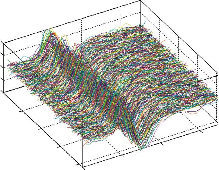
Neural basis of the BOLD fMRI signal N. K. Logothetis       1007

signal with the frequency content f. The gradient deter-              k space corresponding to different imaging techniques
mines a range of Larmor frequencies, and those fre-                   (Callaghan 1991). The scheme used is very often a zigzag
quencies can in turn provide exact position information.              pattern, scanning even and odd lines from left to right and
This is the trick. In an actual MRI sequence there are a              vice versa. The TE is defined here as the time from the
couple of basic elements for encoding the spatial infor-              excitation pulse to the centre of the k space. EPI can
mation, i.e. gradient schemes for slice selection (Gss), fre-         acquire images within a very short time (less than 50 ms)
quency encoding (readout) (Gro), and phase encoding                   and does so with a short TR to the order of 100 ms. Its
(Gpe). Here, we arbitrarily assign the directions x, y and            correct implementation, however, demands careful tuning
z to the readout (frequency encoding), phase encoding                 of sequence parameters to minimize image artefacts.
and slice-selection gradient directions (ro, pe and ss,
respectively).                                                        (iv) Image quality
   Figure 2 shows a typical pulsing diagram for a spin-echo              Image quality is determined by a number of interde-
image (commonly referred to as the conventional spin-                 pendent variables, including the SNR, the CNR, and the
warp two-dimensional fast Fourier transform image). To                spatial resolution. The SNR and CNR are both functions
select a slice, a frequency-selective RF pulse is used in             of the relaxation times, the scan properties, such as flip
combination with a field gradient perpendicular to the                angle, interpulse delay times and the number of averages,
desired slice. Figure 3a shows a typical RF pulse (sinc               the quality factor of the resonant input circuit (see § 4b(i)),
function) used to excite the tissue and figure 3b shows the           the noise levels of the receiver, and the effective unit vol-
spin echoes measured by two different channels (90° out               ume. The latter is determined by the slice thickness d,
of phase) combined as complex numbers. Two further                    the number of phase-encoding steps Npe, the number of
orthogonal gradients are used to extract the spatial infor-           samples in the frequency-encoding direction Nro and the
mation within the slice. The ‘readout’ gradient is applied            FOV. For an FOV of dimensions DroDpe the volume size
at the same time as the MR data are actually acquired                 is given by
(‘read’), while the ‘phase-encode’ gradient encodes the
second dimension in the image plane. For an image with                    Dro Dpe
                                                                      d           ,
NroNpe pixels, Nro points are sampled with the same ‘read-                Nro Npe
out’ gradient Gro, whereas for phase encoding the gradient            and the SNR by
Gpe is incremented Npe times. Thus, in each readout step,
the collected signal consists of the same frequencies dif-
                                                                      SNR ⬇
                                                                                dDroDpe
                                                                                             冑NEX,
fering only in their phases as determined by each phase-                        冑N     Npe
                                                                                      ro
encoding step. The acquired NroNpe data matrix,
usually termed the k space (figure 3c), with                          where NEX is the number of excitations (or averages).
kro,pe,ss = ␥ 兰 Gro,pe,ssdt, represents the image in the inverse      SNR also depends on the sampling frequency bandwidth;
spatial domain. Performing a Fourier transform for each               reducing the bandwidth increases SNR at the cost of
row extracts the amplitudes (figure 3d ), and performing it           increased sampling time. The maximum achievable SNR
for each column extracts the phase angles of the frequency            is of course determined to a significant extent by the
components (figure 3e). The amplitude of the central                  strength of the static magnetic field, B0. Increasing the
point of the k space determines the SNR of the global                 field strengthens the MR signal in an approximately linear
image. Sampling a larger number of points farther and                 fashion. In practice, the SNR and CNR can be estimated
farther away from the k space centre encodes the image’s              by measuring the signal of a tissue region or the signal
details and increases image resolution.                               difference between two different tissue regions and
   In many MRI methods, the acquisition of each row of                expressing that signal in units of the standard deviation of
the k space is preceded by an RF excitation. The pulse                the background signal (noise).
TR is dictated by the rate of recovery of longitudinal mag-              Spatial resolution is the smallest resolvable distance
netization, and the phase-encoding steps are determined               between two different image features. In the field of
by the desired resolution. Decreasing either one will affect          optics, it is usually determined on the basis of the Rayleigh
the image quality. This makes high-quality conventional               criterion, wherein objects can be distinguished when the
imaging too slow for comparing the MRI signal with its                maximal intensity of one occurs at the first diffraction
underlying neural activity. EPI (Mansfield 1977) permits              minimum of the other. An analogous expression of this
substantially faster data acquisition, and this is the                criterion which is directly applicable to MRI is that
approach currently being used in most rapid imaging                   between two maxima the intensity must drop below 81%
experiments and the one used in the studies described                 of its maximum value. Nominally, the spatial resolution
here (for a comprehensive review on EPI see Schmitt et                of an MR image is determined by the size of the image
al. (1998)). With EPI, an entire image can be created fol-            elements (voxels), that in turn is defined as the volume
lowing a single excitatory pulse because it collects the              covered (FOV) divided by the image points sampled dur-
complete dataset within the short time that the FID signal            ing acquisition (Rnom = FOV/N). In other words, voxel size
is detectable, that is, within a time for most applications           is defined by the slice thickness, the number of samples
limited by T ∗2 . Refocusing in EPI is achieved by the gradi-         in the phase and frequency-encoding directions, and the
ent (‘gradient echo’) rather than RF pulses. Along the                FOV. The optimal selection of voxel size is important.
readout direction an oscillating gradient permits the gen-            Large voxels will inevitably average the signal from the
eration of a train of echoes. Along the phase-encoding                tissue with functional variations across space. The smear-
direction, short blips advance the encoding to the next k             ing of local information acquired with large voxels—usu-
space line. There are many different ways of sampling the             ally termed the partial volume effect—alters both the

Phil. Trans. R. Soc. Lond. B (2002)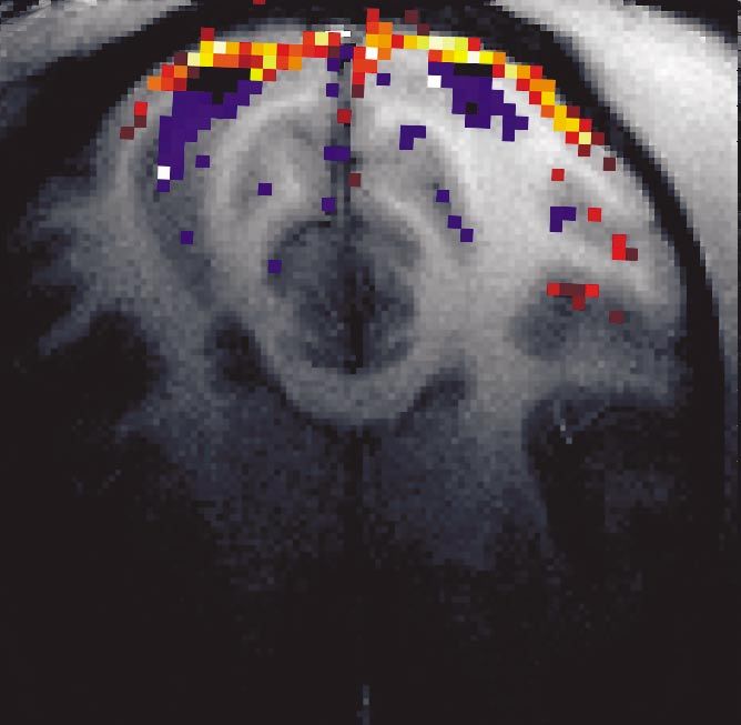
1008 N. K. Logothetis Neural basis of the BOLD fMRI signal

                                      90˚                     180˚

            RF pulse

            slice-
         selection Gz
          gradient

            phase-
         encoding Gy
          gradient

                                                            TE
       frequency-
                     readout
         encoding Gx
          gradient                                                                                    spin-echo

                                                                   TR
                                       preparation                                  sampling                 recovery

Figure 2. A highly simplified pulse sequence timing diagram. The actual pulse sequences have a number of additional
compensatory gradients used to negate the dephasing caused by the slice-selection and frequency-encoding gradients. For the
sake of simplicity no such additional pulses are displayed here. The pulse sequence is composed of three distinct phases: (i)
the preparation of transverse magnetization; (ii) the actual data collection (sampling); and (iii) sufficient recovery of the
longitudinal magnetization before the next repetition starts. In the first phase, the slice-selecting gradient (Gz) is turned on
during the 90° RF pulse. The phase-encoding gradient (Gy) turns on as soon as the RF activity ceases. The spatial location of
the spins along this gradient is again encoded by their frequency. But when the gradient is turned off all spins return to
uniform frequency, and the spatial information is only preserved in the form of their phase angles, which remain different
according to their location along the y-axis (hence the phase-encoding direction). Obviously the measured phase is the
vectorial sum of all phases along the y direction. Individual phases (encoding spatial location) can be only recovered by
applying phase-encoding pulses of different amplitudes during each repetition, depicted here as multiple polygons. The second
RF pulse (180°) combined with a second slice-selection gradient inverts the phase of the transverse magnetization and thus
generates a spin echo after time TE/2. Finally, a third gradient is used to create the positional dependence of frequency during
the collection of the spin echo. TE, echo time; TR, repetition time. Gz, Gy and Gx, the slice, phase-encoding and frequency-
encoding gradients, respectively.

waveform of the haemodynamic response and the frac-                     been developed over the last few decades to achieve this,
tional change in the MR signal. Reducing the voxel size,                ranging from simple surface coils (Ackerman et al. 1980)
however, while reducing the partial volume effects, affects             to quadrature coil combinations (Hyde et al. 1987) and a
both the SNR and the CNR of the image, thus imposing                    phased array of several coil loops (Roemer et al. 1990).
strong limitations on the image quality. Such limitations               Further improvement of sensitivity can be obtained by
can be minimized using stronger magnetic fields and                     using implantable, directly or inductively coupled RF coils
smaller RF coils.                                                       (see § 3).
   The nominal resolution of an image can be improved
by Fourier interpolation (or the mathematically equivalent
                                                                           3. FUNCTIONAL MRI WITH BOLD CONTRAST
‘zero filling’ in k space). Typically, signals acquired with
a resolution of NroNpe can be reconstructed as 2Nro2Npe                    MRI, like PET, can be used to map activated brain
images. This improves digital resolution by making                      regions by exploiting the well-established interrelation
implicit information visible to the viewer, but does not                between physiological function, energy metabolism and
change the spatial response function of the imaging                     localized blood supply. Different techniques can be
method or the image resolution according to the Ray-                    employed to measure different aspects of the haemody-
leigh criterion.                                                        namic response. For example, blood-supply changes can
   Like the SNR and CNR, the spatial resolution of an                   be used in perfusion-based fMRI, that measures blood
MR image depends on a number of scan factors, including                 flow quantitatively. Here, I shall concentrate on a single
gradient strength, sampling frequency bandwidth, recon-                 technique exploiting the BOLD contrast which, because
struction method and measurement sensitivity. All other                 of its reasonably high sensitivity and wide accessibility, is
factors being optimized, the last can be greatly improved               the mainstay of brain fMRI studies.
by closely matching the size, shape and proximity of an RF                 The BOLD contrast mechanism was first described by
coil to the structure of interest, a strategy that substantially        Ogawa et al. (1990a,b) and Ogawa & Lee (1990) in rat
improves the SNR of the image by decreasing the noise                   brain studies with strong magnetic fields (7 and 8.4 T).
detected by the coil. A number of different coil types have             Ogawa noticed that the contrast of very high resolution

Phil. Trans. R. Soc. Lond. B (2002)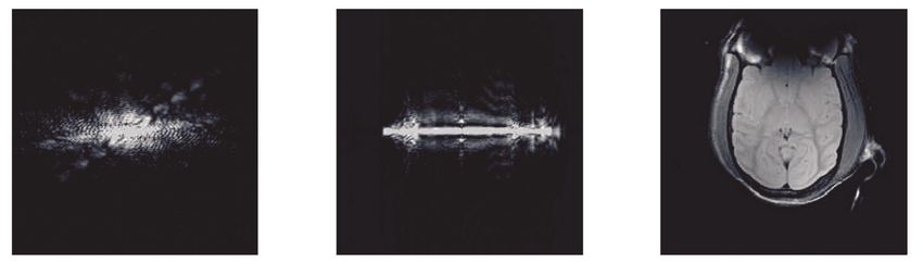
Neural basis of the BOLD fMRI signal N. K. Logothetis 1009
(a) (b)
1 1
chan 1 (real)
not actual 0.5
0.5 frequency
0
normalized amplitude
normalized amplitude
_0.5
0
chan 2 (imaginary)
0.5
_0.5 0
_0.5
_1 _1
_1.5 _1 _0.5 0 0.5 1 1.5 0.4 0.6 0.8 1.0 1.2 1.4 1.6
time (ms)
(c) (d) (e)
Figure 3. Image formation. (a) A typical RF excitation pulse (here sinc(x) = sin(x)/x) used to nutate the net magnetization
down into the xy plane. The RF pulse actually consists of the product of a sine wave of the Larmor frequency with the sinc
function. In the 4.7 T magnet this is ca. 200 MHz. The blue line depicts the sine wave at much lower frequencies for
illustration purposes. ␥ = 42.57 MHz T⫺1; resonance frequency = 200 MHz; duration = 3 ms; BW = 1.85 kHz. (b) The two spin
echoes produced by an inversion pulse of 180° (see also figure 2). In MRI the initially very high RF signal (MHz range) is
typically converted into an audio signal (kHz range) by comparing the RF signal with a reference signal (phase-sensitive
detection). In fact, to improve SNR the signal is collected by two PSDs that are 90° out of phase (upper and lower panels of
(b)). The converted signal is digitized and the two channels are represented as the real and imaginary part of complex
numbers (alternatively they can be transformed into the magnitude and phase of the signal). Each row of the k space consists
of a sequence of such numbers. TE = 15 ms; duration = 3 ms. (c) Magnitude of the k space in a spin-echo experiment. Each
row is an echo with the same frequency composition but different phase encoding. Top and bottom rows have the strongest
phase-encoding gradient and hence the largest dephasing (weakest signal). The strongest echo is in the centre of the k space,
where no phase-encoding occurs. (d ) The first Fourier transformation along the readout direction. (e) The second Fourier
transformation along the phase-encoding direction resulting in the actual image.
images (65 × 65 × 700 m3) acquired with a gradient– The paramagnetic nature of dHb (Pauling & Coryell
echo–pulse sequence depicts anatomical details of the 1936) and its influence on the MR signal (Brooks et al.
brain as numerous dark lines of varying thickness. These 1975) were well known before the development of MRI.
lines could not be seen when the usual spin-echo Haemoglobin consists of two pairs of polypeptide chains
sequences were used, and they turned out to be image (globin), each of which is attached to a complex of proto-
‘artefacts’, signal dropouts from blood vessels (Ogawa et porphyrin and iron (haem group). In dHb the iron (Fe2⫹)
al. 1990a). In other words, by accentuating the suscepti- is in a paramagnetic high-spin state, as four of its six outer
bility effects of dHb in the venous blood with gradient– electrons are unpaired and act as an exogenous paramag-
echo techniques, Ogawa discovered a contrast mechanism netic agent. When oxygenated, the haem iron changes to
reflecting the blood oxygen level, and realized the poten- a low-spin state by receiving the oxygen’s electrons.
tial importance of its application by concluding that The magnetic properties of dHb would be of little value
‘BOLD contrast adds an additional feature to magnetic if haemoglobin were evenly distributed in all the tissues.
resonance imaging and complements other techniques Instead, paramagnetic dHb is confined in the intracellular
that are attempting to provide PET-like measurements space of the red blood cells that in turn are restricted to
related to regional neural activity’ (Ogawa et al. 1990b). the blood vessels. Magnetic susceptibility differences
Shortly after this, the effect was nicely demonstrated in between the dHb-containing compartments and the sur-
the cat brain during the course of anoxia (Turner et al. rounding space generate magnetic field gradients across
1991). As is now known, the phenomenon is indeed due and near the compartment boundaries. Pulse sequences
to the field inhomogeneities induced by the endogenous designed to be highly sensitive to such susceptibility differ-
MRI contrast agent dHb. ences, like those used by Ogawa in his seminal studies
Phil. Trans. R. Soc. Lond. B (2002)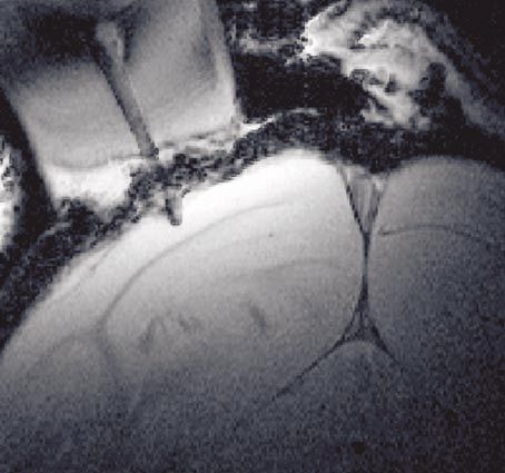
1010 N. K. Logothetis Neural basis of the BOLD fMRI signal
(Ogawa & Lee 1990; Ogawa et al. 1990a,b), generate (i) long-range interactions between different brain
signal alterations whenever the concentration of dHb structures;
changes. The field inhomogeneities induced by dHb mean (ii) task- and learning-related neurochemical changes by
that neural activity should result in a BOLD signal means of localized in vivo spectroscopy or MRS
reduction. However, during brain activation the BOLD imaging;
signal increases rather than decreasing relative to a resting (iii) dynamic changes in the magnitude and location of
level. This is because activation within a region causes an activated regions—over periods of minutes to days—
increase in CBF and the use of glucose, but not a com- with priming, learning and habituation;
mensurate increase in the oxygen consumption rate (iv) dynamic connectivity patterns by means of labelling
(Fox & Raichle 1986; Fox et al. 1988). This results in a techniques involving MR contrast agents; and
decreased oxygen extraction fraction and lower dHb con- (v) plasticity and reorganization following experimen-
tent per volume unit of brain tissue. tally placed focal lesions.
Not surprisingly, the groundbreaking work of Ogawa
excited great interest in the application of BOLD fMRI to In addition, the application of this technique to the
humans. MR-based CBV imaging had already been dem- behaviour of monkeys has the potential to build a bridge
onstrated in humans using high-speed EPI techniques and between human studies and the large body of animal
the exogenous paramagnetic contrast agent gadolinium research carried out over the last 50 years.
(Belliveau et al. 1991; Rosen et al. 1991). In 1992, how- Monkeys are ideal experimental animals because a great
ever, three groups simultaneously and independently deal is known about the organization of their sensory sys-
obtained results in humans with the BOLD mechanism tems that are functionally very similar to those of humans.
(Bandettini et al. 1992; Kwong et al. 1992; Ogawa et al. In addition, comparisons of psychophysical data from
1992), starting the flood of fMRI publications that have humans and the most commonly used species, the rhesus
been appearing in scientific journals ever since. macaque, have revealed remarkable behavioural simi-
Research over the last decade has established that larities between the two species. Thus, MRI in monkeys
BOLD contrast depends not only on blood oxygenation not only provides insights into the neural origin of the
but also on CBF and CBV, representing a complex fMRI signals, but it can do so in the context of different
response controlled by several parameters (Ogawa et al. types of behaviour. With this conviction, we set out to
1993, 1998; Weisskoff et al. 1994; Kennan et al. 1994; develop and apply MRI (and MRS) in monkeys, using
Boxerman et al. 1995a,b; Buxton & Frank 1997; Van Zijl both conventional volume coils for whole-head scanning
et al. 1998). Despite this complexity, much progress has and implanted coils allowing imaging with high spatial
been made toward quantitatively elucidating various resolution.
aspects of the BOLD signal and the way it relates to the Figure 4 shows the system used for imaging the monkey
haemodynamic and metabolic changes occurring in brain. It is a vertical 4.7 T scanner with a 40 cm diameter
response to elevated neuronal activity (Kim & Ugurbil bore (Biospec 47/40v; Bruker Medical Inc., Ettlingen,
1997; Buxton et al. 1998; Van Zijl et al. 1998). Germany). The scanner is equipped with a 50 mT m⫺1
BOLD fMRI has also been applied successfully in (180 s rise time) actively shielded gradient coil (Bruker,
anaesthetized or conscious animals, including rodents B-GA 26) of 26 cm inner diameter. A primate chair and
(Hsu et al. 1998; Lahti et al. 1998; Bock et al. 1998; Tuor a special transport system were designed and built to pos-
et al. 2000; Burke et al. 2000; Ances et al. 2000; Burke et ition the monkey inside the magnet (Logothetis et al.
al. 2000; Chang & Shyu 2001), rabbits (Wyrwicz et al. 1999). Whole-head scans were carried out with either lin-
2000), cats ( Jezzard et al. 1997), bats (Kamada et al. ear birdcage-type coils or with custom-made linear homo-
1999), and recently monkeys (Nakahara et al. 2002; Logo- geneous saddle coils. For high-resolution fMRI, we used
thetis et al. 1998, 1999; Disbrow et al. 1999; Zhang et al. customized small RF coils (see § 4b) which had been
2000; Disbrow et al. 2000; Vanduffel et al. 2001; Dubo- optimized for increased sensitivity over a given ROI
witz et al. 2001). What follows describes the use of BOLD (Logothetis et al. 2002). In the combined physiology and
fMRI in monkeys (Macaca mulatta) and its combination fMRI sessions (see § 5a), the coils were attached around
with electrophysiological measurements in an attempt to the recording chamber and were used as transceivers
investigate the neural basis of the BOLD response. (Logothetis et al. 2001).
(a) Large FOV imaging: volume coils
This section introduces a few applications with volume,
4. MRI OF THE MONKEY BRAIN whole-head coils that demonstrate the value of the tech-
nique for research involving:
fMRI and microelectrode recordings are complemen-
tary techniques, providing information on two different (i) the comparison of monkey and human sensory sys-
spatio-temporal scales. The electrodes have excellent spa- tems;
tio-temporal resolution but very poor coverage, while (ii) microelectrode recordings from different sites of dis-
fMRI has relatively poor resolution but can yield tributed neural networks subserving a behaviour
important information on a larger spatio-temporal scale. under investigation; or
The development and application of NMR techniques (iii) the planning of selective focal brain lesions in the
(e.g. imaging, spectroscopy) for the non-human primate context of investigations into behavioural disorders
enables the investigation of certain levels of neural organi- to illuminate the role of a particular brain region.
zation that cannot be studied by electrodes alone. These
include the study of: Details on these applications can be found in various
Phil. Trans. R. Soc. Lond. B (2002)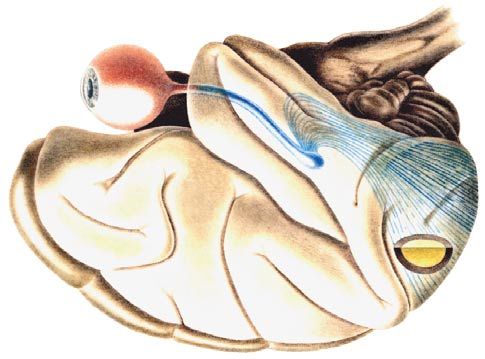
Neural basis of the BOLD fMRI signal N. K. Logothetis 1011
(eight segments) gradient-recalled EPI, with an FOV of
128 mm × 128 mm on a 128 × 128 matrix and a voxel size
of 1 mm × 1 mm × 2 mm.
(ii) Retinotopy
The robustness of activation and the spatial selectivity
of the BOLD signal can be examined by exploiting the
well-established retinotopic organization of the visual sys-
tem. In humans, retinotopy can be reliably demonstrated
in fMRI by using slowly moving, phase-encoded retino-
topic stimuli (Engel et al. 1994, 1997; Deyoe et al. 1994;
Sereno et al. 1995).
We have used the same approach to study the retinotop-
ical organization of the monkey visual areas. As in human
studies, the stimuli consisted of a series of slowly rotating
wedges or expanding rings, each wedge or ring being a
collection of flickering squares (Engel et al. 1994, 1997;
Wandell et al. 2000). The ring typically begins as a small
spot located at the centre of the visual field and then grows
until it travels beyond the edge of the stimulus display. As
it disappears from view, it is replaced by a new spot start-
ing at the centre. Such an expanding stimulus causes a
travelling wave of neural activity beginning a couple of
millimetres posterior to the lunate sulcus (figure 6a,b) and
travelling in the posterior direction toward the pole of the
occipital lobe. The temporal phase of the MRI signal var-
ies as a function of eccentricity, and this phase can be
used to generate the eccentricity maps shown in figure 6c
(adapted from Brewer et al. (2002)). This technique made
Figure 4. The scanner system. A vertical 4.7 T magnet with it possible to identify the boundaries between visual areas
a 40 cm diameter bore was used to image monkey brains. V1, V2, V3 and V4 and V5 (MT) and to measure the
The magnet has local passive shielding to permit the use of visual-field eccentricity functions that reveal the distri-
neurophysiology and anaesthesia equipment. It is equipped bution of foveal and peripheral signals within the ventral
with a 50 mT m⫺1 (180 s rise time) actively shielded and dorsal streams, respectively (Wandell et al. 2000;
gradient coil (Bruker, B-GA 26) with an inner diameter of
Brewer et al. 2002). The maps obtained in this manner
26 cm. A primate chair and a special transport system were
designed and built for positioning the monkey within the are in excellent agreement with those derived from mon-
magnet. keys with anatomical and physiological techniques, and
they can be used to study the process of cortical reorgani-
zation after deafferentiation (e.g. Kaas et al. 1990; Darian-
recent publications (Logothetis et al. 1999; Rainer et al. Smith & Gilbert 1995; Das & Gilbert 1995; Obata et al.
2001; Tolias et al. 2001; Brewer et al. 2002; Sereno et 1999). Such applications demonstrate the quality of data
al. 2002). that can be obtained in the monkey, and the feasibility
of a direct comparison between human and non-human
(i) Activation of the thalamus and visual cortex primate studies.
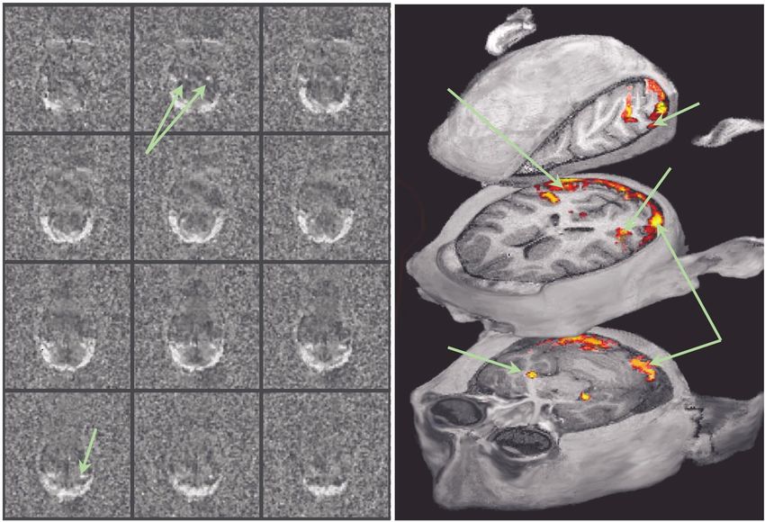
Figure 5 shows the results from a macaque monkey
scanned under isoflurane (0.4%) anaesthesia (Logothetis (b) High-spatial resolution imaging: surface coils
et al. 1999). The left half of the figure depicts typical z- Whole-head imaging, although of great importance for
score maps for 12 horizontal slices. No threshold was the localization of activations, is of limited value when very
applied to the statistical maps so that one can directly see high spatio-temporal resolution is required to study corti-
the strength of the difference signal and its relationship to cal microarchitecture or to compare imaging with electro-
noise. On the right half, thresholded z-score maps show- physiology. We have therefore adapted and optimized the
ing brain activation are colour coded and superimposed implanted coil technique for monkeys. Very high-
on anatomical scans as slices of the computer-rendered resolution structural and functional images of the monkey
monkey head. The activation was elicited by a polar-trans- brain were obtained with small, tissue-compatible, intra-
formed checkerboard pattern rotating in alternating direc- osteally implantable RF coils. Voxel sizes as small as
tions. 0.012 l (125 × 125 × 770 m3) were obtained with high
Figure 5a,b shows a robust BOLD signal in the LGN values of the SNR and CNR, revealing both structural and
as well as in the striate and extrastriate cortices. functional cortical architecture in great detail.
The anatomical scan was acquired with an FOV of
128 mm × 128 mm with a matrix of 256 × 256 and slice (i) Implanted RF coils
thickness of 0.5 mm using the three-dimensional MDEFT As mentioned in § 2b, the RF system is a transceiver
(Ugurbil et al. 1993) pulse sequence. The fMRI was car- system used both to generate the alternating B1 field and
ried out by multi-slice (13 slices, 2 mm thick), multi-shot to receive the RF signal transmitted by the tissue (for a
Phil. Trans. R. Soc. Lond. B (2002)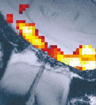
1012 N. K. Logothetis Neural basis of the BOLD fMRI signal
(b)
0 1 2
V2
V4
3 4 5
LGN V5 (MT)
6 7 8
LGN V1
9 10 11
V5 (MT)
Figure 5. (a) BOLD activation shown in terms of z-score maps. The specificity of the signal enables the visualization of
anatomical details in the occipital lobe. (b) Activation maps superimposed on anatomical three-dimensional MDEFT scans
(0.125 l voxel size). The figure shows activation of the LGN, striate and some extrastriate areas including V2, V3, V4 and
V5 (MT). V1 activation covers almost the entire representation of the perifovea (the horizontal extent of the checkerboard
stimulus was 30°). The V1 regions showing high activation (yellow) lie within the cortical representation of the fovea.
review on principles and instrumentation see Vlaardinger- 1987; Garwood et al. 1989; Gruetter et al. 1990; Walker et
broek & Den 1996; Wood & Wehrli 1999; Matwiyoff & al. 1991; Merkle et al. 1993; Hendrich et al. 1994; Lopez-
Brooks 1999). It is typically an integral part of any imaging Villegas et al. 1996). The SNR of such coils can be further
system, and is delivered with the magnet and all the other increased by geometrically matching the coil to a specific
components of a scanner. However, coils can also be cus- tissue region. Finally, in animal experiments, the SNR can
tom made in all kinds of different designs to accommodate be substantially increased by implanting the coils in the
the needs of specific experiments. They can be used as body (Farmer et al. 1990; Summers et al. 1995; Silver et
transceivers, but also as transmit- or receive-only units, al. 2001). Implanted coils bring about a substantial
the former transmitting the B1 field and the latter receiving increase in both the SNR and spatial selectivity by effec-
the FID after an adjustable delay. tively improving the filling factor of a reception coil. The
Technically, RF coils are equivalent to an electrical cir- measured signal typically decreases as the distance of the
cuit with inductance (L), capacitance (C) and resistance coil from the ROI increases, while the noise detected by
(R), and are tuned to a specific resonance frequency () a coil increases with coil size. Thus, the smaller the coils
(e.g. 200 MHz at 4.7 T); for MRI this is the precessional and the closer the area of interest, the better the
frequency of the nuclear spin moments. Optimizing a coil obtained signal.
commonly involves increasing its quality factor (or filling The small RF surface coils described here were
factor), Q. The latter is defined as the maximum energy
implanted intraosteally. They were made of 2 mm thick,
stored divided by the average energy dissipated per radian,
Teflon-insulated, fine silver wire and had diameters vary-
and can be improved by fine tuning the parameters L and
ing from 18 to 30 mm. The implantable coils were 15 or
C and minimizing R (the smaller the resistance, the
22 mm in diameter (see figure 7). Their electronic cir-
sharper the resonance curve) for any given frequency. The
cuitry had non-magnetic (copper–beryllium) slotted tubes
RF coil design can be optimized (i) for signal homogeneity
to ensure a reliable electrical connection. During the sur-
over the whole brain, (ii) for increased sensitivity over a
gical placement of the implanted coils, special care was
given ROI, an example being the large quadrature surface
coils, or (iii) for very high-resolution studies of a small taken to optimize the loaded Q of the coils. The Q factor
area of interest (surface coils). can be directly affected by placing the coil too far from—
Small surface coils are often used in either human or but also too close to—the ROI. The appropriate distance
animal studies to provide the highest possible SNR and of the coil from the ROI was therefore calculated based
to allow the use of small voxel sizes in high-resolution on models of the brain and skull surfaces created from
imaging (e.g. McArdle et al. 1986; Le et al. 1987; Rudin anatomical scans.
Phil. Trans. R. Soc. Lond. B (2002)Neural basis of the BOLD fMRI signal N. K. Logothetis 1013
(a) (b)
po
lu
HM
F
la io
UVM
sts
(c)
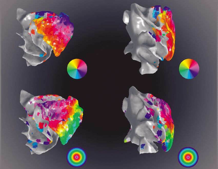
Figure 6. Retinotopic organization revealed with fMRI. (a) Lateral view of a computer-rendered monkey brain. It shows some
of the primary sulci. (b) Latero-caudal view of the posterior part of the brain with opened-up sulci. It shows the fovea and the
horizontal and vertical meridians as determined with phase-encoding stimuli. (c) The upper panels show the eccentricity maps
and the lower panels the orientation maps generated by using expanding-ring and rotated-wedge stimuli, respectively.
Abbreviations: la, lateral; sts, superior temporal; io, inferotemporal, lu, lunate; po, parieto-occipital; HM, horizontal meridian;
UVM, upper vertical meridian; F, foveal representation.
(ii) High-resolution echo-planar BOLD imaging etration. Cortical vessels, that were traditionally divided
Figure 8 shows anatomical and functional scans into three groups (short, intermediate and long), were
acquired with an implanted surface coil. Figure 8a is an further divided by Duvernoy et al. (1981) into six groups
example of a T∗2 -weighted echo planar (EP) image according to their length and termination in the various
obtained with an actual resolution of 125 × 125 m2 and cortical layers. The green arrows show two vessels of
a slice thickness of 720 m. The contrast sensitivity of the Group 5 according to Duvernoy et al. (1981) consisting
image is sufficient to reveal the characteristic striation of of arteries and veins (the MR images show the veins) that
the primary visual cortex. The dark line shown by the pass through the entire cortical thickness and vascularize
white arrow (Gen) is the well-known, ca. 200 m thick both cortex and the adjacent WM (figure 5c,d). Measure-
Gennari line between the cortical layers IVA and IVC, a ments after methyl methacrylate injections show that the
result of the axonal plexus formed by the axons of pyrami- veins of this group have an average diameter of 120 m.
dal and spiny stellate cells contained in IVB. It appears The actual resolution of the presented image permits the
dark in T ∗2 -weighted images because the plexus contains visualization of susceptibility effects produced by such
a large number of horizontally arranged, myelinated (the tiny vessels.
T2-values are shorter for fat; see § 2b(ii)) axons from col- Figure 8e shows fMRI correlation coefficient maps (in
laterals, horizontal axonal branches, and ascending rami- colour) superimposed on the actual EPI (T∗2 -weighted)
fications of spiny stellates. images of a monkey during visual block-design stimu-
Also visible in figure 8b are the small cortical blood ves- lation. The sections are around the lunate sulcus, and acti-
sels that are known to vary in their degree of cortical pen- vation extends into the primary and secondary visual
Phil. Trans. R. Soc. Lond. B (2002)1014 N. K. Logothetis Neural basis of the BOLD fMRI signal
lead to signal enhancement in the image of a selected slice
if the time between consecutive RF excitations is insuf-
ficient for the signal within the slice to reach full relax-
ation. Such inflow effects can be considerably stronger
than the BOLD signal itself (Segebarth et al. 1994; Frahm
et al. 1994; Kim et al. 1994; Belle et al. 1995) and much
less tissue specific. The shorter the repetition times, the
stronger the inflow effect will be (Glover & Lee 1995;
Haacke et al. 1995). Inflow effects can be eliminated by
utilizing low flip angles and increasing the TR time
(Menon et al. 1993; Frahm et al. 1994).
Assuming the appropriate selection of pulsing para-
meters to minimize the above-mentioned effects, the issue
of spatial specificity can be addressed by conducting spe-
cific experiments targeted at mapping functionally distinct
Figure 7. Implantable RF coils. The coils were made of structures with well-defined organization and topography
insulated silver wire and were used either as transceivers or in the brain. The activation of LGN shown in figure 5 is
receive-only units. All circuits were equipped with non- an example of such specificity, as the structure is only ca.
magnetic (copper–beryllium) slotted tubes to ensure reliable 6 mm in the rostrocaudal, and ca. 5 mm in the dorsoven-
connection with the silver-wire loops.
tral and mediolateral directions.
Figure 9 demonstrates the spatial specificity of BOLD
cortices (V1 and V2, respectively). The images have high by exploiting the non-uniform distribution of directionally
SNR (27:1 for an ROI of 36 voxels, measured for an ROI selective cells across the layers of the striate cortex. About
positioned over the high-signal-intensity region in the one-third of the striate cells are known to be directionally
image) and CNR (21:1 and signal modulation ranging selective (Goldberg & Wurtz 1972; Schiller et al. 1976;
from 2 to 7%, averaged for ROI of ca. 15–24 voxels). Both De Valois et al. 1982; Albright 1984; Desimone & Unger-
robust activation and good anatomical detail can be dis- leider 1986; Colby et al. 1993). However, these cells do
cerned. not exhibit a uniform laminar distribution. Instead, most
are found in layers 4A, 4B, 4C␣ and 6 (Dow 1974;
(iii) Spatial specificity of BOLD fMRI Hawken et al. 1988). In high-field MRI such differences in
Gradient echo sequences like those used extensively for neuron density can be visualized if the appropriate visual
BOLD imaging are sensitive to both small and large ves- stimuli are used and the pulsing parameters are tuned to
sels (Weisskoff et al. 1994). The significant contribution stress the extravascular BOLD signals. Figure 6a,b shows
of the large vessels can lead to erroneous mapping of the the z-score maps obtained by comparing the activation
activation site, as the flowing blood will generate BOLD elicited by the moving checkerboard stimulus to that elic-
contrast downstream of the actual tissue with increased ited by the blank screen and the counter-flickering
metabolic activity. Thus, the extent of activation will checkerboard stimulus, respectively (Logothetis et al.
appear to be larger that it really is. The contribution of 2002). The parameters used in this scan were:
large vessels depends on both field strength and the para- FOV = 32 mm × 32 mm on a matrix of 256 × 256 voxels
meters of the pulse sequences (Boxerman et al. 1995a; (0.125 mm × 0.125 mm resolution), slice thickness =
Zhong et al. 1998; Hoogenraad et al. 2001). 1 mm, TE/TR = 20/750 ms, and number of segments = 8.
Large vessels can be de-emphasized using pulse Figure 9c illustrates the plane of the slice selected for high-
sequences designed to suppress higher flow velocities resolution imaging and figure 7d illustrates the signal
(Boxerman et al. 1995a). They are also de-emphasized in modulation. For the most part, activity in V1 was found
stronger magnetic fields, because the strength of extra- in the middle layers, usually layer IV. This activity may
vascular BOLD increases more rapidly for small vessels indeed reflect the density of active directional neurons
than it does for large ones. More specifically, the trans- within this lamina. However, it is possible that the acti-
verse relaxation rate, R∗2 , increases linearly with the exter- vation in the middle layers of cortex reflects the highest
nal magnetic field for large vessels (larger than 10 m) but capillary density that occurs at approximately layers 3C,
varies as the square of the field for small vessels (Ogawa 4 and 5 (vascular layer 3 as defined by Duvernoy et al.
et al. 1993; Gati et al. 2000). Thus, with sufficient SNR, (1981)). A recent human fMRI study indicates that the
signals originating from the capillary bed are clearly dis- origin of the BOLD signal may actually be the vascular
cernible in strong magnetic fields. layer 3, presumably extending into adjacent vascular layers
A loss of specificity can also result from so-called inflow (Hyde et al. 2001). Further experimentation is needed to
effects. Both supplying pial arteries and draining vessels dissect the effect of vascular density from that of neural
unavoidably bring fresh spins into the area of interest dur- specificity.
ing the inter-image delay. For instance, when short rep-
etition times are used, gradient–echo sequences yield (c) High-temporal resolution imaging
considerable contrast between the partially saturated In order to compare imaging with physiology we used
tissues in the imaging plane, i.e. tissues whose longitudinal a rapid scanning protocol to acquire a single slice contain-
magnetization was not yet fully recovered, and the unsatu- ing the microelectrode tip (GR-EPI with four segments
rated blood flowing into this plane (Axel 1984, 1986). In and TE/TR = 20/250 ms). To minimize the effects of inflow
the same vein, increased CBF in an activated tissue will and large drainage vessels, we consistently used flip angles
Phil. Trans. R. Soc. Lond. B (2002)You can also read