The relation between supply constraints and house price dynamics in the Netherlands - No. 601 / July 2018 - Dnb
←
→
Page content transcription
If your browser does not render page correctly, please read the page content below
No. 601 / July 2018

The relation between supply constraints
and house price dynamics in the
Netherlands
Bahar Öztürk, Dorinth van Dijk, Frank van Hoenselaar and Sander Burgers
The relation between supply constraints and house price
dynamics in the Netherlands
Bahar Öztürk, Dorinth van Dijk, Frank van Hoenselaar and Sander Burgers *

* Views expressed are those of the authors and do not necessarily reflect official positions
of De Nederlandsche Bank.

                                                                De Nederlandsche Bank NV
Working Paper No. 601                                           P.O. Box 98
                                                                1000 AB AMSTERDAM
July 2018                                                       The Netherlands
The relation between supply constraints and house price dynamics in
the Netherlands∗
Bahar Öztürka, Dorinth van Dijka,b, Frank van Hoenselaara, and Sander Burgersb
a
De Nederlandsche Bank, the Netherlands
b
University of Amsterdam, the Netherlands
16 July 2018
Abstract
We analyze the effect of supply constraints on the dynamics of house prices in the Netherlands. In
particular, we look at whether income shocks lead to stronger house price increases in regions
characterized with higher supply constraints. We use a panel dataset that contains 316
municipalities over the years 1987-2016. Municipalities are divided in three equally sized groups
according to the extent of supply constraints present in each municipality. Our results suggest that
income shocks lead to significantly larger increases in house prices in municipalities that are
relatively more supply constrained. This holds both in the short- and the long-term. The degree of
mean reversion and persistence, however, do not seem to significantly differ between the three
groups of municipalities.
Keywords: house prices, income shocks, supply constraints
JEL classifications: G120, R310.
∗
Corresponding authors: Bahar Öztürk (b.ozturk@dnb.nl) and Frank van Hoenselaar (f.j.g.van.hoenselaar@dnb.nl ). We are grateful to
Maurice Bun, Jakob de Haan, Jante Parlevliet, Peter van Els, Maarten van Rooij, and Johan Verbruggen for useful comments on earlier
versions. Views expressed do not necessarily reflect those of De Nederlandsche Bank.
11. Introduction
After having sharply declined during the Great Financial Crisis, house prices in the Netherlands
have been increasing strongly since 2014. There is substantial heterogeneity between regions,
however. Nominal house prices in Amsterdam stood in 2018Q1 32% above their pre-crisis peak of
2008Q3, whereas in the more rural province of Friesland they were 8% below their pre-crisis peak.
Due to the relevance of house price swings for macroeconomic stability and the existence of
spillover effects between regions (Vansteenkiste, 2007; Teye & Ahelegbey, 2017), it is of great
importance for policymakers to gain a good understanding of the heterogeneity in house price
developments across regions and the drivers of this heterogeneity.
A typical feature of the Dutch housing market is that the price elasticity of housing supply is low,
which is partly related to the relatively high population density (Caldera & Johansson, 2013).
Moreover, the supply elasticity is generally lower in the major cities compared to the rest of the
country (Michielsen et al., 2017). If housing supply inadequately adjusts to changes in housing
demand, this might lead to house prices deviating from their equilibrium values for an extended
period of time (Capozza, 2002). In the literature, a low supply elasticity is often linked to physical
supply constraints related to geography (Saiz, 2010) or a rigid planning system (Hilber &
Vermeulen, 2016). For the Netherlands, both sources of supply restrictions are relevant. In various,
mostly urban areas, new construction is restricted because a considerable share of land is already
developed (physical constraints). In addition, new housing supply is further hampered by a planning
system that is fairly restrictive (Rouwendal & Vermeulen, 2007). In this paper, we look at supply
constraints as a whole as we are not able to distinguish between physical and regulatory constraints
due to lack of data on the rigidity of the planning system. However, physical and regulatory supply
constraints are highly correlated in practice (Saiz, 2010).
This paper studies the effect of supply constraints on the dynamics of house prices in the
Netherlands. In particular, the hypothesis is that a shock in real household income will have a
stronger effect on house prices in municipalities with stronger supply constraints. Based on the
methodology developed by Hilber & Vermeulen (2016), we create an index for the extent of supply
constraints in a given region (i.e. municipality) by relating the amount of already developed land
to total available developable land. Based on this variable, we divide the sample into three equally-
sized groups of municipalities: municipalities with low, medium, and high supply constraints,
labeled as “least developed”, “medium developed” and “most developed”, respectively. We then
2study the relation between house prices and income shocks, using a two-step Engle and Granger
approach. Our results suggest that income shocks are associated with significantly larger increases
in house prices in municipalities that face relatively strong supply constraints.
The rest of the paper is structured as follows. In section 2, we briefly discuss how the existing
literature is related to our work. In section 3, we elaborate on our measure of supply constraints.
Section 4 first describes the data and the methodology used in the empirical analysis, and then
discusses the results. Section 5 concludes.
2. Related literature
Our work is closely related to a large body of literature that discusses the fundamental factors
driving house prices (see for instance Capozza et al., 1989, 2002). Empirical studies find that real
income, real interest rates and real construction costs consistently prove to be important
determinants of long-run house prices (see among others Abraham & Hendershott, 1994). In
addition, several studies consider a number of additional variables that appear to also significantly
explain the equilibrium house prices such as household wealth, rental prices, population and the
housing stock (see, for instance, Kranendonk et al., 2005).
It is often found that regions where housing supply is more restricted due to geographical and/or
regulatory constraints exhibit different house price dynamics. These constraints tend to lower the
elasticity of housing supply significantly, preventing new housing supply to exert downward
pressure on prices (Green et al., 2005). Glaeser et al. (2008) show that areas with stronger supply
constraints in the United States, e.g. San Francisco Bay Area, experienced a larger housing boom
in the 1982-2007 period. Extending on this research, Huang & Tang (2012) find furthermore that
these areas also experienced larger housing busts during the recent global financial crisis. This
finding might seem counterintuitive as one might reason that limited construction during a boom
phase could also result in a limited downward pressure during a bust period. However, as Huang
and Tang argue, during a boom phase the adaptive expectations of those who aspire to buy a house
lead to overshooting of prices in the more supply-constrained areas, exacerbating the busts that are
due to follow. Heebøll & Anundsen (2016) argue further that besides adaptive expectations, the
financial accelerator effect is also more pronounced in more restricted areas. As a result, increasing
(decreasing) house prices lead to more (less) optimistic beliefs on future house prices and more
(less) collateral to borrow against. Hilber & Vermeulen (2016) find that regulatory constraints
3induced by the UK planning system, significantly increased house prices and house price volatility
in the most constrained areas in the 1974 - 2008 period. Finally, Capozza et al. (2002), the closest
work to our paper, analyzes house price dynamics in various US metropolitan areas and find that
areas that face stronger supply constraints also experience stronger serial correlation (i.e.
persistence in house price growth) and slower mean reversion of prices (i.e. the speed of adjustment
to the long-run equilibrium house price).
The goal of this paper is to study the interaction of supply constraints with house price dynamics
in the Netherlands. A well-known measure of supply constraints is developed by Saiz (2010), who
measures physical supply constraints in the United States by making use of elevation in the
landscape. This measure, however, is not suitable for our study as the variation in elevation levels
is very low in the Netherlands. Instead, we use the measure developed by Hilber & Vermeulen
(2016), i.e. the share of already developed land of total developable land, which is discussed in
more detail in Section 3. It is important to note that physical and regulatory supply constraints are
highly correlated in practice (Saiz, 2010), and what we observe here as supply constraints is driven
by both physical and regulatory constraints.
A few papers have studied the (heterogeneous) price dynamics of the Dutch housing market.
Kranendonk et al. (2005) have estimated an error-correction model for the 1980-2003 period and
found that house prices tend to adjust to the equilibrium price much more quickly when house
prices are below their equilibrium value than when they are above. Galati et al. (2011) study the
price dynamics in various Dutch housing markets and conclude that mean reversion is the lowest
in the most urbanized areas. This finding seems to be in line with the findings of Capozza et al.
(2002), assuming that more urbanized (i.e. more densely populated) areas are also more supply-
constrained. However, in a somewhat more recent study Galati & Teppa (2017) come to a different
conclusion and find that mean reversion is lowest in both the least and most urbanized segments of
the Dutch housing market.
The contribution of our study to this literature is twofold. First, we employ a rich dataset that allows
us to study the short- and long-run dynamics of house prices at a more granular level (municipality)
than previous work on the Dutch housing market. Second, we add to the existing literature by
studying the interaction between income shocks and housing supply constraints.
43. A measure for supply constraints in the Netherlands
In order to determine the extent of supply constraints, we apply the methodology of Hilber &
Vermeulen (2016) to the Netherlands. More specifically, we calculate the ratio of developed land
to developable land. We use the Dutch land cover map (Het Landelijk Grondgebruiksbestand
Nederland, LGN5) as data source. LGN5 is a 25x25m raster file that contains data on 39 different
land uses based on satellite images and aerial photos from 2003 and 2004. The database is created
and updated by Wageningen University. Although the classification of land uses in the Netherlands
is somewhat different compared to that in the United Kingdom, we follow Hilber & Vermeulen
(2016) as closely as possible and categorize the classifications into developed land, developable
land and non-developable land. The classification between developable and non-developable is
sometimes somewhat arbitrary, but new development in the developable category is arguably
somewhat easier. Technically all land types, even water in the Netherlands (e.g. De Flevopolder
was converted from water into land between 1950 and 1968), can be converted into developed land
in the (very) long-run. Besides, the main driver behind the measure is the amount of developed land
since share of non-developable land is usually rather small.
As developed land we classify the land uses ’urban developed’, ’suburban developed’, ’densely
developed in forest’, ’roads and railroads’, and ’rural developed’. In developable land we include
’grass’, ’corn fields’, ’strawberry fields’, ’beet fields’, ’grain fields’, ’other fields’, ’greenhouse’,
’orchard’, ’bulb fields’, ’deciduous woodland’, coniferous woodland’, ’deciduous woodland in
developed area’, ’coniferous woodland in developed area’, ’grass in developed area’, ’inland bare
ground’, ’heath’, ’medium grassed heath’, ’strongly grassed heath’, ’peat moor’, ’peat moor
woodland’, ’swamp’, ’reed vegetation’, ’forest in swamp’, ’peatland’, ’natural reserve’, and ’inland
bare ground in natural reserve’. Finally, in non-developable land we include ’salt water’, ’sweet
water’, ’saltmarsh’, ’costal bare ground’, ’open dune vegetation’, ’closed dune vegetation’, ’dune
heath’, and ’open drift-sand’.
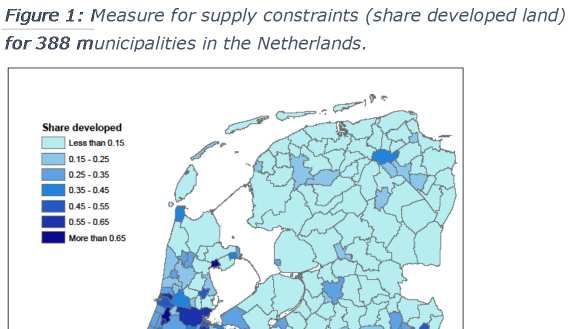
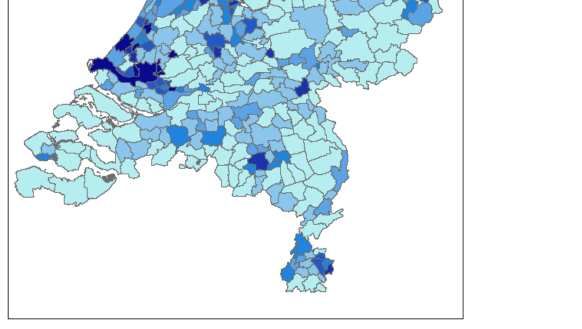
The share of developed land (termed as “share developed” below) is the amount of developed land
divided by the total amount of developable land (already developed and potentially developable).
As geographical borders, we use the municipal borders according to the municipal definition of
2017. The share developed land is calculated for a total of 388 municipalities and is included in
Figure 1. As expected, we clearly observe that large cities like Amsterdam, Rotterdam, The Hague,
and Utrecht are relatively densely developed compared to more rural areas around Friesland and
5Groningen. The average share developed is 0.21, ranging from 0.03 (Rozendaal) to 0.75 (Leiden).
The value of the four largest cities are relatively high: 0.60 (Amsterdam), 0.66 (Rotterdam), 0.67
(The Hague), and 0.50 (Utrecht). Note that this measure captures both regulatory constraints like
zoning and physical constraints and should be viewed as a rough measure of the extent of supply
constraints for a given municipality.
4. Income shocks and supply constraints
We estimate a panel error-correction model to determine the responses of house prices to income
shocks. In regions with stronger supply constraints, supply is naturally expected to be less elastic.
Therefore, we expect income shocks to have a bigger impact on house prices in these regions. To
test for this, we first group the whole sample of municipalities into three groups on the basis of the
variable share developed land that we calculated per municipality. We then run our analysis for
each of these groups separately, allowing the income-price relationship to be heterogeneous across
these three groups.
64.1 Data and methodology
For our dependent variable, we estimate a hedonic annual house price index at the municipality
level using individual transaction data from the Dutch Association of Real Estate Brokers and Real
Estate Experts (NVM) between 1987 and 2016. In order to estimate the model for smaller
municipalities with fewer transactions, we use the Hierarchical Trend Model of Francke & De Vos
(2000) and Francke & Vos (2004). See Annex 7.1 for a more detailed description of the house price
index estimation method.
Table 1: Variables and data sources
Variable Variation Source
Log real house prices Municipal, year NVM
Log real average disposable household income Municipal, year CBS
Unemployment rate Municipal, year CBS
Log population Municipal, year CBS
Log real construction cost index Year CBS
Consumer price index (CPI) Year CBS
Real mortgage rate Year DNB
LTV Year DNB
Share developed land Municipal LGN05
We are somewhat limited in our selection of explanatory variables as they should ideally exhibit
both time- and cross-sectional variation. In line with the literature, we include household income,
the unemployment rate, population, construction costs, the mortgage interest rate, and the loan-to-
value ratio (LTV) in our analysis (Table 1). House prices, disposable household income,
construction costs, and the mortgage rate are deflated by inflation (CPI). The sample period runs
from 1987 to 2016. During our sample period several municipalities merged, which we account for
by computing the weighted average for a merged municipality (weights based on population). For
a more detailed description of this procedure see Burgers (2017). In total, we have complete data
for 316 out of the 388 municipalities, determined by the availability of regional disposable
household income.
Our main explanatory variable of interest is household income. We expect that an increase in
income leads to an increase in house prices as this enables households to afford a more expensive
house. We expect the unemployment rate to be negatively related to house prices since it reduces
the number of people who can afford a house. Population should be positively related to house
prices as the larger the number of people living in a region, the higher the demand for housing will
7be. Construction costs should be positively related to house prices as this determines the structure
value of the house, which in turn is part of total house price. The latter is usually defined as sum of
land and structure value (Francke & Van de Minne, 2017). The real mortgage interest rate is
expected to have a negative relationship with house prices as debt financing becomes cheaper when
interest fall, pushing up house prices.1 Finally, we include the LTV of first-time buyers as a proxy
for credit conditions (we assume that a higher LTV reflects looser credit standards), and expect it
to be positively related to house prices. This variable is usually seen as exogenous to house prices,
since first-time buyers are assumed to be credit constrained (Francke et al., 2015). For a more
detailed description of this variable see Verbruggen et al. (2015). We purposefully do not employ
the housing stock as an explanatory variable as it is directly related to the degree of supply
constraints, which we account for by the variable share developed land. Including the housing stock
would absorb the possibly heterogeneous relationship between household income and house prices.
As mentioned before, the data used to construct the variable share developed land come from the
LGN05 data-file and are based on aerial photos taken in 2003 and 2004. Thus, we only have data
for one period in time. Nevertheless, we expect that the level of the share developed remains fairly
constant over time. We divide our sample into three equally-sized groups (in terms of the number
of municipalities) according to the variable share developed land, i.e. municipalities that are the
least- (value lower than 0.14), medium- (value between 0.14-0.25), and the most (value higher than
0.25) developed.
We are interested in both the long- and short-run effects of income shocks on house prices.
Therefore, our framework should model both the long-run underlying equilibrium relationship and
short-run deviations. In the housing market, these are usually modelled in an error-correction
(ECM) framework (Francke et al., 2009). Given the fact that we are especially interested in
heterogeneous cross-sectional effects, we estimate the model with panel data. In an ECM, the long-
run equation estimates the underlying equilibrium relationship in levels. In the short-run, deviations
from this long-run equilibrium are modeled. Important components in short-run equation are the
speed of adjustment (i.e. the error-correction term, ECT) and the degree of serial correlation.
1 Between 1987 and 2002, the real mortgage interest rate is the average 5-year mortgage rate for new mortgages between and between
2003 and 2016 the rate is calculated as the average of the average 1 to 5-year rate and average 5 to 10-year rate on new mortgages.
8We employ a two-step Engle-Granger approach by first estimating the long-run equilibrium
equation (1) and subsequently the short-run error-correction equation (2):
ℎ∗ = 0, + 1, + , (1)
∆ℎ = ∆ℎ−1 + ℎ−1 − ℎ∗−1 + ∆ 0, + ∆ 1, + + 0,
∆ℎ + 1,
∆ℎ−1 +
2,
∗
ℎ−1 − ℎ−1 + 3,
∆ +
. (2)
Here subscript i denotes the municipality for ∈ 1, !", t the year for ∈ 1, #", and j the group
based on the share developed land for ∈ $%&', (%)(, (*'". The dependent variable, h, is
log house prices. Further, x is a 1xK row-vector of house price determinants that vary over time
0
and municipality, and 0 are the Kx1 corresponding long- and short-run coefficient vectors,
respectively. Additionally, z is a 1xL row-vector of house price determinants that vary over time
1
only, and 1 are the Lx1 corresponding long- and short-run coefficient vectors, respectively.
Next, d is a municipal-specific intercept, is the coefficient on lagged house price changes that
represent the degree of serial correlation, and measures the speed of adjustment of house prices
to long-run values. The barred variables include the cross-sectional averages of the variables that
vary over the cross-section and time and are the respective loadings. 2 Note that all coefficients
are allowed to be different across the three share-developed land groups.
We estimate the long-run relation (1) by Dynamic OLS (DOLS) and we report clustered standard
errors, which are robust to general heteroscedasticity and autocorrelation patterns within
municipalities. The short-run equation (2) is estimated by OLS and we report HAC standard errors
clustered at the municipality level. Because we correct for cross-sectional dependence in the short-
run equation, we are not able to include the variables that only exhibit time-variation due to perfect
multicollinearity (e.g. the mortgage rate and construction costs). However, their effect will be
implicitly captured by the cross sectional averages that are included in order to account for cross
sectional dependence.
2 It might be expected that there are spillovers between regions. Therefore, we correct for this possible cross-sectional dependence by
including cross-sectional averages of all our explanatory variables (Pesaran, 2006). We assume that this cross-sectional dependence is
stationary and should therefore be accounted for in the short-run equation. Intuitively, this implies that these spillovers mainly affect the
short-run dynamics of the housing market.
9Admittedly, some of our variables might be endogenous to house prices. For our long-run equation
this should not be a major issue, as this relationship is simply a long-run relationship between the
variables and does not imply causality. Yet, do impose only one co-integrating relationship and do
not allow for feedback effects through other variables. However, the literature on panel (V)ECMs
is not very well developed in this respect, and there is no standard accepted method is how to
approach this problem (like the Johansen approach in a time-series framework). The implications
for our findings are that some effects are probably over- or underestimated. For example, in our
equations we do not allow for the housing stock to change in response to a demand shock. This
implies that the effect of a positive demand shock might be overstated. We are, however, mainly
interested in the differences between regions with respect to the degree of supply restrictiveness.
Assuming that supply is less (more) elastic in more (less) constrained regions, the negligence of
these dynamics implies that our estimates of these differences are actually on the conservative side.
4.2 Results
Our empirical analysis consists of two stages. First, we estimate both the long- and short-run
relationship for real house prices as given by equations (1) and (2) for the whole sample, without
taking into account the role of supply constraints that we proxy by the shared developed land.
Second, we estimate these equations separately for each of the three subsamples of municipalities
(i.e. “least developed”, “medium developed”, “most developed”), allowing supply constraints to
interact with all our explanatory variables in an unrestricted manner.
The long-run relation between income and house prices
We begin by estimating the long-run relationship for real house prices at the municipality level for
the whole sample, as given by equation (1). Note that all variables except for the mortgage rate, the
unemployment rate, and the LTV are in logs, and can thus be interpreted as elasticities. Table 2
presents the estimated coefficients for the main explanatory variables.
As shown in Column 1 of Table 2, all variables have the expected sign. Real house prices are
positively related to real income and construction costs, and negatively related to the mortgage rate
and the unemployment rate. All coefficients are statistically significant at the 1 percent level, except
for the population variable which turned out to be statistically insignificant. The coefficient on our
main variable of interest, real income, implies that a 1 percent increase in real income is associated
with a 0.7 percent increase in real house prices in the long-run. The size of this coefficient is in line
10with what is found by the OECD (2004) for the Netherlands (i.e. 0.8) but smaller than the
coefficient estimated by Kranendonk et al. (2005) (i.e. 1.4). The coefficient on the real mortgage
rate implies that a 1 percent point increase in the mortgage rate is associated with around 3 percent
decline in real house prices, whereas the coefficient on the unemployment rate implies that a 1
percent point increase in unemployment is associated with around 3 percent decline in house prices.
Furthermore, the coefficient on the LTV implies that a 1 percentage point increase in the LTV is
associated with a 3 percent increase in house prices, slightly higher than in Verbruggen et al.
(2015)3. Finally, real construction costs appear to be strongly and positively related to house prices;
a 1 percent increase in construction costs on average increases house prices by 0.9 percent.
Table 2: First stage (long-run) estimates
Dependent variable: Log real house price
(1) (2) (3) (4)
VARIABLES Total Least developed Medium developed Most developed
Real average income 0.70*** 0.38*** 0.75*** 0.92***
(0.06) (0.11) (0.11) (0.10)
Real mortgage rate -0.03*** -0.03*** -0.03*** -0.02*
(0.01) (0.01) (0.01) (0.01)
Unemployment rate -0.03*** -0.04*** -0.03*** -0.04***
(0.00) (0.01) (0.00) (0.01)
Population 0.00 0.24* -0.14*** 0.06
(0.04) (0.12) (0.03) (0.07)
LTV 0.03*** 0.03*** 0.03*** 0.03***
(0.00) (0.00) (0.00) (0.01)
Real cons. costs 0.89*** 0.98*** 0.89*** 0.71***
(0.05) (0.08) (0.08) (0.10)
Constant -2.66*** -4.49*** -1.48*** -3.10***
(0.47) (1.20) (0.43) (0.93)
Observations 8216 2756 2730 2730
Number of municipalities 316 106 105 105
Adjusted R-squared 0.98 0.98 0.98 0.98
Municipality FE YES YES YES YES
Heteroskedasticity-and autocorrelation-consistent (HAC) standard errors (in parenthesis) are
adjusted for clustering at municipality level; *** pFigure 2: 95% confidence intervals of the estimated coefficients
of real income long-run regression
1.20
1.00
0.92
0.80
0.75
0.60
0.40 0.38
0.20
0.00
Least developed Medium developed Most developed
As a next step, we estimate the long-run price relationship for each of the three subsamples
separately, as we are interested in whether income shocks translate into house prices
heterogeneously across subsamples that are subject to different supply constraints. The results
indicate that in municipalities that are characterized by weak supply constraints (“least developed”),
a 1 percent increase in real income leads to a 0.38 percent increase in house prices in the long-run
(Table 2, Column 2.) In municipalities that are characterized by medium and strong supply
constraints (“medium developed” and “most developed”), a 1 percent increase in real income
increases house prices by around 0.75 percent and 0.92 percent, respectively (Table 2, Columns 3-
4). Figure 2 shows the 95% confidence intervals of these coefficients. F-tests show that the
coefficients of the medium- and most developed groups are statistically significantly higher than
the coefficient of the least developed group. While the point estimate for the most developed group
is larger than that of the medium developed group, this difference is not statistically significant. In
other words, and in line with our hypothesis, the income elasticity of house prices increases with
the extent of supply constraints in a given region. Intuitively, this suggests that supply elasticities
in supply-constrained areas are relatively low. As a result, a given increase in income leads to a
muted supply response and therefore to a relatively strong response in equilibrium house price.
Finally, we take a brief look at the relationship between house prices and a number of other
explanatory variables. It could be expected that the change in the mortgage rate affects house prices
to a different extent across regions, depending on the extent of supply constraints. Yet, the estimated
coefficients for the three subsamples are not significantly different from each other. The same also
holds for the unemployment rate and the LTV-ratio. The coefficient on construction costs is
12significantly higher in the least developed group compared to the most developed group. This
finding is plausible since the land component in the total housing price is likely to be higher in the
most developed (i.e. most supply restricted) group. Hence, an increase in construction costs will
have a larger effect on total housing price in regions where land constitutes a smaller part of the
total price and the structure value constitutes a relatively large part. The findings for the population
variable are mixed. Whereas the coefficient for the least developed group is positive (as might be
expected), it is negative for the medium developed group. The latter is puzzling and we do not have
a plausible explanation for it.
The short-run (dynamic) relation between income and house prices
We estimate the short-run relationship for real house prices according to equation (2).4 As in the
first stage, we first run the regression on the whole sample and then separately for each of the three
subsamples. Table 3 summarizes the main findings. As given by Column 1, the coefficient on real
household income is significant and positive (0.06) but compared to Kranendonk et al. (2005) it is
very small (they find it is around 1, however in a different specification). Furthermore the change
in unemployment rate and the mortgage rate appears to be statistically insignificant in the short-
run. The coefficient of growth in population, the serial correlation term and the error correction
term all have the expected signs and are statistically significant.
Next, we estimate the short-run price relationship for each of the three subsamples separately. The
results yield statistically significant coefficients for the real income variable only for the medium-
and most developed groups. Although the coefficients are small, our hypothesis - that the effect of
income on house prices is significantly larger in these groups compared to the least developed group
- is confirmed. That the coefficient is small might be related to the fact that the purchase of a house,
often the biggest purchase item in a consumer’s lifetime, requires some time for orientation, leading
to a muted response of house prices in the short-run. For the coefficient on the error correction
term, indicating the degree of mean reversion, we do not find any heterogeneity between the three
subsamples. The same holds for the other variables.
4 In annex 7.1 tables A2-A4 we show the results of various panel unit root- and cointegration tests which confirm that our level variables
all contain a unit root (except unemployment) and that the residual (ECT) and the first differences are all stationary.
13Table 3: Second stage (short run) estimates
Dependent variable: ∆log real house price
(1) (2) (3) (4)
VARIABLES Total Least developed Medium developed Most developed
∆log real average income 0.06*** 0.01 0.09** 0.10***
(0.02) (0.02) (0.03) (0.03)
(∆log real house price)t-1 0.38*** 0.36*** 0.41*** 0.35***
(0.02) (0.02) (0.02) (0.03)
∆ unemployment 0.00 -0.00** 0.00 0.00
(0.00) (0.00) (0.00) (0.00)
∆ log population 0.12*** 0.11** 0.11*** 0.12*
(0.03) (0.04) (0.03) (0.06)
ECT -0.12*** -0.12*** -0.14*** -0.12***
(0.01) (0.01) (0.01) (0.01)
Observations 8216 2756 2730 2730
Number of municipalities 316 106 105 105
Adjusted R-squared 0.91 0.93 0.92 0.9
Municipality FE YES YES YES YES
Heteroskedasticity-and autocorrelation-consistent (HAC) standard errors (in parenthesis) are
adjusted for clustering at municipality level; *** pFigure 3 includes a 10 percent shock in income at t=1 and depicts the adjustment process of house
prices in the least, medium and most developed regions. The Figure clearly indicates a shock in
income has a larger effect in the medium and most developed regions, compared to the least
developed regions. The time it takes for house prices to make up for half of the shock is more or
less equal across the three groups: 4.5 years for the least, 3.5 years for the medium and the most
developed regions. 6 Thus, we find no evidence of significant heterogeneity in the degree of mean
reversion across regions that are more or less supply restricted.
Figure 3: Responses of house prices to a shock of 10% in disposable income,
the dotted lines represent the half of the final shock.
10%
8%
6%
4%
2%
0%
1 2 3 4 5 6 7 8 9 10 11 12 13 14 15 16 17 18 19 20
Least developed Medium developed Most developed
5. Conclusion and future research
We have shown that house price dynamics in the Netherlands differ significantly between the least
and most supply constrained municipalities. Our results suggest that positive income shocks are
associated with significantly larger house prices increases in municipalities that face stronger
supply constraints.7 The response of house prices to an income shock is found to be rather muted
in the short-run, although significantly stronger in municipalities with strong supply constraints.
Contrary to findings for the United States by Capozza (2002), we find no difference in the extent
of persistence and mean reversion of house prices across municipalities with different supply
6 These differences are insignificant since the differences between serial correlation coefficients and error-correction terms are
insignificant.
7 We performed various robustness checks and our main result always holds. We, for instance, estimated the specification for different
time periods and performed a weighted regression (according to population). Furthermore we estimated a specification where
unemployment, which is not I(1), was excluded. We also estimated a specification where population was removed, since the long-run
coefficients were puzzling.
15constraints. We further find that after an income shock it takes between 3.5-4.5 years for house
prices to make up for half of their deviation from the equilibrium house price.
Future research related to our work should explore ways to refine our measure of supply constraints
for the Netherlands. As was previously discussed, the ratio of developed land to developable land
is an imperfect measure of supply constraints. Not only does it imperfectly capture physical
constraints to construction, it also cannot distinguish physical constraints from regulatory
constraints. Furthermore, in an ideal setting, such a measure should be exogenous to house prices
and vary over time in order to find a causal effect of supply constraints on house prices.
6. References
Abraham, J. M., & Hendershott, P. H. (1994). Bubbles in metropolitan housing markets. NBER
Working Paper No w4774.
Anundsen, A. K., & Heebøll, C. (2016). Supply restrictions, subprime lending and regional US
house prices. Journal of Housing Economics, 31, 54-72.
Burgers, S. (2017). Determinants of regional house price dynamics: the role of supply constraints
and sales activity. University of Amsterdam Thesis.
Caldera, A., & Johansson, Å. (2013). The price responsiveness of housing supply in OECD
countries. Journal of Housing Economics, 22(3), 231-249.
Capozza, D. R., & Helsley, R. W. (1989). The fundamentals of land prices and urban growth.
Journal of Urban Economics, 26(3), 295-306.
Capozza, D. R., Hendershott, P. H., Mack, C. & Mayer, C. J. (2002). Determinants of real house
price dynamics. NBER Working Paper No w9262.
Case, K. E. & Shiller, R. J. (1989). The Efficiency of the Market for Single-Family Homes.
American Economic Review, 79(1), 125-137.
Choi, I. (2001). Unit root tests for panel data. Journal of international money and Finance, 20(2),
249-272.
De Wit, E., Englund, P. & Francke, M. (2013). Price and Transaction Volume in the Dutch Housing
Market. Regional Science and Urban Economics 43(2): 220–241.
Francke, M. & De Vos, A. (2000). Efficient Computation of Hierarchical Trends.
Journal of Business & Economic Statistics, 18(1), 51–57.
16Francke, M. & Vos, G. (2004). The Hierarchical Trend Model for Property Valuation and Local
Price Indices. Journal of Real Estate Finance and Economics, 28(2), 179–208.
Francke, M., Vujic, S. & Vos, G. (2009). Evaluation of house price models using an ECM approach:
The case of the Netherlands. Ortec Finance Working Paper Series, Methodological Paper
No. 2009-05.
Francke, M., van de Minne, A. & Verbruggen, J. (2015). De sterke gevoeligheid van woningprijzen
voor kredietvoorwaarden. Economisch-Statistische Berichten, 100.
Francke, M. K. & van de Minne, A. (2017). Land, structure and depreciation. Real Estate
Economics, 45(2), 415-451.
Galati, G., Teppa, F. & Alessie, R. J. (2011). Macro and micro drivers of house price dynamics:
An application to Dutch data. DNB Working Paper No. 288.
Galati, G. & Teppa, F. (2017). Heterogeneity in house price dynamics. DNB Working Paper No.
564.
Glaeser, E. L., Gyourko, J. & Saiz, A. (2008). Housing supply and housing bubbles. Journal of
Urban Economics, 64(2), 198-217.
Green, R. K., Malpezzi, S. & Mayo, S. K. (2005). Metropolitan-specific estimates of the price
elasticity of supply of housing, and their sources. American Economic Review, 95(2), 334-
339.
Hilber, C. A. & Vermeulen, W. (2016). The impact of supply constraints on house prices in
England. The Economic Journal, 126(591), 358-405.
Huang, H. & Tang, Y. (2012). Residential land use regulation and the US housing price cycle
between 2000 and 2009. Journal of Urban Economics, 71(1), 93-99.
Im, K. S., Pesaran, M. H. & Shin, Y. (2003). Testing for unit roots in heterogeneous panels. Journal
of Econometrics, 115(1), 53-74.
Kranendonk, H., van Leuvensteijn, M., Toet, M. & Verbruggen, J. (2005). Welke factoren bepalen
de ontwikkeling van de huizenprijs in Nederland? CPB Document, 81.
Michielsen, T., Groot, S. & Maarseveen, R. (2017) Prijselasticiteit van het woningaanbod. CPB
Notitie.
Pesaran, M. H. (2006). Estimation and inference in large heterogeneous panels with a multifactor
error structure. Econometrica, 74(4), 967-1012.
Saiz, A. (2010). The geographic determinants of housing supply. Quarterly Journal of Economics,
125(3), 1253-1296.
17Teye, A. L. & Ahelegbey, D. F. (2017). Detecting spatial and temporal house price diffusion in the
Netherlands: A Bayesian network approach. Regional Science and Urban Economics, 65,
56-64.
Van Dijk, D. & Francke, M. (2018). Internet Search Behavior, Liquidity and Prices in the Housing
Market. Real Estate Economics, 46(2), 368-403.
Van Dijk, D., Geltner, D. & van de Minne, A. (2018). Revisiting supply and demand indexes in
real estate. DNB Working Paper No. 583.
Vansteenkiste, I. (2007). Regional housing market spillovers in the US: lessons from regional
divergences in a common monetary policy setting. ECB Working Paper No. 708.
Verbruggen, J., Van der Molen, R., Jonk, S., Kakes, J. & Heeringa, W. (2015). Effects on further
reductions in the LTV limit. DNB Occasional Study, 13(2).
Vermeulen, W., & Rouwendal, J. (2007). Housing supply and land use regulation in the
Netherlands. CPB Discussion Paper No 87.
187. Annex
7.1 House price indices
We estimate annual quality-adjusted (constant quality) house price indices at the municipal level
by applying the Hierachical Trend Model (HTM) of Francke & De Vos (2000) and Francke & Vos
(2004). The HTM is suitable to construct price indices for thin regions (i.e. regions where little
transactions take place). A national (stochastic) house price trend is estimated together with
municipal deviations from the national trend. The HTM is defined as:
+ = , + -., + / +
,
~ !0, 12
2,
,+1 = , + 3 + 4 , 4 ~ !0, 124 ,
3+1 = 3 + 5, 5 ~ ! 60, 125 7 ,
+1 = + 8, 8 ~ !0, 128 .
Here, yt is a vector of log selling prices, µ t is the national trend and vector θt contains the municipal-
specific trends. Matrix D is a selection matrix to select the appropriate municipality. Finally, Xt is
a vector containing house characteristics with the estimated coefficients β. The estimated
coefficients are included in Table A1.
We use individual transaction data from the Dutch Association of Real Estate Brokers and Real
Estate Experts (NVM) to estimate the price indices. The data include the selling price, the date of
sale and several housing characteristics. We use a similar set of housing characteristics as in Van
Dijk & Francke (2018). A large share of all housing transactions in the Netherlands is included in
the data.8
In Van Dijk & Francke (2018), the HTM is estimated recursively over 40 smaller COROP-regions
such that the municipal indices are estimated as deviation from the COROP-trend instead of the
national trend. The caveat is that the level differences between the municipalities are not
interpretable this way. We specifically need these level differences for our long-run equation.
Therefore, we estimate the HTM in deviations from the national trend instead of the COROP trend.9
8 Van Dijk & Francke report a percentage of 69% and De Wit et al. (2013) a percentage of 55-60%.
9 The resulting indices, however, are apart from the level differences very comparable. The correlation between the returns is 0.98.
19Table A1: Estimates of the coefficients on housing characteristics on the log of
transaction price in the Netherlands
Dep Var: Log Transaction price
Variable Beta t-Stat
Log house size 0.7415 1553.70
Log garden size -0.0013 13.07
Built before 1905 (Omitted)
Built 1906–1930 -0.0551 79.04
Built 1931–1944 -0.0544 71.97
Built 1945–1959 -0.0619 79.14
Built 1960–1970 -0.1298 181.55
Built 1971–1980 -0.1117 158.70
Built 1981–1990 -0.0603 83.30
Built 1991–2000 0.0192 25.95
Built after 2000 0.0294 33.34
HT Simple (Omitted)
HT Single-family 0.0765 102.68
HT Canal House 0.2947 90.77
HT Mansion 0.2414 276.28
HT Living Farm 0.2298 160.95
HT Bungalow 0.3897 367.57
HT Villa 0.4636 414.54
HT Manor 0.4925 307.08
HT Estate 0.6085 68.65
HT Ground floor ap. 0.0960 91.78
HT Top floor ap. 0.0479 48.42
HT Multiple level ap. -0.0058 4.82
HT ap. w/porch 0.0541 57.83
HT ap. w/gallery 0.0269 27.69
HT Nursing home -0.3696 112.49
HT Top and ground floor ap. 0.0695 24.71
Very poor IM (Omitted)
Very poor to poor IM 0.0159 2.32
Poor IM 0.0839 24.25
Poor to average IM 0.0856 20.16
Average IM 0.1244 36.19
Average to good IM 0.1420 40.03
Good IM 0.2159 62.76
Good to excellent IM 0.2764 75.88
Excellent IM 0.2862 81.87
Very poor EM (Omitted)
Very poor to poor EM 0.0266 3.39
Poor EM 0.0395 10.17
Poor to average EM 0.0653 13.20
Average EM 0.0726 18.93
Average to good EM 0.0945 23.95
Good EM 0.1287 33.51
Good to excellent EM 0.1596 39.21
Excellent EM 0.1595 40.88
Market Conditions Common Trend (Local Lineair Trend)
Municipal Trends Municipal Trends (Random Walk)
R-sq 0.8672
RMSE 0.2255
Observations 2,993,495
HT = House Type, IM = Internal Maintenance, EM = External Maintenance
207.2 Cointegration tests
In order to validate what unit root test and what model specification is appropriate, we want to test
whether our variables that are available at the municipality level are cross-sectionally dependent.
The Pesaran (2004) test for cross sectional dependence confirms that log real house prices, log real
household income, unemployment, log population, and the residual from the first stage (ECT) are
cross sectionally dependent (Table A2).
Table A2: Pesaran (2004) test for cross-sectional dependence
P-
CD-value value
Log real house price 1206.0 0.000
Log real household income 1167.2 0.000
Unemployment 1121.8 0.000
Log population 540.1 0.000
ECT 194.2 0.000
H0: timeseries in panel are cross-sectionally independent
Next, we perform a normal Dickey Fuller test for the variables that are only available at the country
level. For the levels we include a constant and a trend, for the first differences we include only a
constant. Table A3 shows that the LTV, log construction costs and the real mortgage interest rate
all have a unit root in levels and are all stationary in differences (at a 10% significance level).
Table A3: Dickey Fuller test for unit roots
Z(t)
LTV 0.77
Log construction costs 0.514
Real mortgage rate -2.936
∆ LTV -3.113**
∆ log construction costs -2.72*
∆ real mortgage rate -8.362***
Significance levels: *** (1%), **(5%) *(10%). Critical t-values for Dickey Fuller test
with trend and constant N>100 -4.343 (1%), -3.584 (5%) and -3.230 (10%). Critical t-
values for Dickey Fuller test with constant N>100 -3.730 (1%), 2.992 (5%) and -2.626
(10%).
For the variables that are cross-sectionally dependent, we perform both the Im-Pesaran-Shin (IPS)
panel unit root test (2003) and a Fisher type panel unit root test. Both tests take cross sectional
dependence into account. We add a trend for the levels and no trend for the first differences. Table
A4 shows that both tests confirm that our residual of the first stage (ECT) does not contain a unit
root and that one or more of series in the panel are stationary, which is a crucial requirement for
finding a cointegrating relationship. Furthermore, both tests show that log real house prices and log
population are I(1), since all panels seem to contain a unit root and their first differences are
21stationary. For log household income, we find somewhat mixed results: the IPS test finds that it
might be I (0) and the Fisher test finds that it likely is I(1). In our paper we make the assumption
that log household income is indeed I(1). We feel comfortable to do so because we know that panel
unit root tests generally lack power and the literature generally recognizes real income to be I(1).
We further find that a regression of log household on its lagged value returns a coefficient of 0.97,
which is very close to 1 (unit root). For unemployment, both tests conclude that one or more panels
are stationary. We do include unemployment in our specification, but excluding unemployment
does not alter our main findings.
Table A4: Im-Pesaran-Shin and Fisher panel unit root test
IPS Fisher
Variable z-t-tilde bar p-value Z p-
value
Log real house price 0.6008 0.7260 -1.115 0.1324
Log real household -97.257 0.0000 45.003 1.000
income
Unemployment -307.497 0.0000 -125.592 0.0000
Log population 10.331 0.8492 36.077 0.9998
ECT -61.703 0.0000 -37.156 0.0001
∆log real house price -351.859 0.0000 -361.129 0.0000
∆log real household -528.125 0.0000 -49.226 0.0000
income
∆unemployment -602.795 0.0000 -651.864 0.0000
For the IM-Pesaran-Shin test H0: all panels contain unit roots and H1: some panels are
stationary. For the Fisher type test H0: all panels contain unit root and H1: at least one
panel is stationary. For the Fisher-test Choi (2001) recommends to interpret the Z value
in empirical studies with panels with N>100 instead of the other test statistics.
22Previous DNB Working Papers in 2018
No. 583 Dorinth van Dijk, David Geltner and Alex van de Minne, Revisiting supply and demand
indexes in real estate
No. 584 Jasper de Jong, The effect of fiscal announcements on interest spreads: Evidence from the
Netherlands
No. 585 Nicole Jonker, What drives bitcoin adoption by retailers?
No. 586 Martijn Boermans and Robert Vermeulen, Quantitative easing and preferred habitat
investors in the euro area bond market
No. 587 Dennis Bonam, Jakob de Haan and Duncan van Limbergen, Time-varying wage Phillips
curves in the euro area with a new measure for labor market slack
No. 588 Sebastiaan Pool, Mortgage debt and shadow banks
No. 589 David-Jan Jansen, The international spillovers of the 2010 U.S. flash crash
No. 590 Martijn Boermans and Viacheslav Keshkov, The impact of the ECB asset purchases on the
European bond market structure: Granular evidence on ownership concentration
No. 591 Katalin Bodnár, Ludmila Fadejeva, Marco Hoeberichts, Mario Izquierdo Peinado,
Christophe Jadeau and Eliana Viviano, Credit shocks and the European labour market
No. 592 Anouk Levels, René de Sousa van Stralen, Sînziana Kroon Petrescu and Iman van
Lelyveld, CDS market structure and risk flows: the Dutch case
No. 593 Laurence Deborgies Sanches and Marno Verbeek, Basel methodological heterogeneity and
banking system stability: The case of the Netherlands
No. 594 Andrea Colciago, Anna Samarina and Jakob de Haan, Central bank policies and income
and wealth inequality: A survey
No. 595 Ilja Boelaars and Roel Mehlkopf, Optimal risk-sharing in pension funds when stock and
labor markets are co-integrated
No. 596 Julia Körding and Beatrice Scheubel, Liquidity regulation, the central bank and the money
market
No. 597 Guido Ascari, Paolo Bonomolo and Hedibert Lopes, Walk on the wild side: Multiplicative
sunspots and temporarily unstable paths
No. 598 Jon Frost and René van Stralen, Macroprudential policy and income inequality
No. 599 Sinziana Kroon and Iman van Lelyveld, Counterparty credit risk and the effectiveness of
banking regulation
No. 600 Leo de Haan and Jan Kakes, European banks after the global financial crisis: Peak
accumulated losses, twin crises and business modelsDe Nederlandsche Bank N.V. Postbus 98, 1000 AB Amsterdam 020 524 91 11 dnb.nl
You can also read