The response of precipitation characteristics to global warming from climate projections
←
→
Page content transcription
If your browser does not render page correctly, please read the page content below
Earth Syst. Dynam., 10, 73–89, 2019
https://doi.org/10.5194/esd-10-73-2019
© Author(s) 2019. This work is distributed under
the Creative Commons Attribution 4.0 License.

                 The response of precipitation characteristics to
                    global warming from climate projections
                                Filippo Giorgi1,* , Francesca Raffaele1 , and Erika Coppola1
                                1 Earth System Physics Section, The Abdus Salam International
                                        Centre for Theoretical Physics, 34151 Trieste, Italy
            *   Invited contribution by Filippo Giorgi, recipient of the EGU Alexander von Humboldt Medal 2018.
                                          Correspondence: Filippo Giorgi (giorgi@ictp.it)

                                 Received: 28 August 2018 – Discussion started: 12 September 2018
                          Revised: 8 January 2019 – Accepted: 23 January 2019 – Published: 6 February 2019

       Abstract. We revisit the issue of the response of precipitation characteristics to global warming based on anal-
       yses of global and regional climate model projections for the 21st century. The prevailing response we identify
       can be summarized as follows: increase in the intensity of precipitation events and extremes, with the occurrence
       of events of “unprecedented” magnitude, i.e., a magnitude not found in the present-day climate; decrease in the
       number of light precipitation events and in wet spell lengths; and increase in the number of dry days and dry spell
       lengths. This response, which is mostly consistent across the models we analyzed, is tied to the difference be-
       tween precipitation intensity responding to increases in local humidity conditions and circulations, especially for
       heavy and extreme events, and mean precipitation responding to slower increases in global evaporation. These
       changes in hydroclimatic characteristics have multiple and important impacts on the Earth’s hydrologic cycle
       and on a variety of sectors. As examples we investigate effects on potential stress due to increases in dry and wet
       extremes, changes in precipitation interannual variability, and changes in the potential predictability of precipi-
       tation events. We also stress how the understanding of the hydroclimatic response to global warming can provide
       important insights into the fundamental behavior of precipitation processes, most noticeably tropical convection.

1   Introduction                                                    winds until it eventually condenses and forms clouds and
                                                                    precipitation. The typical atmospheric lifetime of water va-
One of the greatest concerns regarding the effects of climate       por is several days, and therefore at climate timescales there
change on human societies and natural ecosystems is the re-         is essentially an equilibrium between global surface evap-
sponse of the Earth’s hydrologic cycle to global warming.           oration and precipitation. Total mean precipitation as been
In fact, by affecting the surface energy budget, warming in-        estimated at 373 × 103 km3 year−1 of water over oceans and
duced by greenhouse gas (GHG), along with related feed-             113×103 km3 year−1 over land (adding up to the same global
back processes (e.g., water vapor, ice albedo and cloud feed-       value as evaporation; Trenberth et al., 2007). Water precipi-
backs), can profoundly affect the Earth’s water cycle (e.g.,        tating over land can then either reevaporate or flow into the
Trenberth et al., 2003; Held and Soden, 2006; Trenberth,            oceans through surface runoff or subsurface flow.
2011; IPCC, 2012).                                                     Given this picture of the hydrologic cycle, however, it is
   The main engine for the Earth’s hydrologic cycle is the          important to stress that, although evaporation and precipi-
radiation from the Sun, which heats the surface and causes          tation globally balance out, their underlying processes are
evaporation from the oceans and land. Total surface evap-           very different. Evaporation is a continuous and slow pro-
oration has been estimated at 486 × 103 km3 year−1 of wa-           cess (globally about ∼ 2.8 mm day−1 , Trenberth et al., 2007),
ter, of which 413 × 103 km3 year−1 , or ∼ 85 %, is from the         while precipitation is a highly intermittent, fast and local-
oceans and the rest from land areas (Trenberth et al., 2007).       ized phenomenon, with precipitation events drawing mois-
Once in the atmosphere, water vapor is transported by the

Published by Copernicus Publications on behalf of the European Geosciences Union.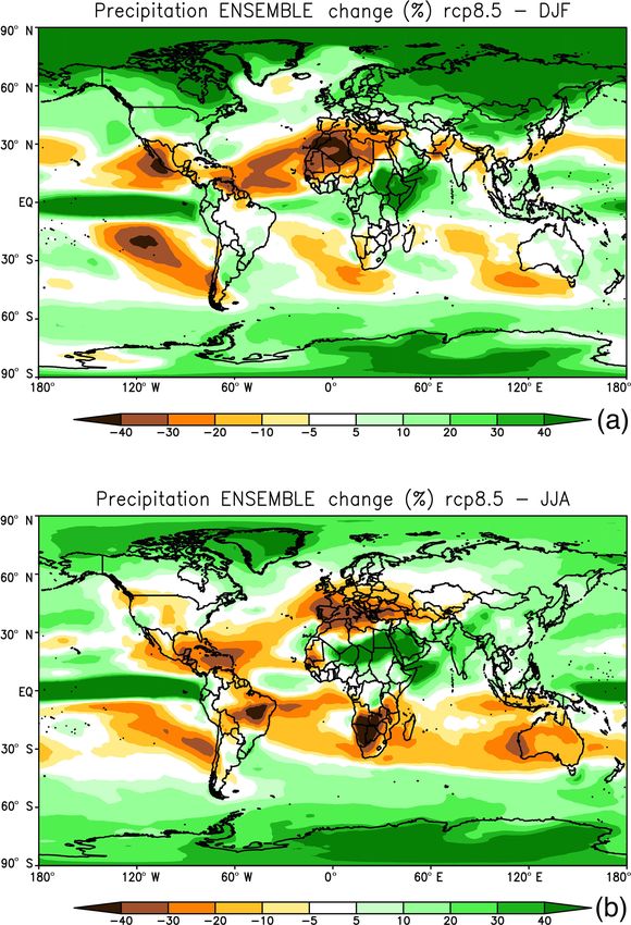
74                                                F. Giorgi et al.: Response of precipitation characteristics to global warming

ture only from an area about 3–5 times the size of the event          In the next sections we first summarize the changes in
itself (Trenberth et al., 2003). In addition, on average, only     mean precipitation fields in our ensemble of model projec-
about 25 % of days are rainy days, but since it does not rain      tions and then explore the response of different precipita-
throughout the entire day, the actual fraction of time it rains    tion characteristics, trying specifically to identify robust re-
has been estimated at 5 %–10 % (Trenberth et al., 2003). In        sponses. After having identified the dominant hydroclimatic
other words, most of the time it does not actually rain.           responses, we discuss examples of their impact on different
   This has important implications for the assessment of hy-       quantities of relevance for socioeconomic impacts, specifi-
droclimatic responses to global warming because it may not         cally the potential stress associated with changes in dry and
be very meaningful, and certainly not sufficient, to analyze       wet extreme events, precipitation interannual variability, and
mean precipitation fields, but it is necessary to also investi-    the predictability of precipitation events.
gate higher-order statistics. For example, the same mean of
1 mm day−1 could derive from 10 consecutive 1 mm day−1             2     The hydroclimatic response to global warming
events, a single 10 mm day−1 event with 9 dry days or two
5 mm day−1 events separated by a dry period. Each of these         Throughout this paper we mostly base our analysis on the
cases would have a very different impact on societal sectors       10 CMIP5 GCMs used by Giorgi et al. (2014a) for eas-
or ecosystem dynamics.                                             ier comparison with, and reference to, this previous work.
   This consideration also implies that the impact of global       These 10 models were chosen because they were the only
warming on the Earth’s hydroclimate might actually mani-           ones among the full CMIP5 dataset for which daily data were
fest itself not only as a change in mean precipitation but also,   available at the time the analysis of Giorgi et al. (2014a) was
perhaps more markedly, as variations in the characteristics        carried out. This sub-ensemble includes some of the most
and regimes of precipitation events. This notion has been in-      commonly used models, and an analysis of mean and sea-
creasingly recognized since the pioneering works of Tren-          sonal data by Giorgi et al. (2014a) showed that it behaves
berth (1999) and Trenberth et al. (2003), with many studies        quite similarly to the full CMIP5 ensemble. In addition, as
looking particularly at changes in the frequency and intensity     will be seen later, a high level of consistency is found in the
of extreme precipitation events (e.g., Easterling et al., 2000;    behavior of these models also concerning daily statistics, and
Christensen and Christensen, 2003; Tebaldi et al., 2006; Al-       therefore we feel that this 10-GCM ensemble is at least qual-
lan and Soden, 2008; Giorgi et al., 2011, 2014a, b; IPCC,          itatively representative of the full CMIP5 set.
2012; Sillmann et al., 2013b; Pendergrass and Hartmann,
2014; Sedlacek and Knutti, 2014; Pfahl et al., 2017; Thack-
                                                                   2.1    Mean precipitation changes
eray et al., 2018).
   In this paper, which presents a synthesis of the Alexander      In general, as a result of the warming of the oceans and land,
von Humboldt medal lecture given by the first author (FG) at       global surface evaporation increases with increasing GHG
the European Geosciences Union (EGU) General Assembly              forcing. This increase mostly lies in the range of 1 %–2 % per
in 2018, we revisit some of the concepts related to the issue      degree of surface global warming (% per DGW; Trenberth et
of the impacts of global warming on the characteristics of         al., 2007). As a consequence, global mean precipitation also
the Earth’s hydroclimate, stressing that it is not our purpose     tends to increase roughly by the same amount. This has been
to provide a review of the extensive literature on this topic.     found in most GCM projections, as illustrated in the exam-
Rather, we want to illustrate some of the points made above        ples in Fig. 1.
through relevant examples obtained from new and past anal-            Although precipitation increases globally, at the regional
yses of global and regional climate model projections carried      level we can find relatively complex patterns of change, with
out by the authors.                                                areas of increased and areas of decreased precipitation. These
   More specifically, we will draw from global climate model       patterns are closely related to changes in global circulation
(GCM) projections carried out as part of the CMIP5 program         features, global energy and momentum budgets, local forc-
(Taylor et al., 2012) and regional climate model (RCM) pro-        ings (e.g., topography, land use), and energy and water fluxes
jections from the COordinated Regional climate Downscal-           affecting convective activity (e.g., Thackeray et al., 2018).
ing EXperiment (CORDEX; Giorgi et al., 2009; Jones et al.,         The basic geographical structure of precipitation change pat-
2011; Gutowski Jr. et al., 2016), which downscale CMIP5            terns has been quite resilient throughout different generations
GCM data. In this regard, we focus on the high-end RCP8.5          of GCM projections, at least in an ensemble-averaged sense.
scenario (Moss et al., 2010), in which the ensemble mean           These precipitation change patterns are shown in Fig. 2 as
global temperature increase by 2100 is about 4 ◦ C (±1 ◦ C)        obtained from the CMIP5 ensemble, but they are similar in
compared to late 20th century temperatures (IPCC, 2013),           the CMIP3 and earlier GCM ensembles.
stressing that results for lower GHG scenarios are qualita-           The increase in precipitation at middle to high latitudes has
tively similar to those found here but of smaller magnitude        been attributed to a poleward shift of the storm tracks associ-
(not shown for brevity).                                           ated with maximum warming in the tropical troposphere (due
                                                                   to enhanced convection), which in turn produces a poleward

Earth Syst. Dynam., 10, 73–89, 2019                                                    www.earth-syst-dynam.net/10/73/2019/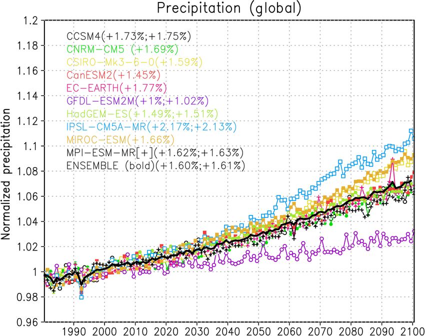
F. Giorgi et al.: Response of precipitation characteristics to global warming                                                          75

Figure 1. Normalized mean global precipitation from 1981 to 2100
in the 10 CMIP5 GCM simulations for the RCP8.5 scenario used
by Giorgi et al. (2014a), along with their ensemble average. The
first number in parentheses shows the corresponding mean global
precipitation change per degree of global warming, while the sec-
ond shows (for a subset of models with available data) the same
quantity for global surface evaporation. The annual precipitation is
normalized by the mean precipitation during the reference period
1981–2010; therefore, a value of, e.g., 1.1 indicates an increase of
10 %.

shift of the maximum horizontal temperature gradient and jet
stream location (e.g., IPCC, 2013). This process is essentially
equivalent to a poleward expansion of the Hadley cell, which           Figure 2. Ensemble mean change in precipitation (RCP8.5, 2071–
also causes drier conditions in subtropical areas, including           2100 minus 1981–2010) for December–January–February (a) and
the Mediterranean and Central America–Southwestern US                  June–July–August (b) in the CMIP5 ensemble of models.
regions. The Intertropical Convergence Zone (ITCZ) shows
narrowing and greater precipitation intensity, especially in
the core of the Pacific ITCZ, associated with increased orga-          wards the upwind side of the mountains and to reduce the
nized deep convective activity towards the ITCZ center and             increases or even generate decreases in precipitation in the
decreased activity along its edges (Byrne et al., 2018). Fi-           lee side (e.g., Giorgi et al., 1994; Gao et al., 2006). Sim-
nally, over monsoon regions, a general increase in precipi-            ilarly, in the summer, the precipitation change signal can
tation has been attributed to a greater water-holding capac-           be strongly affected by high-elevation warming and wet-
ity of the atmosphere counterbalancing a decrease in mon-              ting, which enhance local convective activity. For example,
soon circulation strength (IPCC, 2013); however, more de-              Giorgi et al. (2016) found enhanced precipitation over the
tailed analyses of how global constraints on energy and mo-            Alpine high peaks in high-resolution EURO-CORDEX (Ja-
mentum budgets affect regional-scale circulations are needed           cob et al., 2014) and MED-CORDEX (Ruti et al., 2016) pro-
for a better understanding of the monsoon response to global           jections, whereas the driving coarse-resolution global mod-
warming (Biasutti et al., 2018).                                       els produced a decrease in precipitation. In addition to these
   As already mentioned, these broad-scale change patterns             local effects, it has been found that the simulation of some
have been confirmed by different generations of GCM pro-               modes of variability, such as blocking events, is also sensi-
jections and thus appear to be robust model-derived signals.           tive to model resolution (e.g., Anstey et al., 2013; Schiemann
On the other hand, high-resolution RCM experiments have                et al., 2017). As a result of all these processes it is thus possi-
shown that local forcings associated with complex topogra-             ble that the large-scale precipitation change patterns in Fig. 2
phy and coastlines can substantially modulate these large-             might be significantly modified as we move to substantially
scale signals, often to the point of being of opposite sign. For       higher-resolution models.
example, the precipitation shadowing effect of major moun-                On the other hand, a key question concerning the precipi-
tain systems tends to concentrate precipitation increases to-          tation response to global warming is the following: How will

www.earth-syst-dynam.net/10/73/2019/                                                          Earth Syst. Dynam., 10, 73–89, 2019
76 F. Giorgi et al.: Response of precipitation characteristics to global warming
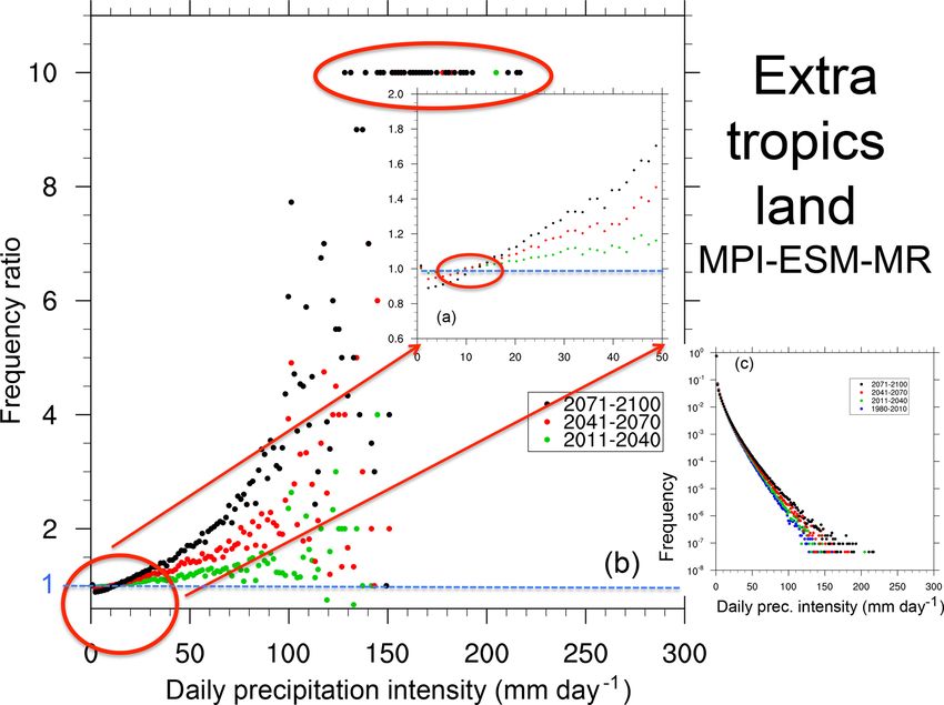
precipitation change patterns affect different socioeconomic Figs. 3 and 4 report the ratio of the frequency of occurrence
sectors? This question depends more on the modifications of for a given bin in a future time slice divided by the same
the characteristics of precipitation than the mean precipita- quantity in the reference period. Averaged data are shown
tion itself. For example, changes in precipitation interannual for land areas in the tropics (30◦ S–30◦ N; Fig. 3) and extra-
variability may have strong impacts on crop planning. As an- tropical midlatitudes (30–60◦ N and S; Fig. 4), noting that
other example, if an increase in precipitation is due to an in- qualitatively similar results were found for ocean areas.
crease in extreme damaging events, this will have negative The PDFs exhibit a log-linear relationship between inten-
rather than positive impacts. Alternatively, if the increase is sities and frequencies, with a sharp drop in frequency as the
due to very light events that do not replenish the soil of mois- intensity increases. The ratios of future vs. present-day fre-
ture, this will not constitute an added water resource. Con- quencies consistently show the following features.
versely, a reduction of precipitation mostly associated with a
reduction of extremes will result in positive rather than neg- 1. An increase in the number of dry days, as seen from
ative impacts. It is thus critical to assess how the character- the ratios > 1 in the first bin (precipitation less than
istics of precipitation will respond to global warming, which 1 mm day−1 ), i.e., a decrease in the frequency of wet
is the focus of the next sections. events. Note that, even if these ratios are only slightly
greater than 1, because the frequencies of dry days are
much higher than those of wet days, the actual absolute
2.2 Daily precipitation intensity probability density increase in the number of dry days is relatively high.
functions (PDFs)
2. A decrease (ratio < 1) in the frequency of light to
Daily precipitation is one of the variables most often used
medium precipitation events up to a certain intensity
in impact assessment studies, and therefore an effective way
threshold. In the models we analyzed, when taken over
to investigate the response of precipitation characteristics to
large areas, this threshold lies around the 95th percentile
global warming is to assess changes in daily precipitation
of the full distribution and is higher for tropical than ex-
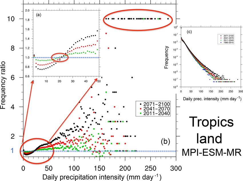
intensity PDFs. As an illustrative example of PDF changes,
tratropical land regions because of the higher amounts
Figs. 3 and 4 show normalized precipitation intensity PDFs
of precipitation in tropical convection systems. Inter-
for four time slices: 1981–2010 (reference period representa-
estingly, while the threshold depends on latitude, it is
tive of present-day conditions), 2011–2040, 2041–2070 and
approximately invariant for all future time slices, i.e.,
2071–2100 in the MPI-ESM-MR RCP8.5 projection of the
it appears to be relatively independent of the level of
CMIP5 ensemble. The further the time slice is in the future,
warming. The decrease in light precipitation events has
the greater the warming (up to a maximum of about 4 ◦ C in
been at least partially attributed to an increase in ther-
2071–2100). The variable shown, which we refer to as PDF,
mal stability induced by the GHG forcing (Chou et al.,
is the frequency of occurrence of precipitation events within
2012).
a certain interval (bin) of intensity normalized by the total
number of days, including non-precipitating days. 3. An increase (ratio > 1) in the frequency of events for
Note that in the MPI-ESM-MR model the response of intensities higher than the threshold mentioned above.
mean global precipitation to global warming is in line with The relative increase in frequency grows with the in-
the model ensemble average (Fig. 1), while the response of tensity of the events, and it is thus maximum for the
daily statistics is among the strongest (see, e.g., Giorgi et al., highest-intensity events, an indication of a nonlinear re-
2014a and Table 1), but qualitatively consistent with most sponse of the precipitation intensity to warmer condi-
other models (see below). Therefore, this model is illustrative tions. Note that, because of the logarithmic frequency
of the simulated precipitation response to global warming in scale, the absolute increase in the number of high-
the subset of CMIP5 GCMs analyzed. intensity events is relatively low.
Also, as in our previous work (Giorgi et al., 2014a),
throughout this paper a rainy day is considered as having 4. The occurrence in future time slices of events with inten-
a precipitation amount of at least 1 mm day−1 so that driz- sity well beyond the maximum found in the reference pe-
zle days are removed. In this regard, the choice of a pre- riod. These are illustrated by the prescribed value of 10
cipitation threshold to define a rainy day makes the calcu- when events occurred for a given bin in the future time
lation of precipitation frequency and intensity dependent on slice, but not in the reference one. One could thus inter-
the resolution of the data (e.g., Chen and Dai, 2018). Atten- pret these as occurrences of “unprecedented” events.
tion should be paid to this issue when analyzing precipitation
statistics and here, as well as in previous work, we conduct 5. All the features 1–4 tend to amplify as the time slice is
direct cross-model or data–model intercomparisons only af- further into the future, i.e., as the level of warming in-
ter having interpolated the data onto common grids. creases, and are generally more pronounced over trop-
Finally, given the logarithmic scale of the frequency of oc- ical than extratropical areas (and over land than ocean
currence, in order to better illustrate changes in frequencies, regions, which we did not show for brevity).
Earth Syst. Dynam., 10, 73–89, 2019 www.earth-syst-dynam.net/10/73/2019/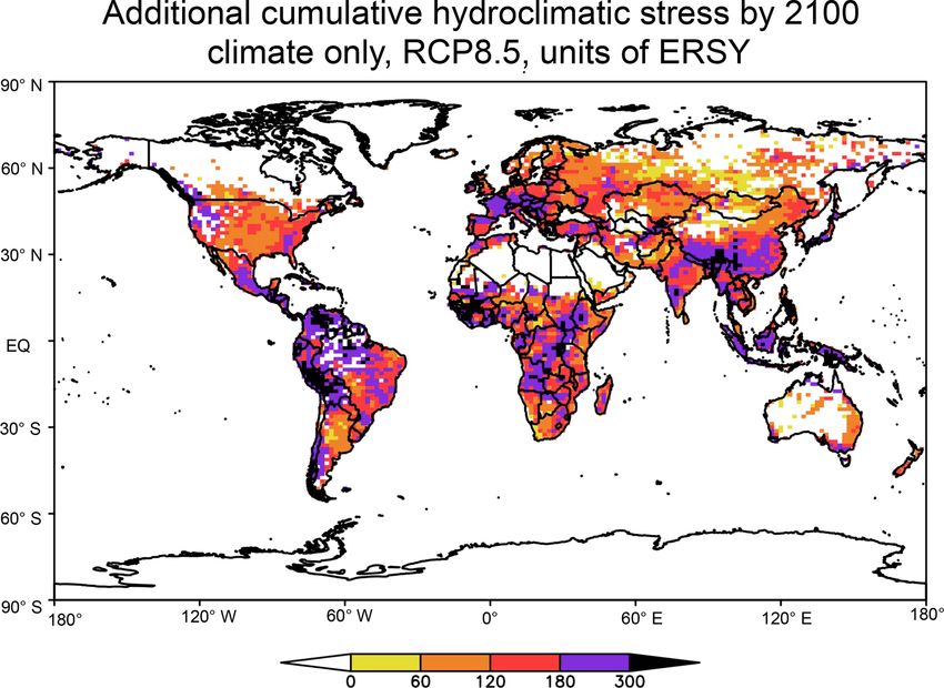
F. Giorgi et al.: Response of precipitation characteristics to global warming                                                          77

Table 1. Change in different daily precipitation indicators between 2071–2100 and 1976–2005 for the 10 CMIP5 GCMs of Giorgi et
al. (2014a) expressed in % per degree of surface global warming over global (upper box) and global land (lower box) areas; “global”
means the area between 60◦ S and 60◦ N. SDII is the precipitation intensity, 95p, 99p and 99.9p are the 95th, 99th and 99.9th percentiles,
respectively, and the precipitation change only include wet days, i.e., days with precipitation greater than 1 mm day−1 .

  Models              No. wet days     Precipitation change (due to    SDII change       95p change       99p change      99.9p change
                      % per DGW             wet days) % per DGW       (%) per DGW      (%) per DGW      (%) per DGW      (%) per DGW
  Global box
  HadGEM-ES                   −0.7                             1.3              1.8               1.7              2.9              3.9
  MPI-ESM-MR                  −2.4                             1.0              3.5               1.9              3.7              5.3
  GFDL-ESM2M                  −1.4                            0.05              1.2               0.3              2.1             10.4
  IPSL-CM5A-MR                −1.0                             1.6              2.6               2.0              4.5              7.9
  CCSM4                       −1.1                             0.7              1.8               1.1              2.8              5.5
  CanESM2                     −0.4                             1.6              1.7               1.5              2.5              4.4
  EC-EARTH                    −0.9                             1.3              2.1               1.9              3.7              5.9
  MIROC-ESM                    0.2                             1.4              0.9               1.1              1.2              1.6
  CSIRO-Mk3-6-0               −0.6                             0.8              1.9               2.3              2.4              3.4
  CNRM-CM5                    −0.1                             1.4              1.5               1.5              2.9              5.8
  Ensemble                    −0.8                             1.1              1.9               1.5              2.9              5.4
  Global land box
  HadGEM-ES                   −1.4                            0.7               2.1               1.2              2.8              4.5
  MPI-ESM-MR                  −3.3                            0.1               4.0               0.8              3.7              5.4
  GFDL-ESM2M                  −1.8                            1.1               3.1               1.2              4.5             12.4
  IPSL-CM5A-MR                −1.8                            0.7               2.5               1.2              3.8              7.2
  CCSM4                       −0.6                            1.3               1.9               1.3              2.8              5.4
  CanESM2                     −0.6                            1.2               1.7               1.3              3.4              5.0
  EC-EARTH                    −0.8                            1.4               2.3               2.0              3.8              6.0
  MIROC-ESM                    0.2                            1.8               1.4               1.1              1.7              2.1
  CSIRO-Mk3-6-0               −1.8                           −0.2               1.5               0.2              1.1              2.4
  CNRM-CM5                     0.4                            2.5               2.0               2.0              3.2              6.0
  Ensemble                    −1.2                             1.1              2.3               1.2              3.1              5.6

Although the results in Figs. 3 and 4 are obtained from one            RCM projections (e.g., Gutowski Jr. et al., 2007; Boberg et
model, they are qualitatively consistent with those we found           al., 2009; Jacob et al., 2014; Giorgi et al., 2014b), suggesting
for other CMIP5 GCMs. As an example, results analogous                 that the projected changes in the precipitation intensity PDFs
to those in Figs. 3 and 4, but for the HadGEM and EC-Earth             summarized in points 1–4 above are generally robust across
GCMs, are reported in Supplement Figs. S1 and S2. We also              a wide range of models and model resolutions.
carried out the same type of analysis for a high-resolution
RCM projection (12 km grid spacing, RCP8.5 scenario) con-
ducted with the RegCM4 model (Giorgi et al., 2012) over                2.3   Hydroclimatic indices
the Mediterranean domain defined for the MED-CORDEX                    The changes in precipitation intensity PDFs found in the
program (Ruti et al., 2016). Figures 5 and 6 show PDFs                 previous section should be reflected in, and measured by,
and PDF ratios for three 30-year future time slices calcu-             changes in hydroclimatic indices representative of given pre-
lated over land areas throughout the Mediterranean domain              cipitation regimes. In two previous studies (Giorgi et al.,
and over a subarea covering the Alpine region. They show               2011, 2014a), we assessed the changes in a series of intercon-
features similar to those found for the GCMs, with the sig-            nected hydroclimatic indices in an ensemble of 10 CMIP5
nal over the Alpine region being more pronounced than for              projections. The indices analyzed include the following.
the entire Mediterranean area. As further examples, Supple-
ment Figs. S3 and S4 report similar plots computed over the               – SDII: mean precipitation intensity (including only wet
entire European land territory for EURO-CORDEX simula-                      events)
tions with the REMO and RACMO RCMs, which show fea-
tures qualitatively in line with those of Figs. 5 and 6. In addi-         – DSL: mean dry spell length, i.e., mean length of con-
tion, our results are also consistent with previous analyses of             secutive dry days

www.earth-syst-dynam.net/10/73/2019/                                                           Earth Syst. Dynam., 10, 73–89, 2019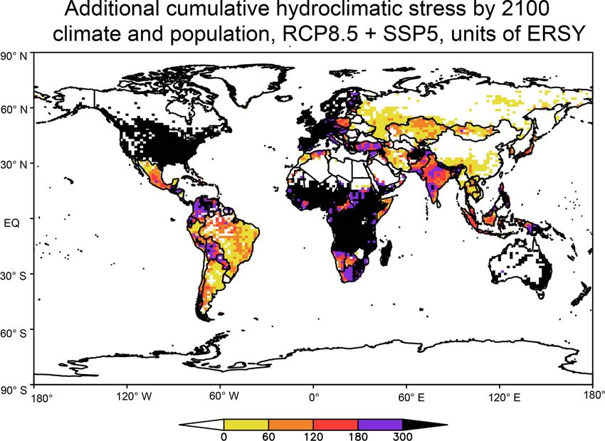
78                                                    F. Giorgi et al.: Response of precipitation characteristics to global warming

Figure 3. (a) A zoomed-in view of the part of the curves highlighted by the corresponding red oval. Ratio values of 10 (highlighted with a
red oval) are used when events occur in the future time slice that are not present in the reference period for a given intensity bin. (b) Ratio
of future to reference normalized frequency of daily precipitation intensity for the three future time slices. (c) Probability density function
(PDF) defined as the normalized frequency of occurrence of daily precipitation events of intensity within a certain bin interval over land
regions in the tropics (30◦ S–30◦ N) for the reference period 1981–2010 and three future time slices (2011–2040, 2041–2070, 2071–2100) in
the MPI-ESM-MR model. The frequency is normalized by the total number of days (including dry days, i.e., days with precipitation lower
than 1 mm day−1 ).

  – WSL: mean wet spell length, i.e., mean length of con-                 as well as a number of RCM projections, in future time slices
    secutive wet days                                                     with respect to the 1976–2005 reference period. Their re-
                                                                          sults, which were consistently found for most models ana-
  – R95: fraction of total precipitation above the 95th per-              lyzed, indicated a prevalent increase in SDII, R95, HY-INT
    centile of the daily precipitation intensity distribution             and DSL and a decrease in PA and WSL. Similar results were
    during the reference period 1981–2010                                 then found by Giorgi et al. (2014b) in an analysis of multiple
                                                                          RegCM4-based projections over five CORDEX domains. In
  – PA: precipitation area, i.e., the total area covered by wet
                                                                          other words, under warmer climate conditions, precipitation
    events on any given day
                                                                          events are expected to be more intense and extreme and are
  – HY-INT, i.e., the hydroclimatic intensity index intro-                temporally more concentrated and less frequent, which im-
    duced by Giorgi et al. (2011) consisting of the product               plies a reduction of the areas occupied by rain at any given
    of normalized SDII and DSL                                            time (although not necessarily a reduction of the size of the
                                                                          events). This response, which is consistent with the change in
Note that the PA and HY-INT indices were specifically in-                 PDFs illustrated in Figs. 3–6, will hereafter be referred to as
troduced by Giorgi et al. (2011, 2014a). The PA is the spa-               the higher intensity-reduced frequency (HIRF) precipitation
tial counterpart of the mean frequency of precipitation days,             response.
while the HY-INT was introduced under the assumption that                    Giorgi et al. (2011, 2014a) also analyzed a global and sev-
the changes in SDII and DSL are interconnected responses                  eral regional daily precipitation gridded observation datasets
to global warming (Giorgi et al., 2011).                                  and found that trends for the period 1976–2005 were pre-
   Giorgi et al. (2011, 2014a) examined changes in these in-              dominantly in line with the model-projected changes over
dices for ensembles of CMIP3 and CMIP5 GCM projections,

Earth Syst. Dynam., 10, 73–89, 2019                                                             www.earth-syst-dynam.net/10/73/2019/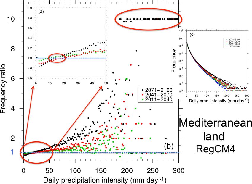
F. Giorgi et al.: Response of precipitation characteristics to global warming                                                   79

Figure 4. Same as Fig. 3 but for extratropical land areas.

most continental areas. Further evidence of increases in            mean precipitation, which implies a decrease in precipitation
heavy precipitation events in observational records is, for ex-     frequency.
ample, reported by Fischer and Knutti (2016) and references            To illustrate this point, Table 1 reports the globally aver-
therein; however, this conclusion cannot be considered en-          aged changes (2071–2100 minus the reference period 1976–
tirely robust and needs to be verified with further analysis        2005, as in Giorgi et al., 2014a; RCP8.5 scenario) in mean
due to the high uncertainty in precipitation observations (e.g.,    precipitation, precipitation intensity and frequency, and the
Herold et al., 2017).                                               95th, 99th and 99.9th percentiles of daily precipitation for
   An explanation for the HIRF hydroclimatic response to            the 10 GCMs of Giorgi et al. (2014a), along with their
global warming is related to the fact that, on the one hand,        ensemble average. The values of Table 1 were calculated
the mean global precipitation change roughly follows the            as follows: we first computed the change in % per DGW
mean global evaporation increase, i.e., 1.5–2.0 % per DGW           at each model grid point and then averaged these values
(Trenberth et al., 2007, Fig. 1). On the other hand, the in-        over global land + ocean as well as global land-only areas.
tensity of precipitation, in particular for high and extreme        This was done in order to avoid the possibility that areas
precipitation events, is more tied to the increase in the water-    with large precipitation amounts may dominate the average.
holding capacity of the atmosphere, which is in turn regu-          On the other hand, grid-point normalization artificially am-
lated by the Clausius–Clapeyron (Cl–Cl) response of about           plifies the contribution of regions with small precipitation
7 % per DGW, although the precipitation response is mod-            amounts, such as polar and desert areas. For this reason, as
ulated by regional and local circulations along with energy         in Giorgi et al. (2014a), we did not include in the averag-
and water fluxes, which might lead to super-Cl–Cl or sub-           ing areas north of 60◦ N and south of 60◦ S (polar regions)
Cl–Cl responses (e.g., Trenberth et al., 2003; Pall et al., 2007;   along with areas with mean annual precipitation lower than
Lenderink and van Meijgaard, 2008; Chou et al., 2012; Sin-          0.5 mm day−1 (which effectively identifies desert regions). In
gleton and Toumi, 2013; Pendergrass and Hartmann, 2014;             addition, we did not consider precipitation associated with
Ivancic and Shaw, 2016; Fischer and Knutti, 2016; Pfahl et          days with amounts of less than 1 mm day−1 in order to be
al., 2017). Therefore, the increase in precipitation intensity      consistent with our definition of a rainy day (which disre-
can be expected to be generally larger than the increase in         gards drizzle events).

www.earth-syst-dynam.net/10/73/2019/                                                      Earth Syst. Dynam., 10, 73–89, 2019
80                                                F. Giorgi et al.: Response of precipitation characteristics to global warming

Figure 5. Same as Fig. 3 but for Mediterranean land areas in a MED-CORDEX experiment with the RegCM4 RCM driven by global fields
from the HadGEM GCM.

   Also in these calculations, the increase in global mean pre-    to the fact that precipitation intensity, especially for intense
cipitation is in the range of 1% per DGW to 2 % per DGW            events (beyond the 95th percentile), responds at the local
except for the GFDL experiment, which shows a very small           level primarily to the Cl–Cl-driven increase in water vapor
increase (indicating that in this model most of the precipi-       amounts modulated by local circulations and fluxes, while
tation increase occurs in the polar regions). In all cases ex-     mean precipitation responds to a slower evaporation process,
cept for MIROC the increase in global SDII is greater than         driving a decrease in precipitation frequency. Noticeably, the
the increase in mean precipitation, resulting in a decrease        MIROC experiment does not appear to follow this response;
in the number of rainy days. The changes in the 95th, 99th         i.e., in this model the increase in mean precipitation appears
and 99.9th percentiles are maximum for the most extreme            to be driven by an increase in the number of light precipita-
percentiles, showing that the main contribution to the HIRF        tion events.
response is due to the highest-intensity events, i.e., above          While the data in Table 1 provide a diagnostic explanation
the 99th and 99.9th percentiles, whose response becomes in-        for the HIRF response, it has also been suggested by very-
creasingly closer to the Cl–Cl one (and even super-Cl–Cl for       high-resolution convection-permitting simulations that ocean
the GFDL model). In fact, the increase in the 95th percentile      temperatures might affect the self-organization and aggrega-
for the ensemble model average is lower than the increase in       tion of convective systems (e.g., Mueller and Held, 2012;
SDII, and this is because in some models the threshold inten-      Becker et al., 2017), which would also affect the precipita-
sity in Figs. 3–6, for which the sign of the change turns from     tion response to warming. Therefore, the study of the HIRF
negative to positive, lies beyond the 95th percentile. When        response might lead to a greater understanding of the funda-
only land areas between 60◦ S and 60◦ N are taken into ac-         mental behavior of the precipitation phenomenon, in partic-
count (bottom panel in Table 1), the changes are generally in      ular tropical convection processes.
line with the global ones, except for the CNRM model. Over
land areas we also find changes in the highest percentiles of      3   Some consequences of the hydroclimatic
magnitude mostly greater than over the globe (and thus over            response to global warming
oceans).
   We can thus conclude that the shift to a regime of more         What are the consequences of the HIRF response to global
intense but less frequent events in warmer conditions is due       warming? Obviously there can be many of them, but here we

Earth Syst. Dynam., 10, 73–89, 2019                                                    www.earth-syst-dynam.net/10/73/2019/
F. Giorgi et al.: Response of precipitation characteristics to global warming                                                  81

Figure 6. Same as Fig. 5 but for the Alpine region.

want to provide a few illustrative examples of relevance for       sociated with these extremes is proportional to the excess
impact applications.                                               precipitation above the 99.9th percentile of the distribution.
                                                                   GCR18 calculated this quantity for a future climate projec-
                                                                   tion and then normalized it by the corresponding value cumu-
3.1   Potential stress associated with wet and dry                 lated over the reference period. This normalization expresses
      extreme events                                               the potential stress due to the increase in wet extremes
                                                                   in equivalent reference stress years (ERSYs), whereby an
The HIRF response suggests that global warming might in-
                                                                   ERSY is the mean stress per year due to the extremes during
duce an increase in the risk of damaging extreme wet and dry
                                                                   the reference period (in our case 1981–2010). If, for example,
events, the former being associated with the increase in pre-
                                                                   a damage value can be assigned to such events, the ERSY
cipitation intensity and latter with the occurrence of longer
                                                                   can be interpreted as the mean yearly damage caused by ex-
sequences of dry days over areas of increasing size. In order
                                                                   tremes in present climate conditions. GCR18 then carried out
to quantify this risk, in a recent paper (Giorgi et al., 2018;
                                                                   similar calculations for the cumulative potential stress due to
hereafter referred to as GCR18) we introduced a new index
                                                                   dry events by cumulating the deficit rain defined by the D25
called the Cumulative Hydroclimatic Stress Index, or CHS.
                                                                   metric. In addition, similarly to Diffenbaugh et al. (2007) and
In GCR18, the CHS was calculated for two types of extreme
                                                                   Sedlacek and Knutti (2014), they included exposure informa-
events, the 99.9th percentile of the daily precipitation distri-
                                                                   tion within the definition of the CHS index by multiplying the
bution (or R99.9) and the occurrence of at least three con-
                                                                   excess or deficit precipitation by future population amounts
secutive months experiencing a precipitation deficit with a
                                                                   (as obtained from Shared Socioeconomic Pathways, or SSPs;
magnitude greater than 25 % of the precipitation climatology
                                                                   Rihai et al., 2016) normalized by present-day population val-
for that month (or D25). Both of these metrics thus refer to
                                                                   ues. The details of these calculations can be found in GCR18.
extremely wet and dry events that can be expected to produce
                                                                      The main results of GCR18 are summarized in Figs. 7 and
significant damage (see GCR18).
                                                                   8, which present maps of the potential cumulative stress due
   Taking as an example the R99.9, the CHS essentially cu-
                                                                   to both dry and wet events added by climate change dur-
mulates the excess precipitation above the 99.9th percentile
                                                                   ing the period 2010–2100 and expressed in added ERSYs
threshold calculated for a given reference period (e.g., 1981–
                                                                   (i.e., after removing the value of 90 that would be obtained
2010). Hence, the assumption is that the potential stress as-

www.earth-syst-dynam.net/10/73/2019/                                                     Earth Syst. Dynam., 10, 73–89, 2019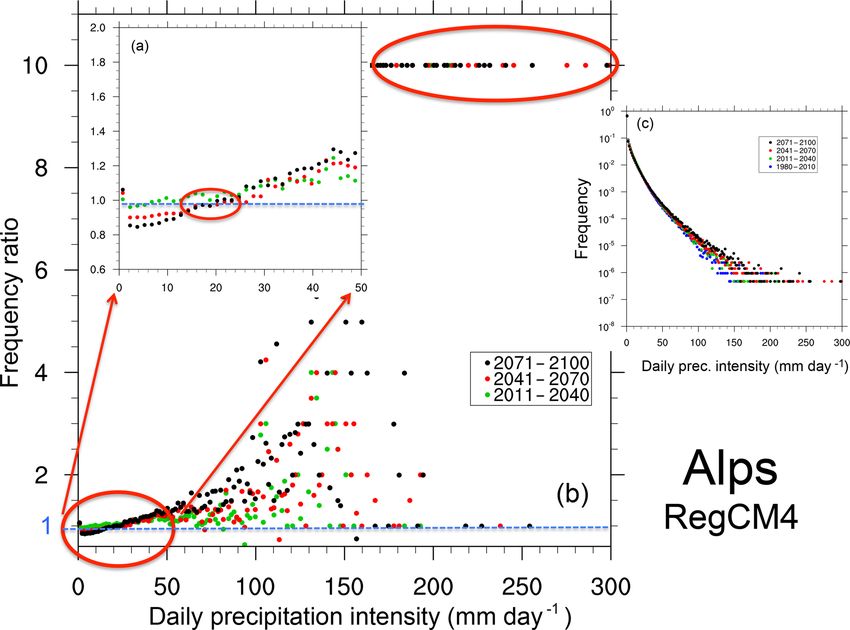
82                                                F. Giorgi et al.: Response of precipitation characteristics to global warming

if no climate change occurred). The figures show the total         though some works suggest the presence of robust changes in
ensemble-averaged added cumulative stress for the RCP8.5           projected spatial patterns of ENSO-driven precipitation and
scenario without (Fig. 7) and with (Fig. 8) the inclusion of       temperature variability (e.g., Power et al., 2013).
population weighting (for which the SSP5 population sce-              Daily and seasonal precipitation statistics are not neces-
nario from Rihai et al., 2016, was used). The values in the        sarily tied, since the same seasonal mean can be obtained via
figures were computed by first calculating the stress contri-      different sequences of daily precipitation events. In addition,
bution in ERSYs of wet and dry extremes separately and then        the intensity distribution of daily and seasonal precipitation
adding them so that there is no cancellation of stress if, for     amounts can be quite different, the latter often being close to
example, a wet extreme is followed by a dry extreme.               normal distributions (e.g., Giorgi and Coppola, 2009). On the
   Figure 7 shows that, when only climate is accounted for,        other hand, the occurrence of longer dry spells, intensified by
dry and wet extremes add more than 180 ERSYs (and in               higher temperatures and lower soil moisture amounts, might
some cases more than 300 ERSYs) over extended areas of             be expected to amplify dry seasons, while the increase in the
Central and South America, Europe, western and south–              intensity of sequences of wet events might lead to amplified
central Africa, and southern and southeastern Asia. In other       wet seasons. As a result, it can be expected that the HIRF
words, the combined potential stress due to dry and wet ex-        regime response might lead to an increase in precipitation
tremes more than triples due to climate change by the end of       interannual variability.
the century. In this regard, GCR18 found that, when globally          To verify this hypothesis, we calculated for the GCM en-
averaged over land regions and over all the models consid-         semble of Giorgi et al. (2014a) the change in precipitation in-
ered, both wet and dry extremes increased in the RCP8.5 sce-       terannual variability between future and present-day 30-year
nario, the former adding ∼ 120 ERSYs and the latter adding         time slices using as a metric the coefficient of variation (CV).
∼ 30 ERSYs.                                                        The CV is defined as the (in our case interannual) standard
   When population scenarios are also accounted for (Fig. 8)       deviation normalized by the mean and has often been used as
the patterns of added cumulative stress are considerably           a measure of precipitation variability because it removes the
modified. In this case, the total number of added ERSYs ex-        strong dependence of precipitation variability on the mean
ceeds 300 over the entire continental US and Canada, most          itself (Raisanen, 2002; Giorgi and Bi, 2005).
of Africa, Australia, and areas of South and Southeast Asia,          Figure 9 shows the ensemble average change in precipita-
which are projected to experience substantial population in-       tion CV between the 2071–2100 and 1981–2010 time slices
creases in the SSP5 scenario. Conversely, we find a reduced        for mean annual precipitation as well as precipitation av-
increase in stress over East and Southeast Asia, where the         eraged over the two 6-month periods April–September and
population is actually projected to decrease by the end of         October–March. It can be seen that, when considering an-
the 21st century (see GCR18). This result thus points to the       nual averages, the interannual variability increases over the
importance of incorporating socioeconomic information in           majority of land areas, with exceptions over small regions
the assessment of the stress associated with climate-change-       scattered throughout the different continents. When consid-
driven extreme events.                                             ering the two different 6-month seasons, in April–September
   Notwithstanding the limitations and approximations of the       (Northern Hemisphere summer, Southern Hemisphere win-
approach of GCR18 amply discussed in that paper, the results       ter) variability increases largely dominate, except over areas
in Figs. 7 and 8 clearly indicate that the increase in wet and     of the Northern Hemisphere high latitudes and some areas
dry extremes associated with global warming can constitute         around major mountain systems. In October–March, the ar-
a serious threat to the socioeconomic development of vari-         eas of decreased variability are more extended over north-
ous regions across all continents. GCR18 also show that the        ern Eurasia, northern North America and, interestingly, some
cumulative stress due to increases in extremes is drastically      equatorial African regions, although the increases are still
reduced under the RCP2.6 scenario, pointing to the impor-          somewhat more widespread.
tance of mitigation measures to reduce the level of global            Although Fig. 9 does not show a signal of ubiquitous sign
warming.                                                           across all land areas, it clearly points to a prevalent increase
                                                                   in interannual variability associated with global warming,
3.2   Impact on interannual variability
                                                                   at least as measured by the CV. It is important to note that
                                                                   this increase occurs in areas of both increased and decreased
The interannual variability of precipitation is a key factor af-   mean precipitation (see Fig. 2), so it is not strongly related to
fecting many aspects of agriculture and water resources, and       the use of the CV as a metric. Finally, this result is broadly
it is strongly affected by global modes of variability, such       consistent with analyses of previous-generation model pro-
as the El Niño–Southern Oscillation (ENSO) in the tropics          jections (Raisanen, 2002; Giorgi and Bi, 2005; Pendergrass
and the North Atlantic Oscillation (NAO) in midlatitudes. In       et al., 2017), which adds robustness to this conclusion.
this regard, the latest generation of GCM projections does
not provide definitive indications concerning changes in the
frequency or intensity of such modes (e.g., IPCC, 2013), al-

Earth Syst. Dynam., 10, 73–89, 2019                                                    www.earth-syst-dynam.net/10/73/2019/
F. Giorgi et al.: Response of precipitation characteristics to global warming 83
Figure 7. Total number of additional stress years due to increases in wet (R99.9) and dry (D25) events for the period 2011–2100 including
only climate variables for the RCP8.5 scenario (see text for more detail). Units are equivalent reference stress years (ERSYs) and the value
does not include ERSYs obtained if climate did not change (i.e., for the period 2100–2011 a value of 90).
Figure 8. Same as Fig. 7, but with the inclusion of the SSP5 population scenario (see text for more detail).
3.3 Impact on precipitation predictability conomic activities (e.g., agriculture, hazards, tourism, etc.).
Indeed, precipitation is one of the most difficult meteorolog-
A third issue we want to address concerns the possible ef- ical variables to forecast, since it depends on both large-scale
fects of regime shifts on the predictability of precipitation, an and complex local-scale processes (e.g., topographic forc-
issue that has obvious implications for a number of socioe-
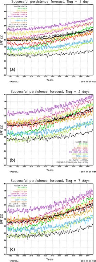
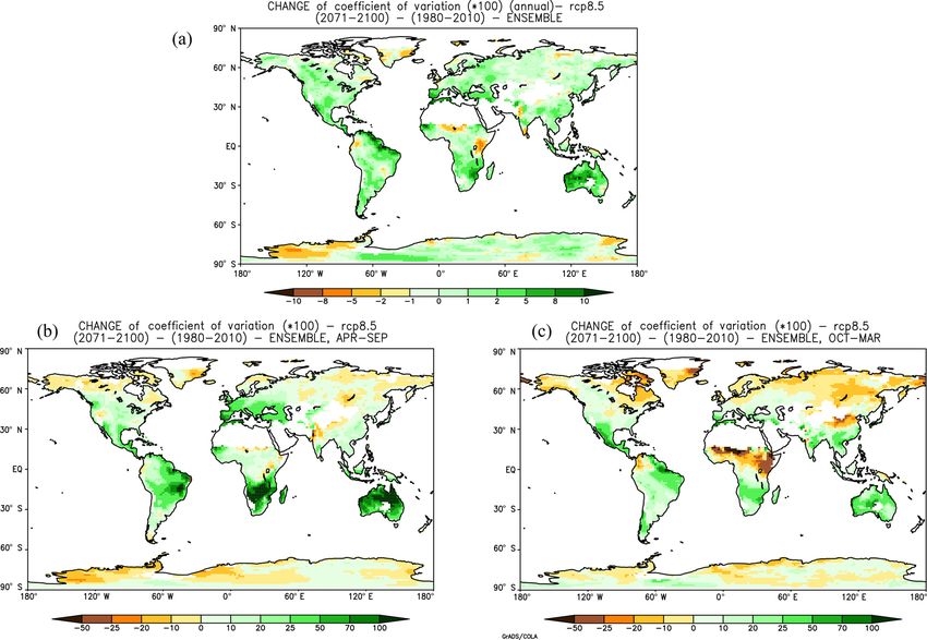
www.earth-syst-dynam.net/10/73/2019/ Earth Syst. Dynam., 10, 73–89, 201984 F. Giorgi et al.: Response of precipitation characteristics to global warming Figure 9. Change in precipitation interannual coefficient of variation (2071–2100 vs. 1981–2010) for (a) mean annual precipitation, (b) April–September precipitation and (c) October–March precipitation. ing). While the chaotic nature of the atmosphere provides a ing that the persistence forecast only concerns the occurrence theoretical limit to weather prediction of ∼ 10–15 days (e.g., of precipitation and not the amount. Warner, 2010), the predictability range of different types of Figure 10 shows that in all model projections, and thus in precipitation events depends crucially on the temporal scale the ensemble averages, the percent of successful persistence of the dynamics related to the event itself. For example, the forecasts increases with global warming for all three time predictability range of synoptic systems is of the order of lags. This can be mostly attributed to the increase in mean dry days, while that of long-lasting weather regimes, such as spell length found in Sect. 2. For a lag time of 1 day, the suc- blockings, can be of weeks. It is thus clear that changes in cessful persistence forecast in the model ensemble increases precipitation regimes and statistics can lead to changes in the globally from about 80 % in 2010 to about 83 % in 2100, potential predictability of precipitation. i.e., with a linear trend of ∼ 3.5 % per 100 years. As can be One of the benchmark metrics that is most often used to expected, the percentage of successful persistence forecasts assess the skill of a prediction system is persistence (Warner, decreases with the length of lag time: ∼ 76 % and 69 % in 2010). Essentially, persistence for a lead time T assumes that 2010 for lag times of 3 and 7 days, respectively. However, the a given weather condition at a time t + T is the same as that growth rate of this percentage also increases with lag time: at time t. In other words, when applied, for example, to daily 5.2 % per 100 years and 5.7 % per 100 years for lag times of precipitation, it assumes that, for a lead time of N days, if 3 and 7 days, respectively. day i is wet (dry), day i + N will also be wet (dry). The skill Despite the simplicity of the reasoning presented in this of a forecast system is then measured by how much the fore- section, our results indicate that global warming can indeed cast improves upon persistence. Therefore, persistence can affect (and in our specific case, increase) the potential pre- be considered as a “minimum potential predictability”. dictability of the occurrence of dry vs. wet days. For ex- In order to assess whether global warming affects what we ample, persistence for the 7-day lag time has the same suc- defined as the minimum potential predictability for precipita- cessful forecast rate by the middle of the 21st century as tion, we calculated the percentage of successful precipitation the present-day persistence for the 3-day lag time (∼ 71 %). forecasts obtained from persistence at lead times of 1, 3 and Clearly, the issue of the effects of climate change on weather 7 days for the 10 GCM projections (RCP8.5) used by Giorgi predictability is a very complex one, with many possible im- et al. (2014a). This percentage, calculated year by year and plications not only from the application point of view, but then averaged over all land areas, is presented in Fig. 10, not- also for the assessment of the performance of forecast sys- Earth Syst. Dynam., 10, 73–89, 2019 www.earth-syst-dynam.net/10/73/2019/
F. Giorgi et al.: Response of precipitation characteristics to global warming                                                        85

                                                                       tems. It is thus important that this issue is addressed with
                                                                       more advanced techniques and metrics than we employed in
                                                                       our illustrative example.

                                                                       4    Concluding remarks

                                                                       In this paper we have revisited the basic responses of the
                                                                       characteristics of the Earth’s hydroclimatology to global
                                                                       warming through the analysis of global and regional climate
                                                                       model projections for the 21st century. The projections ex-
                                                                       amined suggested some robust hydroclimatic responses, in
                                                                       the sense of being mostly consistent across different model
                                                                       projections and being predominant over the majority of land
                                                                       areas. They can be summarized as follows:

                                                                           1. a decrease (increase) in the frequency of wet (dry) days;

                                                                           2. an increase in the mean length of dry spells;

                                                                           3. an increase in the mean intensity of precipitation events;

                                                                           4. an increase in the intensity and frequency of wet ex-
                                                                              tremes;

                                                                           5. a decrease in the frequency of light to medium precipi-
                                                                              tation events;

                                                                           6. a decrease in the mean length of wet events and in the
                                                                              mean area covered by precipitation; and

                                                                           7. the occurrence of wet events with a magnitude beyond
                                                                              that found in present climate conditions.

                                                                       We discussed how this response is mostly tied to the differ-
                                                                       ent natures of the precipitation and evaporation processes,
                                                                       and we also presented some illustrative examples of the pos-
                                                                       sible consequences of these responses, including an increase
                                                                       in the risks associated with wet and dry extremes, a predom-
                                                                       inant increase in the interannual variability of precipitation,
                                                                       and a modification of the potential predictability of precipita-
                                                                       tion events. In addition, some of results 1–7 above are consis-
                                                                       tent with previous analyses of global and regional model pro-
                                                                       jections (e.g., Tebaldi et al., 2006; Gutowski Jr. et al., 2007;
                                                                       Giorgi et al., 2011, 2014a, b; Sillmann et al., 2013b; Pender-
                                                                       grass and Hartmann, 2014).
                                                                          Clearly, model projections indicate that the characteris-
                                                                       tics of precipitation are going to be substantially modified
                                                                       by global warming, most likely to a greater extent than mean
                                                                       precipitation itself. Whether these changes are already evi-
Figure 10. Fraction of successful forecasts as a function of time      dent in the observational record is still an open debate. Giorgi
using persistence for daily precipitation occurrence at time lags of   et al. (2011, 2014a) found some consistency between model
(a) 1 day, (b) 3 days and (c) 7 days for the GCM ensemble of Giorgi    projections and observed trends in different precipitation in-
et al. (2014a) (bold black line). The number in parenthesis denotes    dices for the period 1976–2005 in a global and some re-
the trend in % per 100 years. Units are percentage of days in 1 year   gional observational datasets. Some indications of observed
for which persistence provides a successful forecast (either dry or    increases in precipitation extremes over different regions of
wet).                                                                  the world have also been highlighted in different IPCC re-
                                                                       ports (IPCC, 2007, 2013) and, for example, in Fischer and

www.earth-syst-dynam.net/10/73/2019/                                                           Earth Syst. Dynam., 10, 73–89, 2019
86 F. Giorgi et al.: Response of precipitation characteristics to global warming
Knutti (2016). In addition, data from the Munich Reinsur- cloud processes. Therefore, as more accurate observational
ance Company suggest an increase in the occurrence of me- datasets become available, along with higher-resolution and
teorological and climatic catastrophic events, such as flood more comprehensive GCM and RCM projections, the under-
and drought, since the mid-1980s. However, the large uncer- standing of the response of the Earth’s hydroclimate to global
tainty and diversity in precipitation observational estimates, warming, and its impacts on human societies, will continue
most often blending in situ station observations and satellite- to be one of the main research challenges within the global
derived information using a variety of methods, along with change debate.
the paucity of data coverage in many regions of the world
and the large variability of precipitation, make robust state-
ments on observed trends relatively difficult. Data availability. CMIP5 data are available at the website http:
A key issue concerning precipitation projections is the rep- //cmip-pcmdi.llnl.gov/cmip5/data_portal.html (last access: Au-
resentation of cloud and precipitation processes in climate gust 2016, Taylor et al., 2012). MED-CORDEX data are avail-
models. These processes are among the most difficult to sim- able at https://www.medcordex.eu/medcordex.php (last access:
April 2015, Ruti et al., 2016) and Euro-CORDEX data at https:
ulate because they are integrators of different physical phe-
//euro-cordex.net/index.php.en (last access: February 2016, Jacob
nomena and, especially for convective precipitation, they oc-
et al., 2014).
cur at scales that are smaller than the resolution of current
GCMs and RCMs. For example, the representation of clouds
and precipitation is the main contributor to a model’s cli- Supplement. The supplement related to this article is available
mate sensitivity and the simulation of precipitation statistics online at: https://doi.org/10.5194/esd-10-73-2019-supplement.
is quite sensitive to the use of different cumulus parameteri-
zations (e.g., Flato et al., 2013). In fact, both global and re-
gional climate models have systematic errors in the simula- Author contributions. FG conceived the paper and contributed
tion of precipitation statistics, such as an excessive number to the analysis and writing of the text. FR and EC contributed to the
of light precipitation events and an underestimate of the in- analysis and writing of the text.
tensity of extremes (Kharin et al., 2005; Flato et al., 2013;
Sillmann et al., 2013a). These systematic biases are related
not only to the relatively coarse model resolution, but also to Competing interests. The authors declare that they have no con-
inadequacies of resolvable scale and convective precipitation flict of interest.
parameterizations (e.g., Chen and Knutson, 2008; Wehner et
al., 2010; Flato et al., 2013).
Experiments with non-hydrostatic RCMs run at Acknowledgements. We thank the CMIP5, MED-CORDEX
convection-permitting resolutions (1–3 km), in which and EURO-CORDEX modeling groups for making available the
simulation data used in this work. A good portion of the material
cumulus convection schemes are not utilized and convection
presented in this paper is drawn from the European Geosciences
is explicitly resolved with non-hydrostatic wet dynamics, Union (EGU) 2018 Alexander von Humboldt medal lecture
have shown that some characteristics of simulated precipi- delivered by one of the authors (Filippo Giorgi).
tation are strongly modified compared to coarser-resolution
models, most noticeably the precipitation peak hourly Edited by: Govindasamy Bala
intensity and diurnal cycle (e.g., Prein et al., 2015). It is thus Reviewed by: two anonymous referees
possible that some conclusions based on coarse-resolution
models might be modified as more extensive experiments
at convection-permitting scales, both global and regional, References
become available.
Despite these difficulties and uncertainties, and given the Allan, R. P. and Soden, B. J.: Atmospheric warming and the am-
problems associated with retrieving accurate observed esti- plification of precipitation extremes, Science, 321, 1481–1484,
mates of mean precipitation at continental to global scales, 2008.
robust changes in different characteristics of precipitation Anstey, J. A., Davini, P., Grey, L. J., Woollings, T. J., Butchart, N.,
(rather than the mean) may provide the best opportunity to Cagnazzo, C., Christiansen, B., Hardiman, S. C., Osprey, S. M.,
detect and attribute trends in the Earth’s hydrological cy- and Yang, S.: Multi-model analysis of northern hemisphere win-
ter blocking: Model biases and the role of resolution, J. Geophys.
cle. Moreover, the investigation of the response of precip-
Res.-Atmos., 118, 3956–3971, 2013.
itation to warming may provide an important tool towards
Becker, T., Stevens, B., and Hohenegger, C.: Imprint of the convec-
a better understanding and modeling of key hydroclimatic tive parameterization and sea surface temperature on large scale
processes, most noticeably tropical convection. The ability convective self-aggregation, J. Adv. Model Earth Syst., 9, 1488–
to simulate given responses of precipitation characteristics 1505, 2017.
can also provide an important benchmark to evaluate the per- Biasutti, M., Voigt, A., Boos, W. R., Bracconot, P., Hargreaves, J.
formance of climate models in describing precipitation and C., Harrison, S. P., Kang, S. M., Mapes, B. E., Scheff, J., Schu-
Earth Syst. Dynam., 10, 73–89, 2019 www.earth-syst-dynam.net/10/73/2019/F. Giorgi et al.: Response of precipitation characteristics to global warming 87
macher, C., Sobel, A. H., and Xie, S.-P.: Global energetics and Giorgi, F., Im, E.-S., Coppola, E., Diffenbaugh, N. S., Gao, X. J.,
local physics as drivers of past, present and future monsoons, Mariotti, L., and Shi, Y.: Higher hydroclimatic intensity with
Nat. Geosci., 11, 392–400, 2018. global warming, J. Climate, 24, 5309–5324, 2011.
Boberg, F., Berg, P., Thejll, P., Gutowski, W. J., and Christensen, Giorgi, F., Coppola, E., Solmon, F., Mariotti, L., Sylla, M. B., Bi,
J. H.: Improved confidence in climate change projections of pre- X., Elguindi, N., Diro, G. T., Nair, V., Giuliani, G., Turuncoglu,
cipitation evaluated using daily statistics from the PRUDENCE U. U., Cozzini, S., Guttler, I., O’Brien, T. A., Tawfik, A. B., Sha-
ensemble, Clim. Dynam., 32, 1097–1106, 2009. laby, A., Zakey, A. S., Steiner, A. L., Stordal, F., Sloan, L. C.,
Byrne, M. P., Pendergrass, A. G., Rapp, A. D., and Wodzicki, K. and Brankovic, C.: RegCM4: Model description and preliminary
R.: Response of the Intertropical Convergence Zone to Climate tests over multiple CORDEX domains, Clim. Res., 52, 7–29,
Change: Location, Width, and Strength, Curr. Clim. Chang. Re- 2012.
ports, 4, 355–370, 2018. Giorgi, F., Coppola, E., and Raffaele, F.: A consistent picture of
Chen, C. T. and Knutson, T.: On the verification and comparison the hydroclimatic response to global warming from multiple in-
of extreme rainfall indices from climate models, J. Climate, 21, dices: Modeling and observations, J. Geophys. Res., 119, 11695–
1605–1621, 2008. 11708, 2014a.
Chen, D. and Dai, A.: Dependence of estimated precipitaiton fre- Giorgi, F., Coppola, E., Raffaele, F., Diro, G. T., Fuentes-Franco,
quency and intensity on data resolution, Clim. Dynam., 50, R., Giuliani, G., Mamgain, A., Llopart-Pereira, M., Mariotti, L.,
3625–3647, 2018. and Torma, C.: Changes in extremes and hydroclimatic regimes
Chou, C., Chen, C.-A., Tan P.-H., and Chen, K. T.: Mechanisms for in the CREMA ensemble projections, Clim. Change, 125, 39–51,
global warming impacts on precipitation frequency and intensity, 2014b.
J. Climate, 25, 3291–3306, 2012. Giorgi, F., Torma, C., Coppola, E., Ban, N., Schar, C., and Somot,
Christensen, J. H. and Christensen, O. B.: Climate modeling: Severe S.: Enhanced summer convective rainfall at Alpine high eleva-
summertime flooding in Europe, Nature, 421, 805–806, 2003. tions in response to climate warming, Nat. Geosci., 9, 584–589,
Diffenbaugh, N. S., Giorgi, F., Raymond, L., and Bi, X.: Indicators 2016.
of 21st century socioclimatic exposure, P. Natl. Acad. Sci. USA, Giorgi, F., Coppola, E., and Raffaele, F.: Threatening levels
104, 20195–20198, 2007. of cumulative stress due to hydroclimatic extremes in the
Easterling, D. R., Meehl, G. A., Parmesan, C., Changnon, S. A., 21st century, NPJ Climate and Atmospheric Science, 1, 18,
and Mearns, L. O.: Climate extremes: Observations, modeling https://doi.org/10.1038/s41612-018-0028-6, 2018.
and impacts, Science, 289, 2068–2074, 2000. Gutowski Jr., W. J., Takle, E. S., Kozak, K. A., Patton, J. C., Ar-
Fischer, E. M. and Knutti, R.: Observed heavy precipitation increase ritt, R. W., and Christensen, J. C.: A possible constraint on re-
confirms theory and early models, Nat. Clim. Change, 6, 986– gional precipitation intensity changes under global warming, J.
990, 2016. Hydrometeorol., 8, 1382–1396, 2007.
Flato, G., Marotzke, J., Abiodun, B., Bracconot, P., Chou, S. C., Gutowski Jr., W. J., Giorgi, F., Timbal, B., Frigon, A., Jacob, D.,
Collins, W., Cox, P., Driouech, F., Emori, S., Eyring, V., Forest, Kang, H.-S., Raghavan, K., Lee, B., Lennard, C., Nikulin, G.,
C., Glecker, P., Guiliard, E., Jacob, C., Kattsov, V., Reason, C., O’Rourke, E., Rixen, M., Solman, S., Stephenson, T., and Tan-
and Rummukainen, M.: Evaluation of climate models. Chapter 9 gang, F.: WCRP COordinated Regional Downscaling EXperi-
of Climate Change 2013. The Physical Science Basis, Contribu- ment (CORDEX): a diagnostic MIP for CMIP6, Geosci. Model
tion of Working Group I to the Fifth Assessment Report of the Dev., 9, 4087–4095, https://doi.org/10.5194/gmd-9-4087-2016,
Intergovernmental Panel on Climate Change, edited by: Stocker, 2016.
T. F., Dahe, Q., Plattner, G.-K., Tignor, M. M. B., Allen, S. K., Held, I. M. and Soden, B. J.: Robust responses of the hydrological
Boschung, J., Nauels, A., Xia, Y., Bex, V., and Midgley, P. M., cycle to global warming, J. Climate, 19, 5686–5699, 2006.
Cambridge University Press, Cambridge, United Kingdom and Herold, N., Behrangi, A., and Alexander, L. V.: Large uncertainties
New York, NY, USA, 741–866, 2013. in observed daily precipitation extremes over land, J. Geophys.
Gao, X. J., Pal, J. S., and Giorgi, F.: Projected changes in mean and Res.-Atmos., 122, 668–681, 2017.
extreme precipitation over the Mediterranean region from high Intergovernmental Panel on Climate Change (IPCC): Climate
resolution double nested RCM simulations, Geophys. Res. Lett., Change 2007. The Physical Science Basis. Working Group I
33, L03706, https://doi.org/10.1029/2005GL024954, 2006. Contribution to the Fourth Assessment Report of the Intergov-
Giorgi, F. and Bi, X.: Regional changes in surface climate in- ernmental Panel on Climate Change, edited by: Solomon, S.,
terannual variability for the 21st century from ensembles of Qin, D., Manning, M., Marquis, M., Averyt, K., Tignor, M. M.
global model simulations, Geophys. Res. Lett., 32, L13701, B., Miller Jr., H. L., and Chen, Z., Cambridge University Press,
https://doi.org/10.1029/2005GL023002, 2005. Cambridge, UK, 996 pp., 2007.
Giorgi, F. and Coppola, E.: Projections of 21st century climate over Intergovernmental Panel on Climate Change (IPCC): Managing the
Europe, EPJ Web Conf., 1, 29–46, 2009. risks of extreme events and disasters to advance climate change
Giorgi, F., Shields Brodeur, C., and Bates, G. T.: Regional climate adaptation, IPCC Special Report, edited by: Field, C. B., Barros,
change scenarios over the United States produced with a nested V., Stocker, T. F., Dahe, Q., Dokken, D. J., Ebi, K. L., Mastran-
regional climate model, J. Climate, 7, 375–399, 1994. drea, M. D., Mach, K. J., Plattner, G.-K., Allen, S. K., Tignor,
Giorgi, F., Jones, C., and Asrar, G.: Addressing climate informa- M., and Midgley, P. M., Cambridge University Press, Cambridge,
tion needs at the regional level: The CORDEX framework, WMO UK, 582 pp., 2012.
Bulletin, 58, 175–183, 2009. Intergovernmental Panel on Climate Change (IPCC): Climate
Change 2013. The Physical Science Basis. Contribution of Work-
www.earth-syst-dynam.net/10/73/2019/ Earth Syst. Dynam., 10, 73–89, 2019You can also read