The role of tides in bottom water export from the western Ross Sea - Nature
←
→
Page content transcription
If your browser does not render page correctly, please read the page content below
www.nature.com/scientificreports
OPEN The role of tides in bottom water
export from the western Ross Sea
Melissa M. Bowen1*, Denise Fernandez2, Aitana Forcen‑Vazquez3, Arnold L. Gordon4,
Bruce Huber4, Pasquale Castagno5 & Pierpaolo Falco6
Approximately 25% of Antarctic Bottom Water has its origin as dense water exiting the western Ross
Sea, but little is known about what controls the release of dense water plumes from the Drygalski
Trough. We deployed two moorings on the slope to investigate the water properties of the bottom
water exiting the region at Cape Adare. Salinity of the bottom water has increased in 2018 from the
previous measurements in 2008–2010, consistent with the observed salinity increase in the Ross Sea.
We find High Salinity Shelf Water from the Drygalski Trough contributes to two pulses of dense water
at Cape Adare. The timing and magnitude of the pulses is largely explained by an inverse relationship
with the tidal velocity in the Ross Sea. We suggest that the diurnal and low frequency tides in the
western Ross Sea may control the magnitude and timing of the dense water outflow.
About 40% of the ocean volume is Antarctic Bottom Water (AABW) with temperatures and salinities set by the
contact with the Antarctic a tmosphere1. Formation of AABW occurs when dense shelf water descends into the
deep ocean in several locations around Antarctica, most notably in the Ross and Weddell Seas and along the
East Antarctic Coast. The Ross Sea produces about 40% of the total AABW v olume1, with the Western Ross Sea
contributing about 25%2. Changes in AABW properties and formation rate propagate into the global ocean and
affect stratification, sea level and heat c ontent3–5. Salinity of the high salinity shelf water (HSSW) in the Ross Sea,
the precursor of AABW, had been gradually decreasing over the last few decades6; however, since 2014 salinity
in the western Ross Sea has increased7.
The water properties of the bottom water from the western Ross Sea are primarily set by dense shelf water
plumes exiting the Drygalski and Glomar Challenger Troughs. The dense plumes descend over the continental
slope and mix with the warmer Circumpolar Deep Water (CDW)8–10 to exit the region as AABW to the north-
west at Cape A dare11. The steepness of the slope, the Coriolis force and the density of the water all contribute
to the trajectory of the dense plumes10, with the densest plumes travelling at speeds of over 1 m/s and at angles
of 60° to the isobaths9. Previous studies have suggested winds may set up pressure gradients that control the
release of dense water at the mouths of the troughs. Wind-driven movement of the Antarctic Slope Front (ASF)
may modulate the release of dense water from the Drygalski Trough11. In the Weddell Sea, the movement of the
isopycnals in the boundary current, in response to the wind stress curl in the gyre, may modulate the export
of dense w ater12. Winds have also been linked with cross-shelf exchange in the Ross S ea13. However, only a few
simulations include energetic smaller-scale processes such as mesoscale e ddies14 and t ides15–18, and more work
is needed to investigate how these contribute to cross-shelf exchange around the Antarctic (Fig. 1).
In the Ross Sea, strong tides may be another control on the release and fate of dense water. Tides in the Ross
Sea are primarily diurnal, and therefore modulated by the declination of the sun and the moon, nearly disap-
pearing when the declination of both is z ero19,20. Observations show tidal advection can shift the ASF to the
shelf break of the Drygalski Trough, enabling mixtures of HSSW and CDW to descend over the slope21. In the
Drygalski Trough itself, CDW is mixed downward to near the bottom when tidal energy is maximum at solstices
when solar declination is m aximum22. Previous studies have also noted a spring-neap modulation of benthic
stress, and suggested tidal mixing may influence the dense water properties exiting the t rough15,20 as well as the
dynamics of the dense p lumes23,24. A series of simulations with different tides in the Drygalski Trough suggest
the residual currents causing the outflow of HSSW are maximum at an intermediate tidal s trength17. Thus, pre-
vious studies suggest different responses to the tides: some suggest an increase in HSSW outflow during spring
tides21, due to tidal advection, others an increase at intermediate tidal strengths due to the residual current17.
Here we examine whether the exchange flow may be related to tidal modulation of bottom drag in the Dryg-
alski Trough. Exchange flow varies markedly with the strength of the tides in many estuaries25,26 and reduction
1
School of Environment, University of Auckland, Auckland, New Zealand. 2NIWA, Wellington, New
Zealand. 3MetService, Wellington, New Zealand. 4Lamont‑Doherty Earth Observatory, Columbia University, New
York, USA. 5University Parthenope, Naples, Italy. 6Università Politecnica Delle Marche, Ancona, Italy. *email:
m.bowen@auckland.ac.nz
Scientific Reports | (2021) 11:2246 | https://doi.org/10.1038/s41598-021-81793-5 1
Vol.:(0123456789)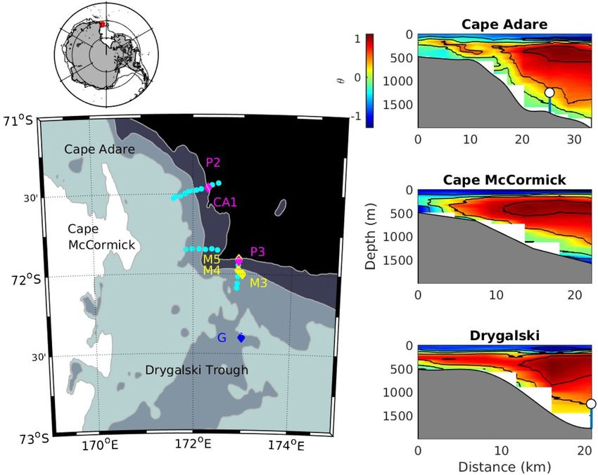
www.nature.com/scientificreports/
Figure 1. The study site is located on the western side of the Ross Sea (area of regional map shown in red on
the upper map). Moorings P2 and P3 were located on the 1750 m isobath off Cape Adare and near the Drygalski
Trough respectively (left panel; pink diamonds). The P2 mooring was deployed at the same location as the CA-1
mooring in the CALM experiment. The M3, M4 and M5 moorings were located near the Drygalski Trough
during the AnSlope experiment (yellow diamonds). Mooring G in the Drygalski Trough is part of the MORSea
Program (blue diamond). Contours are at 500 m, 1000 m, and 1750 m depth. Hydrographic sections were taken
in 2018 along three lines perpendicular to the slope (light blue dots). Potential temperatures from the three
sections are shown in the panels on the right, with the positions of the P2 and P3 moorings indicated. (Maps
produced in Matlab R2015a https://au.mathworks.com/products/matlab.html.).
of tidal velocities allows deep water renewal in some fjords27. We investigate how variations of tidal mixing may
control the export of bottom water from the Drygalski Trough using observations from moorings adjacent to
Cape Adare on the slope and in the Drygalski Trough and from hydrography. We first examine changes in the
bottom water between our measurements in 2018 and 2008–2010, when the Cape Adare Long-term Mooring
(CALM) experiment took place. We estimate the sources of bottom water at Cape Adare and show that two
annual pulses of cold water in 2018 have a contribution of HSSW from the Drygalski Trough. We then show that
much of the timing and magnitude of the dense water release from the trough can be related to the modulation
of the tidal velocities in the Ross Sea.
Results
Interannual and seasonal changes in bottom water at Cape Adare. The time series from the CALM
CA-1 and RSO-P2 moorings off Cape Adare show an increase in salinities over the bottom 500 m between 2008
and 2018 with the greatest increase near the bottom (Fig. 2). Salinity near bottom reaches a maximum in 2018
that is 0.04 greater than the maximum salinities measured from 2008 through 2010. Temperatures are similar
between the two time series. As a result, the average density of the water in the lower 500 m increased in 2018
compared to the earlier time series and there is a slight increase in the density difference between ~ 45 and
~ 470 m above the bottom.
The seasonal cycle near the sea floor at Cape Adare during 2018 is similar to the seasonal cycles observed
from 2008 through 2010. A maximum in salinity occurs around March and April coincident with low tempera-
tures (marked with A in Fig. 2). A second period of low temperatures occurs around October (indicated by B)
which is not accompanied by a change in salinities. The temperatures around October are particularly low in
2018 compared to 2008–2010.
Scientific Reports | (2021) 11:2246 | https://doi.org/10.1038/s41598-021-81793-5 2
Vol:.(1234567890)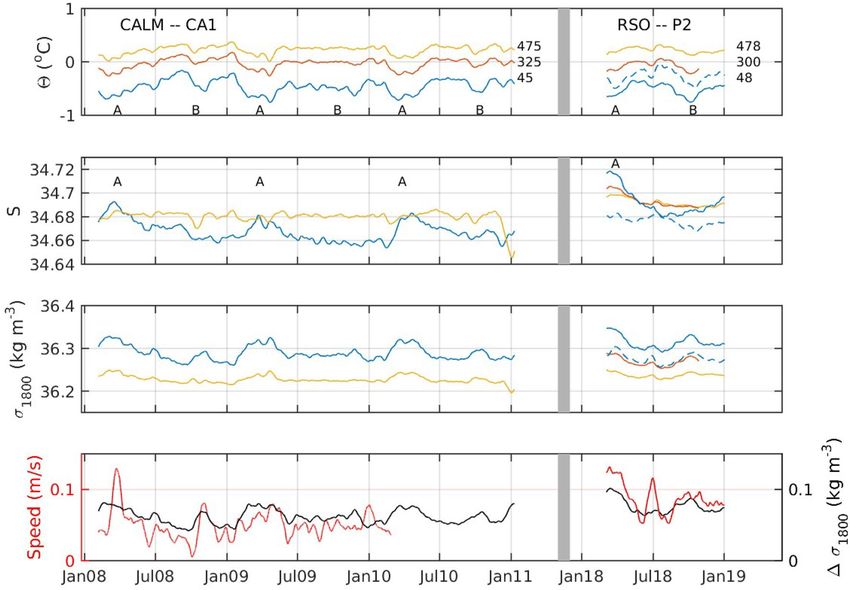
www.nature.com/scientificreports/
Figure 2. The potential temperature (top panel), salinity (second panel) and potential density at 1800 m
(third panel) at the location of the CALM CA-1 mooring and the RSO-P2 mooring. The grey line indicates
a discontinuity in time. Sensor height above bottom is shown next to the time series in the upper panel. The
letter ’A’ marks the cold, salty period every year between March and May. The letter ’B’ marks the second cold
period during October. The bottom panel shows the density difference between ~ 45 and ~ 475 m above bottom
(black line) and the speed of the current at ~ 475 m above bottom (red line). The dashed blue lines show the
water properties at the bottom sensor (48 m above bottom) at the RSO P3 mooring on a similar isobath near the
Drygalski Trough.
The RSO-P3 mooring, which is situated at a similar isobaths southeast of Cape Adare at the mouth of the
Drygalski Trough, measured water that is almost always warmer and less salty than that at Cape Adare (Fig. 2;
dashed blue lines). Water travelling along the isobath would take about a week to move between the P2 and P3
moorings, if it travels the average speed measured at the P3 mooring. However, the water at Cape Adare during
the two cold pulses in 2018 is too salty to be sourced from the water measured at P3, which is largely coming
from further east. We also note that times when cold, salty water is found at Cape Adare are when cold, salty
plumes arrive intermittently at P3 (Fig. 3), suggesting HSSW exiting the Drygalski Trough is responsible for
both cold periods at Cape Adare.
We investigated what proportion of water from the Drygalski Trough is needed to create the salinity and
temperature observed at Cape Adare every month during the RSO deployment (Fig. 4). We use the temperature
and salinity of CDW from the hydrography, HSSW properties from the mooring in the Drygalski T rough22 and
AABW from the water properties at the P3 mooring during each month (see Supplementary Table S1) with all
properties taken to the depth of the P2 sensor to find the proportions. The two cold pulses have a higher percent-
age of HSSW from the Ross Sea than the months before and after (34–36% for February/March and 22–23% for
September/October; Supplementary Table S2). The lowest percentages of HSSW occur between May and August
(10–18%) when the water properties at Cape Adare are most similar to the AABW coming from the east (esti-
mated as contributing 62–88% of the water at Cape Adare). The seasonal cycle in bottom water salinity at Cape
Adare can be explained by the higher salinity in the HSSW observed at Mooring G in the Drygalski Trough in
March22. The seasonal cycle in salinity suggests an approximately 8-month transit of dense water from formation
in the Terra Nova Bay polynya northward to the Drygalski Trough. As noted p reviously21, this time is consistent
flow speeds of ~ 0.025 m/s measured at Terra Nova Bay28 and the 450 km distance between them and with tracer
studies that suggest a transit time of less than a year29.
From the hydrographic survey, northward transport of AABW at Cape Adare in February 2018 is 0.5 Sv with
0.3 Sv at neutral densities γn > 28.27, which corresponds to 20% and 15%, respectively, of the total northward
transport of 2.7 Sv. The northward transport from the hydrographic section in 2004 calculated in the same man-
ner is greater: 1.6 Sv of AABW and 1.2 Sv for the higher neutral densities comprising 64% and 48%, respectively,
Scientific Reports | (2021) 11:2246 | https://doi.org/10.1038/s41598-021-81793-5 3
Vol.:(0123456789)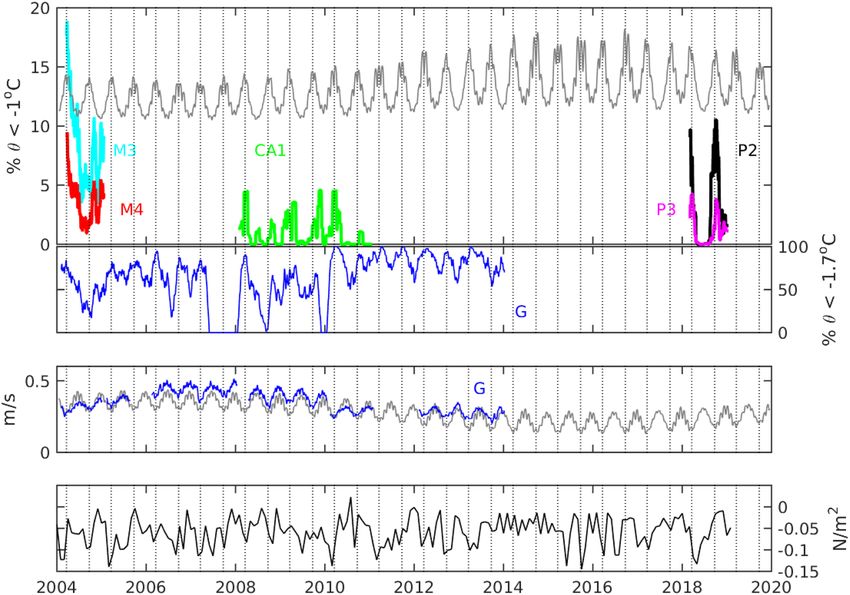
www.nature.com/scientificreports/
Figure 3. The top two panels show the hours per week that the lowest sensors on each mooring measured
water colder than − 1 °C (light blue bars) and also saltier than 34.75 (blue bars pointing downward). The red line
shows the cumulative total of plume events at P3 from 0 at the start of the record to 74 at the end. The speed of
the tidal flow at 478 m above bottom at P3 averaged over 3 days (black lines) is superimposed over the time of
cold water at both moorings. The lower three panels show the absolute value of the declination (|δ|) of the sun
(black) and moon (gray),
the
−1magnitude of the equilibrium tidal velocity averaged over 3 days and the inverse
averaged over a week ( ueq ).
Scientific Reports | (2021) 11:2246 | https://doi.org/10.1038/s41598-021-81793-5 4
Vol:.(1234567890)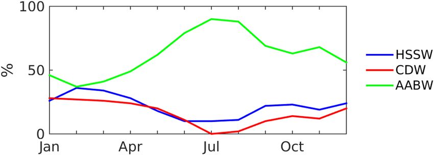
www.nature.com/scientificreports/
Figure 4. Percentage of water at the bottom sensor of the P2 mooring that can be attributed to HSSW from the
Ross Sea (blue), CDW (red) and AABW (green) from further east measured at the bottom sensor of P3.
of the total transport of 2.5 Sv. While the total transport estimates are similar, less dense water is observed at the
section in 2018 compared to the section in 2004.
Dense plumes from the Drygalski Trough. HSSW is measured intermittently at the P3 mooring, pri-
marily during March, when water less than − 1 °C and saltier than 34.75 is measured for several hours a week
(Fig. 3, top panel). A second period with similarly cold water, but fresher salinities, occurs during the last few
months of the year, with the greatest number of events during October. The events at the P3 mooring occur as
distinct plumes passing by the mooring with temperatures decreasing and salinities increasing over 20–60 min
and returning to their previous values within the next 4–10 h (see Supplementary Fig. S3). These plumes bring
dense water very rapidly (within a few hours) from the trough down the slope. We did not expect to see dense
plumes at this mooring: the M5 mooring during the AnSlope experiment was at a similar location and had
almost no instances where HSSW was measured. We would expect slightly denser plumes to travel further down
the slope, but we have no evidence that the water is more dense in 2018 than in 2004.
Cold water less than − 1 °C is also observed at the P2 mooring at Cape Adare during many of the same times
that plumes are present at the P3 mooring (Fig. 3, second panel). The two times when cold water appears at the
moorings are near the spring and autumn equinoxes when the solar declination is minimum and tidal velocities
are weaker (Fig. 3, third panel). However, there are other times when cold water appears periodically, particularly
from November through February after weak tidal velocities.
The correspondence between low tidal velocities and appearance of dense water suggests a reduction of tidal
mixing in the Drygalski Trough may allow dense water to escape. To investigate the potential tidal control, we
created tidal velocities using the timing of the cold periods at the mooring and the observed velocities at mooring
G in the Drygalski Trough. These reconstructed tidal velocities (Fig. 3, fourth panel) capture the weaker tides
during equinoxes. They also show spring-neap cycles with weaker velocities between November and February,
when the diurnal tides are counteracted by the low frequency tides and fewer periods of stronger tidal flow when
the two are acting together between May and October.
We examine a relationship between the tidal velocities and the outflow using the inverse of the tidal velocity.
Although this scaling approximates a linear drag law30,31, τ b = ρC D |utide |uout , the role of the non-linear terms
in the mean momentum balance may be c omplex17 and we do not attempt to account for it. Therefore, the scal-
ing should be regarded as a simple way to account for the regulation of the outflow by the tides and as a starting
point for future investigation. Using the inverse of the tidal velocity magnitude (Fig. 3, bottom panel) we find
cold water would be released in several pulses around the equinoxes and also in intermittent pulses when tidal
velocities are weak after the September equinox.
We used the RSO, CALM and AnSlope time series to further investigate the role of the wind and tides over
multiple years. Cold water appears at the bottom sensors of all the moorings in March and April with a second
period of cold water later in the year (Fig. 5). These periods of cold water measured at all the moorings often
line up with the equinoxes, when tidal energy due to the solar diurnal tides is minimum (Fig. 5, top panel), and
the alignment is particularly striking during the RSO experiment (P2 and P3). Tidal velocities at the Drygalski
Trough Mooring G also show clear minima at the equinoxes and the periods of low tidal energy correspond to
the presence of colder temperatures at the mooring (Fig. 5, second panel). The equilibrium tidal velocities (Fig. 5,
third panel, gray line) show the 18.6 years lunar declination cycle, increasing to major lunar standstill in 2006
followed by a decrease to minor lunar standstill, when the moon’s range of declinations is minimum in 2015.
The velocities at mooring G also show the cycle in lunar declination (Fig. 5, third panel, blue line). Strong veloci-
ties correspond with less cold water at the bottom-most sensor in the Drygalski Trough and weaker velocities
correspond with more cold water (Fig. 5, third and fourth panels). Some of this variation is likely due to sensor
placement, however vigorous tidal mixing is likely to be a factor setting the water properties of the HSSW exiting
the trough, with colder water leaving the trough when weaker tidal mixing reduces the amount of warmer CDW
being mixed into the dense water near the bottom.
We also take the inverse of the equilibrium tide to create a time series of expected release of dense water
from the Drygalski Trough (Fig. 5, grey line in the upper panel). The tidal velocities explain the release of dense
water at equinoxes as well as the increase in cold water during 2018 at P2 compared to the 2008–2011 CA1
Scientific Reports | (2021) 11:2246 | https://doi.org/10.1038/s41598-021-81793-5 5
Vol.:(0123456789)www.nature.com/scientificreports/
Figure 5. The upper panel shows the percentage of time water less than − 1 °C was measured at the bottom
sensor of each mooring every month. The gray line is |ueq|−1 with arbitrary offset and scaling. The second panel
shows the percentage of time water less than − 1.7 °C was measured at the bottom sensor of Mooring G in the
Drygalski Trough. The third panel shows the magnitude of the velocity, averaged over a month, at Mooring
G with the gray line showing the magnitude of u eq averaged over a month shifted downward by 0.15 m/s. The
bottom panel shows the along-slope wind stress in the central Ross Sea, where negative values indicate a greater
wind stress towards the west along the shelf. The vertical lines show the times of the equinoxes.
deployments. The reconstructed tide also reproduces the asymmetry in the occurrence of dense water between
the equinoxes: between the March and September equinoxes there is very little release of dense water because
the low frequency tide is adding to the diurnal tide, but between the September and March equinoxes there is a
“leakage” of dense water due to the low frequency tide periodically counteracting the diurnal tide and reducing
the velocity. These features are evident in the moored observations at Cape Adare, where both the P2 and CA1
moorings measure less cold water between March and September compared to the period between the September
and March equinoxes (Figs. 4 and 5).
Several of the characteristics of the dense water release cannot be explained by the tides. The AnSlope moor-
ings, M3 and M4, show the release of dense water on the March 2004 equinox, but a release of dense water after
the September equinox. Similarly, several peaks in the occurrence of cold water at CA-1 lag the minimum in
tidal velocity. It is possible that advection within the Ross Sea sets an additional time scale for the dense water
to move towards the shelf break after the tidal mixing weakens. It is also possible that other factors influence the
release of dense water through the year, such as the winds. We could find no correspondence between the local
wind stress near Cape Adare and the Drygalski Trough or the wind stress curl in the Ross Gyre. However, there
is a correspondence between cold water at the moorings and the along-slope wind stress in the central Ross Sea,
the region used to investigate the winds in the CALM experiment11 (Fig. 5, bottom panel). The correspondence
we find is for more cold water when along-slope winds are stronger in the direction of the polar easterlies, which
should tend to move the front onshore. This result is opposite to relationship found in the CALM study11 because
the wind products have changed markedly between our studies. The role of the winds and the potential interplay
of winds and tides on the outflow are questions deserving further study.
Discussion
The two co-located mooring deployments at Cape Adare show dense water appearing twice a year with highest
salinities measured in March. The analysis of water properties shows that both pulses of dense water near the
bottom at Cape Adare in 2018 can be explained as an increase in HSSW water from the Drygalski Trough. Using
rough22, the dense water at Cape Adare consists
the seasonal cycle in the salinity of HSSW from the Drygalski T
of 10–36% HSSW with two peaks, one in February/March and the other in September/October. When dense
Scientific Reports | (2021) 11:2246 | https://doi.org/10.1038/s41598-021-81793-5 6
Vol:.(1234567890)www.nature.com/scientificreports/
Distance above Potential
Mooring bottom (m) Salinity STD temperature (°C) STD Potential density STD Speed (m/s) STD
P2
− 71.4601 478 34.692 0.006 0.215 0.146 36.238 0.015
172.3024 477 0.13 0.07
1740 m 300 34.694 0.008 − 0.074 0.155 36.270 0.018
2018/2/19 177 No data
2019/1/17 48 34.693 0.015 − 0.513 0.226 36.314 0.027
20 0.47* 0.14*
P3
− 71.9181 453 34.697 0.005 0.412 0.141 36.219 0.013
172.9265 452 0.19 0.01
1715 m 301 34.651 0.007 0.177 0.189 36.236 0.017
2018/2/20 217 No data
2019/1/17 48 34.645 0.010 − 0.275 0.268 36.277 0.027
22 No data
Table 1. Instrumentation, depth, location and deployment dates for the P2 and P3 moorings. The mean and
standard deviation of properties from each sensor are given. Three instruments did not return data and the
lowest current meter on the P2 mooring collected data for only 1 month (denoted by an asterisk).
water is observed at Cape Adare, dense plumes of HSSW from the Drygalski Trough also appear at RSO-P3 on
the slope near the trough.
The pulses of dense water at Cape Adare during the RSO experiment are aligned with the equinoxes when
solar declination is minimum. A semi-annual variation was also noted in the appearance of dense water at Cape
Adare during the CALM e xperiment11. Plumes of dense water were most prevalent between November and May
during the AnSlope e xperiment9, with the spring-neap cycle also modulating the volume and properties of dense
water20. We find the diurnal and low frequency tides can explain the semi-annual occurrence of cold water at
Cape Adare as well as the bursts of dense water that appear between the September and March equinoxes. We
also suggest the 18.6 years modulation of lunar declination creates more pronounced pulses of dense water at
the equinoxes in 2018 compared to the equinoxes in 2008 through 2010. An inverse relationship with the tidal
velocity suggests the years around the lunar minimum in 2015 (and every 18.6 years) are the most favorable for
dense water outflow from the western Ross Sea. It is possible that the tides are also modulating the dense outflows
from the other troughs in the Ross Sea.
The increase in salinity off Cape Adare from 2008 to 2010–2018 is consistent with the observed changes in
water properties in the Ross Sea. Salinity decreased in the Drygalski Trough from 2008 until 2014, followed by
a more rapid increase from 2014 to 20187. The CALM observations show a slight decrease of salinity of 0.007/
year11, also consistent with the observations in the Ross Sea. The recent salinity increase has been linked to
increase in sea ice production in the Ross S ea32.
Water properties in the Ross Sea depend on the exchange of dense water flowing out with an inflow of CDW
across the slope. Simulations show ~ 50% of the CDW around the Antarctic crosses the slope into the Ross
Sea33. CDW is found far south in the Drygalski T rough21 and the appearance of CDW at Mooring G is strongly
22
modulated by the semi-annual tides . Simulations also show the inflow of CDW and outflow of dense water
are co-located in the troughs of the Ross Sea13,33. Therefore, export of dense water and the inflow of CDW are
dynamically linked, as regional process studies also suggest17. Here, we suggest tidal flows may be modulating the
exchange over a range of frequencies, as occurs in shallow systems34, in addition to internal hydraulic controls
found in deeper constrictions35. However, more work is needed to reconcile the scaling of bottom stress that we
have used with the more complex dependence of the outflow on the tides discussed in process simulations15,17.
Nevertheless, the regularity of the tides suggests we may be able to predict future exchange of CDW and HSSW
across the Ross Sea shelf break and estimate exchange in the past.
Methods
Ross sea outflow (RSO) experiment. A mooring (RSO-P2) was placed at Cape Adare (Fig. 1) from 19
February, 2018, to 17 January, 2019, in 1740 m of water to measure water properties and bottom water velocities
at the same location as the CA-1 mooring from the CALM study11. The mooring extended over the lower 478 m
of the water column and was instrumented with sensors at similar depths to the CALM mooring (Table 1) to
capture the benthic layer flow, extending the CALM time series. Another mooring (RSO-P3), with the same
configuration of instruments, was placed on a similar isobath on the slope north of the Drygalski Trough (Fig. 1
and Table 1) to measure water properties flowing towards Cape Adare from east of the Drygalski Trough.
Most sensors returned a complete time series. However, the batteries in the bottom current meters on both
moorings did not function properly: as a result, there are no near-bottom velocities at P3 and only during the
first deployment month at P2.
During the February 2018 voyage, three hydrographic sections were carried out perpendicular to the slope
(Fig. 1) to measure the temperature and salinity along the slope. The section off Cape Adare intersects the
Scientific Reports | (2021) 11:2246 | https://doi.org/10.1038/s41598-021-81793-5 7
Vol.:(0123456789)www.nature.com/scientificreports/
location of RSO-P2 and was completed first, followed by the section oriented nearly north to south at the mouth
of Drygalski Trough that contains the RSO-P3 mooring location. A third section was taken across the slope
near Cape McCormick. The deepest casts in this hydrographic section sampled a dense plume of HSSW from
the Drygalski Trough (Fig. 1 and see Supplementary Fig. S1). The plume was not present in the section further
south near the Drygalski Trough: it may be that the dense plume was not exiting the trough when the section
further south was completed a day earlier or it may be because the plume was exiting at shallower depths than
were measured in the section.
CALM, AnSlope and MORSea experiments. Moored observations from several previous experiments
were used in this study. The mooring CA-1 from the CALM experiment was deployed between January 2008
and January 2 01136. Measurements from this mooring were compared to those at RSO-P2 and consist of tem-
perature at 43 m, 298 m and 460 m above bottom, salinity at 43 m and 460 m, and velocity at 476 m above bot-
tom. Moored observations from the AnSlope experiment during 20049 were also used to examine the differences
in dense plumes between the RSO-P3 mooring and to investigate the timing of the dense plumes relative to the
tides. The temperature and salinity from the sensors 10 m above bottom on the M3 (691 m), M4 (984 m), and
M5 (1749 m) moorings were examined. Hydrographic data collected at Cape Adare in 2004 during the AnSlope
experiment was also compared to the hydrographic section collected in 2018.
The bottom water properties and flow within the Drygalski Trough were compared to the measurements on
the slope using the observations at the Marine Observatory of the Ross Sea (MORSea) mooring G maintained
over 10 years near 72.4° S, 173° E in ~ 520 m water depth22. Observations of temperature and velocity from 2004
to 2014 from the bottom-most sensors, which range in depth from 8 to 70 m above bottom, were used along
with salinity measured from 2005 through 2 00822 (see Supplementary Fig. S4).
Analysis of seasonal and interannual variability. To examine the seasonal and interannual variations
in water properties and currents, the moored observations from the RSO-P2 and CALM CA-1 moorings were
filtered over 31 days using a cosine filter. Blow down of the RSO-P2 mooring was minimal (98% of the time the
upper sensor was within 20 m of the minimum pressure and the lower sensors were within 6 m of the minimum
pressure). Therefore, we averaged the sensor data over the entire time period to obtain mean values. Averages
over the spring-neap cycle were performed with a 31-day cosine filter.
Identification of dense water at the moorings. Dense water is observed as short pulses at both moor-
ings, identified by a rapid decrease in temperature and increase in salinity, followed by a slower recovery to
background values. Cold plumes were identified in the moored records, following the AnSlope analysis9, by
finding any time with potential temperature less than − 1 °C. The presence of HSSW was identified when salinity
was greater than 34.75. The hours per week and per month these properties were present were also calculated
at each sensor.
Plume events were also identified as events when the difference between the maximum and minimum tem-
perature over any hour was greater than 0.5 °C and the minimum temperature was also less than − 1 °C. At the
RSO-P3 mooring there were 74 such instances (see Supplementary Fig. S3). At the RSO-P2 mooring, changes
in temperature were less sudden and tended to coincide with changes in the tidal velocity and, as a result, only
one event fit the definition.
Tidal analysis. To test whether cold water measured at the moorings at Cape Adare is released when tidal
velocities in the Drygalski Trough are weak, we examined the relationship between the occurrence of cold water
and the tides. The equilibrium tidal potential (ζ ) due to any celestial body has a low frequency component
(ζ0), a diurnal component (ζ1 ), and a semidiurnal component (ζ2 ) which can be related to known astronomical
variables37:
ζ = ζ0 + ζ1 + ζ2
mR4
3 sin2 θ − 1 3 sin2 δ − 1 + 3 sin 2θ sin 2δ cos � + 3 cos2 θ cos2 δ cos 2�
ζ = 3
4Mr
where the mass and radius of the Earth are M and R, the mass of the celestial body is m, the distance between
the Earth and the body is r, the latitude on the Earth is θ , the declination of the body is δ and is the changing
longitude due to the revolution of the Earth.
We calculated the solar and lunar equilibrium tides using ephemerides from Jet Propulsion Laboratory Hori-
zons Web-Interface38. At high latitudes, the semidiurnal component is small and varies little with declination; the
diurnal and low frequency equilibrium tides are much larger. In a channel, the tidal velocity is proportional to the
tidal potential but multiplied by factors due to propagation and r esonance39. We therefore constructed the tidal
velocity from the low frequency and diurnal components and found the coefficients that best fit the observations:
ζ0 ζ1
ueq = A +B 9 +C
109 10
where now the components ζ0 and ζ1 are the sum of the solar and lunar tidal potentials. We found the relation-
ship between A, B and C by finding the best fit to times when the velocity is near zero in the Drygalski Trough
mooring. We fit to times when ueq = 0 to simplify the fit and constrain it to times when mixing is weak. Taking
all times when the weekly average of the velocity magnitude is less than 0.2 m/s gives [A, B, C] = [0.71, − 1, 0.76].
Scientific Reports | (2021) 11:2246 | https://doi.org/10.1038/s41598-021-81793-5 8
Vol:.(1234567890)www.nature.com/scientificreports/
Adjusting the velocities for the different heights of the sensors using a log layer profile gives [A, B, C] = [0.87, − 1,
0.95]. We made an additional independent estimate by finding the best fit to times when cold water was most
prevalent at each mooring: we assume ueq = 0 for weeks when the number of cold hours is within 20% of the
maximum value at each mooring and found [A, B, C] = [1.16, − 1, 1.18] (see Supplementary Fig. S5).
Since the aim is to capture the main characteristics of the tides, we chose round numbers, [A, B, C] = [1, − 1,
1], and constructed the equilibrium tide, ueq, over the whole time period. We also compared the presence of cold
water at the moorings with the inverse of the tidal velocity, |ueq |−1, which we used as a scale for the reduction of
bottom drag and potential release of HSSW from the Drygalski Trough.
Wind analysis. We investigated whether variability of the regional winds may be related to flow and water
properties from the moored observations using monthly mean wind stress from the Fifth generation of the
European Centre for Medium-Range Weather Forecasts atmospheric reanalysis (ERA-5, 1/4° × 1/4° resolution).
We averaged wind stress over the same region used in the CALM experiment, 70°–75° S and 175° E–175° W,
and rotated the coordinate system 40° to follow the direction of the slope in the central Ross Sea at 1 75oW as
done previously11. We also examined the wind stress curl and averaged it over the Ross Gyre region from 170°E
to 130°W and 65°–75° S, and examined local wind stress along the slope at both the Drygalski Trough and Cape
Adare.
Transport from hydrography. The along-slope transports were calculated from the hydrographic sec-
tions in February 2018. Dynamic heights were calculated from temperature and salinity profiles (Fig. 1 and
see Supplementary Figs. S1 and S2) and geostrophic shear estimated between each pair of profiles across each
section. A mean dynamic topography (CLS-CNES2013)40 was interpolated to the location of each profile and
the surface geostrophic velocity calculated between each profile and added to the shear from the hydrography
to obtain the total geostrophic velocity. The velocities were then integrated within density ranges to find the
transport of dense water. We used neutral densities greater than 28.27 to define the dense water associated with
Ross Sea bottom water. We also found the transport of AABW by integrating velocities of water with properties
between − 0.75 < θ < 0.24 and 34.68 < S < 34.7241,42 in depths over 1000 m. The along-slope transport was calcu-
lated in the same way from an identical section at Cape Adare collected in March, 2004.
Data availability
The hydrographic data are available on the World Ocean Database and the moored data from the MORSea
Project website.
Received: 10 August 2020; Accepted: 7 January 2021
References
1. Johnson, G. C. Quantifying Antarctic bottom water and North Atlantic deep water volumes. J. Geophys. Res. https://doi.
org/10.1029/2007JC004477 (2008).
2. Orsi, A. H. On the total input of Antarctic waters to the deep ocean: A preliminary estimate from chlorofluorocarbon measure-
ments. J. Geophys. Res. https://doi.org/10.1029/2001JC000976 (2002).
3. Purkey, S. G. & Johnson, G. C. Global contraction of Antarctic bottom water between the 1980s and 2000s*. J. Clim. 25, 5830–5844.
https://doi.org/10.1175/JCLI-D-11-00612.1 (2012).
4. Purkey, S. G. & Johnson, G. C. Antarctic bottom water warming and freshening: Contributions to sea level rise, ocean freshwater
budgets, and global heat gain*. J. Clim. 26, 6105–6122. https://doi.org/10.1175/JCLI-D-12-00834.1 (2013).
5. van Wijk, E. M. & Rintoul, S. R. Freshening drives contraction of Antarctic Bottom Water in the Australian Antarctic Basin.
Geophys. Res. Lett. 41, 1657–1664. https://doi.org/10.1002/2013GL058921 (2014).
6. Jacobs, S. S. & Giulivi, C. F. Large multidecadal salinity trends near the Pacific-Antarctic Continental Margin. J. Clim. 23, 4508–
4524. https://doi.org/10.1175/2010JCLI3284.1 (2010).
7. Castagno, P. et al. Rebound of shelf water salinity in the Ross Sea. Nat. Commun. https://doi.org/10.1038/s41467-019-13083-8
(2019).
8. Bergamasco, A., Defendi, V., Zambianchi, E. & Spezie, G. Evidence of dense water overflow on the Ross Sea shelf-break. Antarct.
Sci. 14, 271–277. https://doi.org/10.1017/S0954102002000068 (2002).
9. Gordon, A. L. et al. Western Ross Sea continental slope gravity currents. Deep Sea Res. Part II Trop. Stud. Oceanogr. 56, 796–817.
https://doi.org/10.1016/j.dsr2.2008.10.037 (2009).
10. Baines, P. G. A model for the structure of the Antarctic Slope Front. Deep Sea Res. Part II Trop. Stud. Oceanogr. 56, 859–873. https
://doi.org/10.1016/j.dsr2.2008.10.030 (2009).
11. Gordon, A. L., Huber, B. A. & Busecke, J. Bottom water export from the western Ross Sea, 2007 through 2010. Geophys. Res. Lett.
42, 5387–5394. https://doi.org/10.1002/2015GL064457 (2015).
12. Gordon, A. L., Huber, B., McKee, D. & Visbeck, M. A seasonal cycle in the export of bottom water from the Weddell Sea. Nat.
Geosci. 3, 551–556. https://doi.org/10.1038/ngeo916 (2010).
13. Dinniman, M. S., Klinck, J. M. & Smith, W. O. A model study of Circumpolar Deep Water on the West Antarctic Peninsula and
Ross Sea continental shelves. Deep Sea Res. Part II Trop. Stud. Oceanogr. 58, 1508–1523. https: //doi.org/10.1016/j.dsr2.2010.11.013
(2011).
14. Stewart, A. L. & Thompson, A. F. Eddy-mediated transport of warm Circumpolar Deep Water across the Antarctic Shelf Break.
Geophys. Res. Lett. 42, 432–440. https://doi.org/10.1002/2014GL062281 (2015).
15. Muench, R., Padman, L., Gordon, A. & Orsi, A. A dense water outflow from the Ross Sea, Antarctica: Mixing and the contribution
of tides. J. Mar. Syst. 77, 369–387. https://doi.org/10.1016/j.jmarsys.2008.11.003 (2009).
16. Robertson, R. Tidally induced increases in melting of Amundsen Sea ice shelves. J. Geophys. Res. Oceans 118, 3138–3145. https://
doi.org/10.1002/jgrc.20236(2013).
17. Wang, Q. et al. Enhanced cross-shelf exchange by tides in the western Ross Sea. Geophys. Res. Lett. 40, 5735–5739. https://doi.
org/10.1002/2013GL058207 (2013).
Scientific Reports | (2021) 11:2246 | https://doi.org/10.1038/s41598-021-81793-5 9
Vol.:(0123456789)www.nature.com/scientificreports/
18. Jendersie, S., Williams, M. J. M., Langhorne, P. J. & Robertson, R. The density-driven winter intensification of the ross sea circula-
tion. J. Geophys. Res. Oceans 123, 7702–7724. https://doi.org/10.1029/2018JC013965 (2018).
19. Robertson, R. Baroclinic and barotropic tides in the Ross Sea. Antarct. Sci. 17, 107–120 (2005).
20. Padman, L., Howard, S. L., Orsi, A. H. & Muench, R. D. Tides of the northwestern Ross Sea and their impact on dense outflows
of Antarctic Bottom Water. Deep Sea Res. Part II Trop. Stud. Oceanogr. 56, 818–834. https://doi.org/10.1016/j.dsr2.2008.10.026
(2009).
21. Budillon, G., Castagno, P., Aliani, S., Spezie, G. & Padman, L. Thermohaline variability and Antarctic bottom water formation at
the Ross Sea shelf break. Deep Sea Res. Part I Oceanogr. Res. Papers 58, 1002–1018 (2011).
22. Castagno, P., Falco, P., Dinniman, M. S., Spezie, G. & Budillon, G. Temporal variability of the Circumpolar Deep Water inflow
onto the Ross Sea continental shelf. J. Mar. Syst. 166, 37–49. https://doi.org/10.1016/j.jmarsys.2016.05.006 (2017).
23. Ou, H.-W., Guan, X. & Chen, D. Tidal effect on the dense water discharge, Part 1: Analytical model. Deep Sea Res. Part II Topical
Stud. Oceanogr. 56, 874–883. https://doi.org/10.1016/j.dsr2.2008.10.031 (2009).
24. Guan, X., Ou, H.-W. & Chen, D. Tidal effect on the dense water discharge, Part 2: A numerical study. Deep Sea Res. Part II Topical
Stud. Oceanogr. 56, 884–894. https://doi.org/10.1016/j.dsr2.2008.10.028 (2009).
25. Bowen, M. M. & Geyer, W. R. Salt transport and the time-dependent salt balance of a partially stratified estuary. J. Geophys. Res.
https://doi.org/10.1029/2001JC001231 (2003).
26. Nunes, R. A. & Lennon, G. W. Episodic stratification and gravity currents in a marine environment of modulated turbulence. J.
Geophys. Res. Oceans 92, 5465–5480. https://doi.org/10.1029/JC092iC05p05465 (1987).
27. Cannon, G. A., Holbrook, J. R. & Pashinski, D. J. Variations in the onset of bottom-water intrusions over the entrance sill of a fjord.
Estuaries 13, 31–42. https://doi.org/10.2307/1351430 (1990).
28. Fusco, G., Budillon, G. & Spezie, G. Surface heat fluxes and thermohaline variability in the Ross Sea and in Terra Nova Bay polynya.
Cont. Shelf Res. 29, 1887–1895. https://doi.org/10.1016/j.csr.2009.07.006 (2009).
29. Rivaro, P., Frache, R., Bergamasco, A. & Hohmann, R. Dissolved Oxygen, NO and PO as tracers for Ross Sea Ice Shelf Water
overflow. Antarct. Sci. 15, 399–404. https://doi.org/10.1017/S095410200300141X (2003).
30. Lentz, S. J. & Fewings, M. R. The Wind- and wave-driven inner-shelf circulation. Annu. Rev. Mar. Sci. 4, 317–343. https://doi.
org/10.1146/annurev-marine-120709-142745 (2012).
31. LaCasce, J. H. & Isachsen, P. E. The linear models of the ACC. Prog. Oceanogr. 84, 139–157. https://doi.org/10.1016/j.pocea
n.2009.11.002 (2010).
32. Silvano, A. et al. Recent recovery of Antarctic Bottom Water formation in the Ross Sea driven by climate anomalies. Nat. Geosci.
https://doi.org/10.1038/s41561-020-00655-3 (2020).
33. Morrison, A. K., Hogg, A. M., England, M. H. & Spence, P. Warm Circumpolar Deep Water transport toward Antarctica driven
by local dense water export in canyons. Sci. Adv. 6, eaav2516. https://doi.org/10.1126/sciadv.aav2516 (2020).
34. Linden, P. F. & Simpson, J. E. Modulated mixing and frontogenesis in shallow seas and estuaries. Cont. Shelf Res. 8, 1107–1127.
https://doi.org/10.1016/0278-4343(88)90015-5 (1988).
35. Farmer, D. M. & Armi, L. The flow of Atlantic water through the Strait of Gibraltar. Prog. Oceanogr. 21, 1–103. https://doi.
org/10.1016/0079-6611(88)90055-9 (1988).
36. Huber, B. & Gordon, A. Processed currentmeter data from the adare basin near antarctica acquired during the nathaniel B. Palmer
expedition NBP1101 (2011). https://doi.org/10.1594/IEDA/321392 (2015).
37. Godin, G. The analysis of tides (Toronto University Press, 1972).
38. JPL HORIZONS. Web-interface on-line solar system data and ephermis computation service. https://ssd.jpl.nasa.gov/horizons.
cgi (2020).
39. Gill, A. E. Atmosphere-Ocean Dynamics (Academic Press, London, 1982).
40. Rio, M. H., Mulet, S. & Picot, N. Beyond GOCE for the ocean circulation estimate: Synergetic use of altimetry, gravimetry,
and in situ data provides new insight into geostrophic and Ekman currents. Geophys. Res. Lett. 41, 8918–8925. https://doi.
org/10.1002/2014GL061773 (2014).
41. Orsi, A. H., Johnson, G. C. & Bullister, J. L. Circulation, mixing, and production of Antarctic Bottom Water. Prog. Oceanogr. 43,
55–109. https://doi.org/10.1016/S0079-6611(99)00004-X (1999).
42. Orsi, A. H. & Wiederwohl, C. L. A recount of Ross Sea waters. Deep Sea Res. Part II Topical Stud. Oceanogr. 56, 778–795. https://
doi.org/10.1016/j.dsr2.2008.10.033 (2009).
Acknowledgements
We would like to thank Sarah Searson, Olivia Price, Matt Walkington, David Bowden, Richard O’Driscoll, and
the captain and crew of the R.V. Tangaroa. M.B., D.F. and A.F.-V. were supported by the Deep South National Sci-
ence Challenge with additional support from the University of Auckland and the New Zealand Strategic Science
Investment Fund: Antarctic Science Platform Contract ANTA1801. This is Lamont-Doherty Earth Observatory
contribution 8465. The mooring G data were collected in the framework of MORSea projects supported by the
Italian National Program for Antarctic Research‐PNRA, which provided financial and logistic support. PC was
funded by the PNRA, Grant PNRA18_00256. The PNRA is funded by Italian Minister of the University.
Author contributions
M.B., D.F. and A.F.-V. conceived of the study. A.F.-V. conducted the field work. M.B. performed the analysis
of the moored observations, led the writing, and created the figures. D.F. analysed the hydrographic and wind
observations. A.G., B.H., P.C. and P.F. advised on analysis and interpretation. All authors reviewed and contrib-
uted to the manuscript.
Funding
This study was funded by the New Zealand Ministry of Business Innovation and Employment through the Deep
South National Science Challenge.
Competing interests
The authors declare no competing interests.
Additional information
Supplementary Information The online version contains supplementary material available at https://doi.
org/10.1038/s41598-021-81793-5.
Scientific Reports | (2021) 11:2246 | https://doi.org/10.1038/s41598-021-81793-5 10
Vol:.(1234567890)www.nature.com/scientificreports/
Correspondence and requests for materials should be addressed to M.M.B.
Reprints and permissions information is available at www.nature.com/reprints.
Publisher’s note Springer Nature remains neutral with regard to jurisdictional claims in published maps and
institutional affiliations.
Open Access This article is licensed under a Creative Commons Attribution 4.0 International
License, which permits use, sharing, adaptation, distribution and reproduction in any medium or
format, as long as you give appropriate credit to the original author(s) and the source, provide a link to the
Creative Commons licence, and indicate if changes were made. The images or other third party material in this
article are included in the article’s Creative Commons licence, unless indicated otherwise in a credit line to the
material. If material is not included in the article’s Creative Commons licence and your intended use is not
permitted by statutory regulation or exceeds the permitted use, you will need to obtain permission directly from
the copyright holder. To view a copy of this licence, visit http://creativecommons.org/licenses/by/4.0/.
© The Author(s) 2021
Scientific Reports | (2021) 11:2246 | https://doi.org/10.1038/s41598-021-81793-5 11
Vol.:(0123456789)You can also read