The SAMI Galaxy Survey: the third and final data release - arXiv

MNRAS 000, 1–27 (2021) Preprint 1 February 2021 Compiled using MNRAS LATEX style file v3.0

 The SAMI Galaxy Survey: the third and final data release

 Scott M. Croom1,2★ , Matt S. Owers3,4 , Nicholas Scott1,2 , Henry Poetrodjojo1,2 ,
 Brent Groves5,6,2 , Jesse van de Sande1,2 , Tania M. Barone6,1,2 , Luca Cortese5,2 ,
 Francesco D’Eugenio7 , Joss Bland-Hawthorn1,2 , Julia Bryant1,2 , Sree Oh6,2 ,
 Sarah Brough8,2 , James Agostino9 , Sarah Casura10 , Barbara Catinella5,2 ,
 Matthew Colless6,2 , Gerald Cecil11 , Roger L. Davies12 , Michael J. Drinkwater13 ,
arXiv:2101.12224v1 [astro-ph.GA] 28 Jan 2021

 Simon P. Driver5 , Ignacio Ferreras14,15,16 , Caroline Foster1,2 , Amelia Fraser-McKelvie5,2 ,
 Jon Lawrence17 , Sarah K. Leslie18,2 , Jochen Liske10 , Ángel R. López-Sánchez3,4,2 ,
 Nuria P. F. Lorente17 , Rebecca McElroy1,2 , Anne M. Medling9,2 , Danail Obreschkow5,2 ,
 Samuel N. Richards19 , Rob Sharp6 , Sarah M. Sweet12,2 , Dan S. Taranu20 ,
 Edward N. Taylor21 , Edoardo Tescari22 , Adam D. Thomas6,2 , James Tocknell17 ,
 Sam P. Vaughan 1,2
 1 Sydney Institute for Astronomy (SIfA), School of Physics, The University of Sydney, NSW, 2006, Australia
 2 ARC Centre of Excellence for All Sky Astrophysics in 3 Dimensions (ASTRO 3D)
 3 Department of Physics and Astronomy, Macquarie University, NSW, 2109, Australia
 4 Astronomy, Astrophysics and Astrophotonics Research Centre, Macquarie University, Sydney, NSW 2109, Australia
 5 ICRAR, The University of Western Australia, Crawley WA 6009, Australia
 6 Research School of Astronomy and Astrophysics, Australian National University, Canberra, ACT 2611, Australia
 7 Sterrenkundig Observatorium, Universiteit Gent, Krijgslaan 281 S9, B-9000 Gent, Belgium
 8 School of Physics, University of New South Wales, NSW 2052, Australia
 9 Ritter Astrophysical Research Center, University of Toledo, Mail Stop 111, Toledo, OH, 43606, United States
 10 Hamburger Sternwarte, Universität Hamburg, Gojenbergsweg 112, 21029 Hamburg, Germany
 11 Dept. Physics and Astronomy University of North Carolina Chapel Hill, NC 27599 USA
 12 Astrophysics, Department of Physics, University of Oxford, Denys Wilkinson Building, Keble Rd., Oxford, OX1 3RH, UK.
 13 School of Mathematics and Physics, University of Queensland, Brisbane, QLD 4072, Australia
 14 Department of Physics and Astronomy, University College London, Gower Street, London WC1E 6BT, UK
 15 Instituto de Astrofisica de Canarias, Calle Via Lactea s/n, E38205 La Laguna, Tenerife, Spain
 16 Departamento de Astrofisica, Universidad de La Laguna (ULL), La Laguna, E-38206 Tenerife, Spain
 17 Australian Astronomical Optics - Macquarie, Macquarie University, NSW 2109, Australia
 18 Leiden Observatory, Leiden University, PO Box 9513, NL-2300 RA Leiden, the Netherlands
 19 SOFIA Science Center, USRA, NASA Ames Research Center, Building N232, M/S 232-12, P.O. Box 1, Moffett Field, CA 94035-0001, USA
 20 Department of Astrophysical Sciences, Princeton University, 4 Ivy Lane, Princeton, NJ 08544, USA
 21 Centre for Astrophysics and Supercomputing, Swinburne University of Technology, John Street, Hawthorn, VIC 3122, Australia
 22 Melbourne Data Analytics Platform (MDAP), The University of Melbourne, Parkville, VIC 3010, Australia

 Accepted XXX. Received YYY; in original form ZZZ

 ABSTRACT
 We have entered a new era where integral-field spectroscopic surveys of galaxies are sufficiently
 large to adequately sample large-scale structure over a cosmologically significant volume. This
 was the primary design goal of the SAMI Galaxy Survey. Here, in Data Release 3 (DR3), we
 release data for the full sample of 3068 unique galaxies observed. This includes the SAMI
 cluster sample of 888 unique galaxies for the first time. For each galaxy, there are two primary
 spectral cubes covering the blue (370–570 nm) and red (630–740 nm) optical wavelength
 ranges at spectral resolving power of = 1808 and 4304 respectively. For each primary cube,
 we also provide three spatially binned spectral cubes and a set of standardized aperture spectra.
 For each galaxy, we include complete 2D maps from parameterized fitting to the emission-line
 and absorption-line spectral data. These maps provide information on the gas ionization and
 kinematics, stellar kinematics and populations, and more. All data are available online through
 Australian Astronomical Optics (AAO) Data Central.
 Key words: galaxies: general – galaxies: kinematics and dynamics – galaxies: star formation
 © 2021 The Authors – galaxies: stellar content – galaxies: clusters: general – astronomical data bases: surveys.

2 S. M. Croom et al.
1 INTRODUCTION plex multi-parameter nature of galaxy formation drives us to much
 larger samples, which motivated the step to multi-object integral
Our understanding of how galaxies form and evolve has taken great field spectrographs. The SAMI Galaxy Survey (Croom et al. 2012;
strides in the last few decades, but we are far from a complete picture. Bryant et al. 2015) was the first of these large-scale multiplexed
No two galaxies are the same, as illustrated by many attempts to find projects, followed by MaNGA (Bundy et al. 2015). Future projects
close analogues of the Milky Way or M31 (e.g. Bland-Hawthorn & such as Hector (Bryant et al. 2016) will further extend the reach of
Gerhard 2016; Boardman et al. 2020). This complexity is apparent integral-field spectroscopic surveys.
in the range of distinct components within galaxies, e.g. truncated or
extended dark matter haloes, one or more disks, long bars and rings, The SAMI Galaxy Survey (Croom et al. 2012; Bryant et al.
short bars/bulges, smooth or structured stellar bulges and haloes, 2015) aimed to span the plane of mass and environment with a large
central star clusters and nuclear disks, or a massive black hole, sample of galaxies, each with spatially-resolved structural and kine-
as well as different gas/dust (molecular, atomic, ionized) phases. matic measurements. The specific science goals for the survey were
To further complicate matters, the different components or phases to answer the questions i) what is the physical role of environment
interact in a variety of ways: gas cooling to form stars, stellar or in galaxy evolution? ii) What is the interplay between gas flows and
supernovae feedback, feedback from a central super-massive black galaxy evolution? iii) How are mass and angular momentum built
hole, dynamical mixing from bars, etc. It is a daunting task to form up in galaxies? As part of this we aimed to compare and contrast our
a coherent narrative for all of these processes over cosmic time, and 3D integral field data cubes for each galaxy with synthetic galaxies
to demonstrate the robustness of this narrative with a consistent set emerging from cosmological simulations sampled in the same fash-
of cosmological simulations. Yet only when this is achieved can ion. Our first detailed comparisons reveal that all simulators are able
we begin to claim a solid understanding of the primary processes to match a subset of the galaxy parameters, but often at the expense
involved in a galaxy’s life cycle. of other parameters (van de Sande et al. 2019). The inconsistencies
 In recent years, questions have been raised about the limita- are due largely to our limited understanding of the many complex
tions of finite resolution in cosmological simulations, as well as baryonic processes that work together over billions of years.
chaotic-like behaviour — the ‘butterfly effect’ — particularly in The SAMI Galaxy Survey observations took place between
relation to the inherent complexity of so many competing processes 2013 and 2018, obtaining data for over 3000 galaxies. These data
and whether we will ever be able to track these interactions mean- have been used in a wide variety of scientific analyses, including
ingfully (Genel et al. 2019; Keller et al. 2019; Keller & Kruijssen studies of galactic winds (Fogarty et al. 2012; Ho et al. 2014, 2016b),
2020). To make robust tests of these simulations requires us to ac- the relationship of angular momentum and spin to galaxy properties
quire observations with sufficient information on each galaxy. Cou- and environment (Fogarty et al. 2014; Cortese et al. 2016; van de
pled with this, we need to sample galaxies over a cosmologically Sande et al. 2017b; Brough et al. 2017; Foster et al. 2017; Welker
representative volume. et al. 2020), stellar populations (Scott et al. 2017; Barone et al.
 We know that mass is a fundamental parameter in controlling 2018; Ferreras et al. 2019; Santucci et al. 2020), star formation
galaxy properties. For example, star formation, mean stellar age and and quenching (Medling et al. 2018; Schaefer et al. 2019; Owers
morphology are strongly linked to stellar mass (e.g. Baldry et al. et al. 2019; Cortese et al. 2019; Varidel et al. 2020), gas-phase
2006). We also now understand that a galaxy’s life is shaped by its metallicity, (Poetrodjojo et al. 2018; Sánchez et al. 2019) kinematic
surroundings. Environment is known to modify galaxy morphology and structural scaling relations (Cortese et al. 2014; Bloom et al.
(e.g. Dressler 1980), current star formation (e.g. Lewis et al. 2002) 2017; Barat et al. 2019; Oh et al. 2020), detailed comparison to
and star formation history (e.g. Blanton & Moustakas 2009). In simulations (van de Sande et al. 2019; Khim et al. 2020), and much
some cases it appears that the trends in mass and environment may more. The SAMI Galaxy Survey team have provided regular data
be separable (e.g. Peng et al. 2010). releases (Allen et al. 2015; Green et al. 2018; Scott et al. 2018). In
 Other properties of galaxies also have important evolutionary this current paper we present the third and final data release (DR3)
roles, such as angular momentum, binding energy, gas and dark of all SAMI observations, together with value-added products such
matter fractions. A challenge for us is to separate the trends in the as stellar kinematics, stellar populations and emission line fits. This
driving parameters from stochastic effects. In the fullness of time, is the first SAMI data release to contain data from the eight massive
it may even be possible to reveal the drivers behind apparently galaxy clusters observed as part of the SAMI Galaxy Survey. We
stochastic evolution, for example, uncovering the detailed merger also include for the first time environmental metrics for the entire
history of a galaxy. However, for now we often have to average SAMI sample.
over the stochasticity, and this is one of the requirements that drives In Section 2 we outline the survey input catalogues, the instru-
us to large samples of galaxies. To complicate matters further, we ment and the observations. In Section 3 we discuss improvements in
observe galaxies over a randomized distribution of viewing angles. data reduction and assessments of data quality. Section 4 describes
This also pushes us to larger samples in order to determine internal the primary data products from the survey, including cubes (with
properties from projected properties. various binning schemes) and aperture spectra. Catalogues based
 The requirement for larger samples has driven the large-scale on photometric data of SAMI targets are discussed in Section 5. The
multi-fibre spectroscopic surveys of the last two decades (York et al. stellar kinematics and stellar population products are discussed in
2000; Colless et al. 2001; Driver et al. 2011), that have character- Sections 6 and 7 respectively. Emission line products are presented
ized the local galaxy distribution very effectively. However, the in Section 8. In Section 9 we discuss environmental metrics within
need to understand the internal structure of galaxies has driven the the SAMI Galaxy Survey. Discussion of data access is provided in
development of integral-field spectroscopic surveys. This was pio- Section 10 and we summarize the paper in Section 11. Throughout
neered by the SAURON project (Bacon et al. 2001) and followed the paper we assume a cosmology with Ωm = 0.3, ΩΛ = 0.7 and
by ATLAS3D (Cappellari et al. 2011), both focussed on early-type 0 = 70 km s−1 Mpc−1 . All magnitudes are in the AB system (Oke
galaxies. The CALIFA survey was the first to cover a large number & Gunn 1983) and stellar masses and star-formation rates assume a
(∼ 600) of galaxies of all types (Sánchez et al. 2012). The com- Chabrier IMF (Chabrier 2003).

 MNRAS 000, 1–27 (2021)

The SAMI Galaxy Survey: DR3 3

Table 1. The coordinates and number of objects in the GAMA regions. For each region we list the right ascension (RA) and declination (Dec.). For both the
primary and secondary samples we list the number of observed galaxies obs , the number of good targets good (i.e. those not flagged as bad for photometric
reasons such as a bright star in the field-of-view) and the number of all targets all (including objects with bad flags). The listed completeness for the primary
sample is obs / good .

 Region RA (J2000) Dec. (J2000) Primary Secondary Primary
 deg deg obs / good / all obs / good / all Completeness

 GAMA 09h 129.0 to 141.0 −1 to +3 575/683/806 82/699/820 84.2%
 GAMA 12h 174.0 to 186.0 −2 to +2 637/728/805 65/900/982 87.5%
 GAMA 15h 211.5 to 223.5 −2 to +2 728/995/1127 13/915/996 73.2%

 Total 1940/2406/2738 160/2514/2798 80.6%

2 THE SAMI GALAXY SURVEY (0.6 percent of the input catalogue). This was typically in order to
 place an asymmetric galaxy or a close pair fully into the integral
2.1 The Input Catalogues
 field unit (IFU) and these objects have BAD_CLASS=5. The input
The input catalogues used for the SAMI Galaxy Survey are drawn catalogue that is publicly available as part of DR3 contains both
from the three equatorial regions of the Galaxy And Mass Assembly object coordinates and IFU pointing coordinates. 88.8 percent of
(GAMA) Survey (Driver et al. 2011), as described in Bryant et al. the input catalogue remained as a target after flagging for problems.
(2015), and eight cluster regions described in Owers et al. (2017). In These good objects to be observed had either BAD_CLASS=0 or
addition, a small number of observations were made of filler targets 5. A further case of BAD_CLASS=8 is also included in observa-
when not all the integral field units could be allocated to main survey tions, but only the cluster regions contain galaxies with these values.
targets. We describe the different input catalogues below. BAD_CLASS=8 indicates a galaxy that is the smaller component
 of a close pair, where the more massive galaxy is outside of the
 field of view of the IFU. The full GAMA region input sample is
2.1.1 GAMA regions contained within the InputCatGAMADR3 catalogue.
The majority of galaxies in the SAMI Galaxy Survey are within A calibration star was observed in one IFU during every galaxy
regions observed as part of the GAMA survey. This provides the observation. This star allowed improved flux calibration and a good
substantial advantage of deep and complete spectroscopic coverage estimate of the spatial point spread function (PSF). These calibration
to select targets and define environment. The GAMA regions also stars were selected to be F-stars, based on their SDSS photometric
contain excellent photometric data across 21 bands from ultraviolet properties. Bryant et al. (2015) describes the selection of calibration
to far-infrared (Driver et al. 2016). Bryant et al. (2015) describe stars in detail. The catalogue of calibration stars is released as part
the selection of targets in the GAMA regions in detail, but for of DR3 and called FstarCatGAMA.
completeness we outline the selection here.
 The SAMI Galaxy Survey targets in the GAMA regions were
selected within three 4 × 12 degree regions along the equator (dec- 2.1.2 Cluster regions
lination ' 0 degrees), centred at approximate right ascension (RA)
of 9, 12 and 15 hours (see Table 1). Galaxies were targeted based on The cluster targets were drawn from eight regions centred at the
cuts in the redshift-stellar mass plane, with a stellar mass proxy that positions listed in Table 2. Photometry was based either on SDSS
used -band magnitude and − colour (Taylor et al. 2011; Bryant DR9 (Ahn et al. 2012) or the VLT Survey Telescope ATLAS Survey
et al. 2015). Galaxies were selected within a series of four stepped (Shanks et al. 2015), with details of the selection described by
volumes, with higher stellar mass limits at higher redshift (see Fig. Owers et al. (2017). Targets were selected to be within a redshift
4 of Bryant et al. 2015). The primary sample is limited to redshift range defined by the relative velocity of the galaxy with respect to
 < 0.095. Observations aimed to have high and uniform complete- the cluster redshift, clus , such that | pec |/ 200 < 3.5. pec is the
ness for this primary sample. A secondary sample was also defined peculiar velocity of the galaxy with respect to the cluster redshift
that included high mass galaxies to higher redshift ( < 0.115) and and 200 is the velocity dispersion of the cluster of interest measured
used fainter stellar mass limits. As the secondary targets were ob- within the over-density radius 200 [see Section 9.2 and Owers et al.
served at lower priority, these are less complete (see Table 1). Fig. (2017) for further details]. We note that this cut in redshift is less
1 shows the distribution of primary (observed: red, unobserved: conservative than the criterion used to allocate cluster membership
blue) and secondary targets (observed: magenta, unobserved: cyan) in Owers et al. (2017), and so the input catalogue contains galaxies
in redshift and RA. A set of filler galaxies, at lower priority that the that are close to the cluster in redshift space, but may not be bona-
secondary targets, was also defined. These are discussed in Section fide members.
2.1.3. In addition to meeting the aforementioned criteria, targets were
 Each potential target was visually checked to identify prob- further characterised into primary and secondary targets. Primary
lems, such as bright nearby stars or sources being a sub-component targets are defined as those that meet the following:
of a larger galaxy. These were flagged within the input catalogue and • Cluster-centric distance < 200 ,
their priority set so that they were not observed. The column named • for 0.045 < clus < 0.06, stellar mass ∗ > 1010 M ,
BAD_CLASS in the input catalogue (named InputCatGAMADR3) • for clus < 0.045, stellar mass ∗ > 109.5 M .
contains flags for different types of problem sources. A full descrip-
tion of the flags is given by Bryant et al. (2015). A small subset Similar to the GAMA regions, lower priority secondary targets were
of the sources required adjustment of the coordinates for targeting also included, and were selected based on the following criteria:

MNRAS 000, 1–27 (2021)

4 S. M. Croom et al.

 140
 GAMA 09h

 RA (deg)
 135
 0:000
 0:025
 0:050
 0:075

 130
 SAMI primary observed Redshift, z
 SAMI primary unobserved 0:100
 SAMI secondary observed
 SAMI secondary unobserved

 185
 GAMA sample

 GAMA 12h

 RA (deg)
 180
 0:000
 0:025
 0:050
 0:075

 175
 Redshift, z
 0:100

 220
 GAMA 15h

 RA (deg)
 0:000
 0:025

 215
 0:050
 Redshift, z 0:075
 0:100

Figure 1. The distribution of SAMI galaxies within the three GAMA regions. We show the original GAMA redshift survey (small gray points), observed (red)
and unobserved (blue) primary SAMI galaxies, observed (magenta) and unobserved (cyan) secondary SAMI galaxies.

Table 2. Properties of the eight clusters targeted during the SAMI Galaxy Survey. For each cluster, we list the name, RA and Dec. of the cluster centre, the
cluster redshift, velocity dispersion, virial radius estimate, and virial mass as determined in Owers et al. (2017). For the Primary and Secondary targets, we list
the number of galaxies observed during the SAMI Galaxy Survey ( obs ), the number of galaxies in the input catalogue ( all ) and the number of good objects
in the input catalogue ( good ). The completeness of the Primary sample is determined as obs / good .

 Region RA (J2000) Dec. (J2000) zclus 200 200 200 Primary Secondary Primary
 deg deg (km/s) (Mpc) (1014 ) obs / good / all obs / good / all Comp.

 APMCC 917 355.397880 -29.236351 0.0509 492 1.19 2.1 25/28/29 8/17/18 89%
 Abell 168 18.815777 0.213486 0.0449 546 1.32 3.0 95/126/130 1/40/43 75%
 Abell 168 (N) 18.739974 0.430807
 Abell 4038 356.937810 -28.140661 0.0293 597 1.46 2.9 100/104/111 19/85/87 96%
 EDCC 442 6.380680 -33.046570 0.0498 583 1.41 3.6 41/50/50 6/47/47 82%
 Abell 3880 336.977050 -30.575371 0.0578 660 1.59 4.6 50/51/56 38/57/60 98%
 Abell 2399 329.372605 -7.795692 0.0580 690 1.66 6.1 91/92/94 37/48/49 99%
 Abell 119 14.067150 -1.255370 0.0442 840 2.04 9.7 202/255/260 0/152/157 79%
 Abell 85 10.460211 -9.303184 0.0549 1002 2.42 17.0 152/167/171 23/70/71 91%

 Total – – – – – – 756/873/901 132/516/532 87%

 MNRAS 000, 1–27 (2021)

The SAMI Galaxy Survey: DR3 5

 Observed Primary Observed large radius secondary Observed blue secondary
 Unobserved Primary Unobserved large radius secondary Unobserved blue secondary
 APMCC_0917 Abell_0168 Abell_4038 EDCC_0442
 2.0 2.0 2.0 2.0

 1.5 1.5 1.5 1.5 1.5

 1.0 1.0 1.0 1.0 1.0

 0.5 0.5 0.5 0.5 0.5

 0.0 -2.0 -1.5 -1.0 -0.5
 0.0
 0.0 0.5 1.0 1.5 -2.0
 2.0 -1.5 -1.0 -0.5
 0.0
 0.0 0.5 1.0 1.5 -2.0
 2.0 -1.5 -1.0 -0.5
 0.0
 0.0 0.5 1.0 1.5 -2.0
 2.0 -1.5 -1.0 -0.5
 0.0
 0.0 0.5 1.0 1.5 2.0

 -0.5 -0.5 -0.5 -0.5 -0.5

 -1.0 -1.0 -1.0 -1.0 -1.0
 Y/R200

 -1.5 -1.5 -1.5 -1.5 -1.5

 Abell_3880 Abell_2399 Abell_0119 Abell_0085
 -2.0
 2.0 -2.0
 2.0 -2.0
 2.0 -2.0
 2.0

 1.5 1.5 1.5 1.5 1.5

 1.0 1.0 1.0 1.0 1.0

 0.5 0.5 0.5 0.5 0.5

 0.0 -2.0 -1.5 -1.0 -0.5
 0.0
 0.0 0.5 1.0 1.5 -2.0
 2.0 -1.5 -1.0 -0.5
 0.0
 0.0 0.5 1.0 1.5 -2.0
 2.0 -1.5 -1.0 -0.5
 0.0
 0.0 0.5 1.0 1.5 -2.0
 2.0 -1.5 -1.0 -0.5
 0.0
 0.0 0.5 1.0 1.5 2.0

 -0.5 -0.5 -0.5 -0.5 -0.5

 -1.0 -1.0 -1.0 -1.0 -1.0

 -1.5 -1.5 -1.5 -1.5 -1.5

 -2.0 -2.0 -2.0 -2.0

 -1.5 -1.0 -0.5 0.0 0.5 1.0 1.5 -1.5 -1.0 -0.5 0.0 0.5 1.0 1.5 -1.5 -1.0 -0.5 0.0 0.5 1.0 1.5 -1.5 -1.0 -0.5 0.0 0.5 1.0 1.5

 X/R200
Figure 2. The distribution of SAMI targets in the cluster regions. The small gray points show cluster members selected from the SAMI Cluster Redshift Survey,
which are used to define the galaxy surface density isopleths shown as black contours. Large circles show observed (red) and unobserved (blue) primary targets.
The magenta (cyan) points show observed (unobserved) secondary targets. These secondary targets are indicated by either squares (for galaxies at large radius)
or stars (for blue colour-selected galaxies). The green circles show R200 . For Abell 168, the dashed green circle shows the off-centre region used to include
targets within R200 of the northern BCG, which was used to define the cluster centre during the early parts of the survey.

 • Blue secondary targets selected as those galaxies with rest- Table 3. Table of different filler targets defined by their FILLFLAG param-
frame ( − )kcorr < 0.9, < 200 , and stellar mass 0.5 dex smaller eter that defines which filler sample they are from (see Section 2.1.3 for
than the stellar mass limit for the primary targets in the cluster of details). The number of filler targets all and the number observed obs are
interest. listed.
 • large-radius secondary targets were selected to have 200 <
 < 2 200 , and with stellar mass above the limit used for the FILLFLAG all obs
selection of primary targets. 20 22 1
 30 1800 36
The total and observed number of primary and secondary targets 40 141 1
for each cluster is listed in Table 2. In Figure 2, the distribution 50 996 13
of the primary and secondary targets is shown for each cluster, 90 21 21
with positions measured relative to the centres defined in Table 2
and normalised by R200 (green circle). The black contours show
galaxy surface density isopleths generated using the cluster mem-
bers defined in the SAMI Cluster Redshift Survey (black points;
Owers et al. 2017). The primary targets are shown as filled circles
(observed in red, unobserved in blue), the colour-selected blue sec-
ondary galaxies as filled stars (observed in magenta, unobserved in in Figure 2). Later, the centre was redefined to the southern bright
cyan), and the large-radius secondaries as filled squares (observed cluster galaxy due to its proximity to the peak in the galaxy surface
in magenta, unobserved in cyan). density (Owers et al. 2017). For consistency, we define the clus-
 We note that there are two centres listed for Abell 168 in Ta- tercentric distances of the targets in Abell 168 with respect to the
ble 2 because the ongoing merger in Abell 168 means that there southernmost coordinates listed in Table 2. However, the galaxies
are two sub-clusters. Both the northern and southern sub-clusters initially allocated as primary targets using the northernmost coor-
contain bright cluster galaxies (Hallman & Markevitch 2004; Fog- dinates maintain their status as primary targets, being within 200
arty et al. 2014), which leads to some ambiguity in defining the of the northernmost substructure.
cluster centre. Initially, the cluster centre was defined at the posi- Full information for the cluster region input sample is listed in
tion of the more massive bright cluster galaxy associated with the the InputCatClustersDR3 catalogue. Calibration stars in the cluster
northern substructure (second listing in Table 2; dashed green circle regions are listed in the FstarCatClusters catalogue.

MNRAS 000, 1–27 (2021)

6 S. M. Croom et al.
2.1.3 Filler targets 2.3 Observations
In some fields there were not sufficient primary and secondary tar- The SAMI Galaxy Survey observations took place over 250 nights
gets to fill all the IFUs. This was particularly the case for fields from March 2013 to May 2018. Each field, containing 12 galaxy
observed towards the end of the survey. In some cases spare IFUs targets and one calibration star, would typically be observed for
were used to target primary and secondary targets that had already 7 exposures, each of 1800s. Between exposures the field centre
been observed. This was either because of low data quality in pre- would be offset in a hexagonal pattern to provide uniform coverage
vious observations, or in order to obtain repeat observations for of the target in the bundle, allowing for the small gaps between
assessment of data quality. However, extra filler targets were also fibres (Sharp et al. 2015). At least one arc frame and one dome
included for particular science cases in three categories. The filler flat field frame were taken for each field. Where possible twilight
targets are listed in the catalogue InputCatFiller. The FILLFLAG flats were also taken to aid various aspects of calibration. Primary
column in that catalogue identifies the particular class of objects flux standards were observed at the start and end of the night when
used as fillers. These are broken down into the following catagories: conditions were photometric.
 During observations data quality was checked both in terms
 • Galaxies with 21cm Hi detections from the Arecibo Legacy
 of the spatial point spread function (PSF) and transmission. Any
Fast ALFA (ALFALFA) Survey (Giovanelli et al. 2005; Haynes
 exposure where the PSF had FWHM > 3 arcsec, or the transmission
et al. 2018), but that are lower mass than the SAMI selection limits
 was less than 70 percent of the nominal system transmission was
(FILLFLAG=20). We include both high signal-to-noise ratio (S/N)
 flagged for re-observation. Due to scheduling constraints not all
and marginal Hi detections (i.e., ALFALFA detcode=1 and 2).
 flagged data could be re-observed. The threshold in data quality for
 • Close pairs of galaxies identified from the GAMA Survey
 generating cubes in data reduction was somewhat more relaxed than
(Robotham et al. 2014) that fall outside of the SAMI selection
 the above observational constraints (to allow all useful data to be
limits. These are in two classes: either both galaxies in the pair are
 included). Exposures were added to cubes if they had: i) exposure
outside of the selection boundaries (FILLFLAG=30), or one of the
 time > 600 sec; ii) a relative transmission of > 33 percent; iii)
pair is within the main SAMI sample (FILLFLAG=40).
 seeing FWHM of < 4 arcsec. Only targets that had at least 6 frames
 • Typical star forming disk galaxies at 0.12 < < 0.15 (i.e.,
 that passed these quality controls were made into reduced cubes.
slightly beyond the SAMI redshift limit), to explore the poten-
 Repeat observations of SAMI galaxies fall into two classes.
tial for using velocity information as a means to precision weak
 The first is where galaxies are observed within the same plate con-
lensing experiments (de Burgh-Day et al. 2015; Gurri et al. 2020)
 figuration, but on different observing runs (typically separated by a
(FILLFLAG=50).
 month or more in time). In this case the individual exposures are
The input catalogue for these filler objects (InputCatFiller) forms combined into a single cube across all the observations. However,
part of DR3, but is simplified compared to the main SAMI targets, we also make a cube from the individual observing runs if there are
containing only positions, redshifts and FILLFLAG. A small num- sufficient exposures that meet our quality control limits. In this case
ber of cluster galaxies (21) observed early in the survey, but that there will be different cubes that share some of the same individual
did not meet the final selection limits are also contained within the exposures. The main reason for such combinations was insufficient
filler catalogue (with FILLFLAG=90). high quality exposures within a single observing run.
 The second class of repeat observations was where the same
 galaxy was observed in two different plates (and therefore usually
2.2 The SAMI Instrument different hexabundles). This could be during the same or different
 observing runs. For this class of repeat the data were not combined
The SAMI instrument is a multi-object integral field spectrograph across the different plates, and hence the galaxy will have two
comprising of 13 optical fibre integral field units feeding the completely independent cubes. There are 215 galaxies with multiple
AAOmega spectrograph (Croom et al. 2012; Bryant et al. 2015). cubes from the same plate, that share some of their data. There are
It is installed on the 1 degree diameter prime focus of the Anglo- 70 galaxies that have repeated observations from different plates
Australian Telescope (AAT) in NSW, Australia. The IFUs are hex- that are fully independent. The best cube, based on seeing FWHM
abundles - optical fibre imaging bundles with >75% of the light and S/N ratio is identified with the ISBEST flag within the CubeObs
collected in fibre cores (Bland-Hawthorn et al. 2011; Bryant et al. catalogue that describes observations of all sources (see Section 4.3
2011). These unique bundles are the product of a fusing technique below).
that allows tight packing but without any extra loss of light through
focal ratio degradation (Bryant et al. 2014). The hexabundles each
contain 61 fibres with core diameter of 105 m or 1.6 arcsec, sub-
 2.4 Survey completeness
tending 15 arcsec diameter across the hexabundle.
 Each field has galaxy and star positions drilled into a plug plate. Estimates of survey completeness are based on the number of galax-
Typically two different fields are drilled into the same physical ies for which we could successfully construct data cubes ( obs )
plate. The 13 hexabundles and 26 sky fibres, along with 3 guide compared to the number of potential targets that have good qual-
bundles are plugged by hand. SAMI makes use of the AAOmega ity flags ( good , that is, BAD_CLASS = 0, 5 or 8). The number of
spectrograph which is a flexible dual-arm workhorse spectrograph at unique galaxies successfully observed in each of the GAMA regions
the AAT (Sharp et al. 2006). For the SAMI survey we used the 580V along with the completeness is listed in Table 1. In total 1940 unique
and 1000R gratings, delivering a wavelength range of 3750−5750 Å primary galaxies from the GAMA regions were observed, with a
and 6300 − 7400 Å for the blue and red arms respectively. The completeness of 80.6 percent. There is some variation in complete-
spectral resolutions are = 1808 and = 4304 for the blue and ness between GAMA regions with the 12h field being 87.5 percent
red arms, equivalent to an effective velocity dispersion of of 70.4 complete, while the 15h field is 73.2 percent complete. This vari-
and 29.6 km s−1 respectively (van de Sande et al. 2017b; Scott et al. ation is largely driven by the larger number of targets in the 15h
2018). region, due to denser large-scale structure (see Fig. 1). As would be

 MNRAS 000, 1–27 (2021)

The SAMI Galaxy Survey: DR3 7

 0:3
 Fractional number

 0:2

 0:1

 0:0
 log(Σ5 ) [Mpc−2 ]

 2
 1
 0
 −1
 −2

 15
 Re [arcsec]

 10

 5

 0

 11
 log(M∗ /M )

 10

 9

 8
 0:00 0:02 0:04 0:06 0:08 −2 −1 0 1 2 0 5 10 15 20 8 10 12
 z log(Σ5 ) [Mpc−2 ] Re [arcsec] log(M∗ /M )

Figure 3. The distribution of good primary SAMI targets in the GAMA regions (black points) compared to the observed targets (red points) as a function of
redshift, log( ∗ / ), e (major axis in arcsec) and 5th nearest neighbour density log(Σ5 ). Histograms are normalized separately for each sample.

expected, the completeness of secondary targets in the GAMA field primary targets is substantially lower than the average: A168 and
is much lower, only 160 of 2514 good targets are observed. A119 with 75 and 79 percent respectively. While A119 has one of
 The distribution of good primary targets and observed primary the lower completeness values for primaries, it also contains the
targets in the GAMA regions are shown in Fig. 3 as a function of largest number of primary targets that have been observed.
redshift, stellar mass, major-axis half-light radius (in arcsec) and
 For the cluster A168, the completeness was affected by a
5th nearest neighbour density, Σ5 (see Section 9 for details). The
 change in the coordinates used to define the cluster centre as out-
histograms in Fig. 3 are normalized to the total numbers in each pop-
 lined in Section 2.1.2. This redefinition of the cluster centre led
ulation, removing the overall difference in numbers and allowing
 to the addition of 17 previously-defined secondary targets to the
relative differences to be more visible. In all the displayed parame-
 primary sample. Many of these redefined galaxies were ultimately
ters the observed distributions are representative of the underlying
 not observed during the survey, leading to an excess of unobserved
target distribution. The median stellar masses for the primary tar-
 primaries in the southern part of the cluster (Figure 2).
get and observed galaxies are log( ∗ / ) = 10.04 ± 0.02 and
10.02 ± 0.03 respectively. There is a marginally significant dif-
 The distribution of primary targets (black points) and those
ference in the median log(Σ5 ), with values of 0.01 ± 0.02 and
 that have been observed (red points) in the clusters is shown in Fig.
0.06 ± 0.02 for primary and observed galaxies. However, this dif-
 4. As would be expected, these sit at higher 5th nearest neighbour
ference is very small compared to the dynamic range of log(Σ5 ),
 density, log(Σ5 ), than the GAMA region galaxies. We find no sig-
which is ∼ 4 dex. The distributions of log(Σ5 ) for secondary targets
 nificant differences between the primary targets and the observed
are also found to be slightly different, but not significantly so, with
 galaxies in any of the parameters shown in Fig. 4. The secondary tar-
median values of 0.04 ± 0.02 and 0.09 ± 0.07 for all and observed
 gets that were observed are significantly different from their parent
objects respectively. We also note that, while not explicitly chosen
 population in terms of redshift. This is driven by the varying num-
to fall in regions of low galaxy density, the regularly-spaced redshift
 ber of secondary targets observed in different clusters. There are no
cuts used to select the sample were checked to make sure that they
 other significant differences between the observed secondaries and
did not cut across specific large-scale structures. As a result, the
 their parent population.
regions with a high density of galaxies in Fig. 3 tend to lie within a
single log( ∗ )–redshift region (Bryant et al. 2015). The number of objects observed from filler samples can be
 On average, the completeness of the primary targets in the seen in Table 3. The completeness for filler samples is generally
cluster regions, defined as obs / good is very good at 87% (Table 2). low, as is expected given they were used only when galaxies from
There are two clusters for which the completeness of observed the main sample were not available.

MNRAS 000, 1–27 (2021)

8 S. M. Croom et al.
 Fractional number

 0:4

 0:2

 0:0
 log(Σ5 ) [Mpc−2 ]

 2
 1
 0
 −1
 −2

 15
 Re [arcsec]

 10

 5

 0

 11
 log(M∗ /M )

 10

 9

 8
 0:00 0:02 0:04 0:06 0:08 −2 −1 0 1 2 0 5 10 15 20 8 10 12
 z log(Σ5 ) [Mpc−2 ] Re [arcsec] log(M∗ /M )

Figure 4. The distribution of good primary SAMI targets in the cluster regions (black points) compared to the observed targets (red points) as a function of
redshift, log( ∗ / ), e (major axis in arcsec) and 5th nearest neighbour density log(Σ5 ). Histograms are normalized separately for each sample. Axes are
on the same scale as Fig. 3.

3 DATA REDUCTION AND DATA QUALITY each), one secondary flux standard star (61 spectra) and twenty six
 sky spectra.
The reduction of SAMI data for DR3 follows the procedures de-
scribed in Allen et al. (2015) and Sharp et al. (2015), including the
modifications and additional steps described in Green et al. (2018)
and Scott et al. (2018). Here we summarise the process of reducing Telluric correction and relative and absolute flux calibration
SAMI data for DR3 and in the following subsections describe in are applied to the individual RSS frames by the SAMI Python
detail significant changes from previous versions of the data. SAMI package. The flux calibrated, telluric corrected RSS frames are then
DR3 data are equivalent to the internal release v0.12. Note that the combined into 3-dimensional datacubes, one per galaxy or sec-
previous public release, SAMI DR2, used internal release v0.10.1 ondary standard star, with each cube using spectra from between
data. 6 and 14 separate RSS frames. Fibre spectra from each frame are
 SAMI data reduction can be neatly divided into two main registered onto a regular grid, including a differential atmospheric
phases: i) the extraction of row stacked spectra (RSS) from raw refraction correction to align each wavelength slice. Aperture spec-
observations, and ii) the combining of the RSS frames into 3- tra and a set of pre-binned data cubes are also constructed at this
dimensional data cubes. The first phase is largely carried out by the stage. The PSF of each datacube is determined from the secondary
2dfDR data reduction package1 (AAO software team 2015), with standard star using a Moffat profile fit to the star datacube at 5000
the second phase and the overall process managed by the SAMI Å. A dust correction vector, calculated using the dust correction
Python package (Allen et al. 2014) via the SAMI ‘Manager’. law of Cardelli et al. (1989) and the Planck Milky Way foreground
 2dfDR applies the standard steps of overscan subtraction, spec- thermal dust map of Planck Collaboration et al. (2014) is also added
tral extraction, flat-fielding, fibre throughput correction, wavelength to each cube (although not applied directly to the data).
calibration and sky subtraction. The end result of these steps is a
single RSS frame per observation, consisting of 819 1-dimensional
spectra corresponding to the 819 fibres of the SAMI instrument. For DR3 we have improved various aspects of the SAMI data
Each RSS frame contains spectra from twelve galaxies (61 spectra reduction. This includes modelling of scattered light during spectral
 extraction, wavelength calibration, sky subtraction, telluric absorp-
 tion correction, flux calibration, world coordinate system (WCS)
 calculation and bad pixel rejection. Details of each of these are
1 https://www.aao.gov.au/science/software/2dfdr given below.

 MNRAS 000, 1–27 (2021)

The SAMI Galaxy Survey: DR3 9

 4000 50000 2260
 a) b)

 40000 2240
 3000
 Spatial pixels

 Spatial pixels
 30000 2220

 Counts
 2000
 20000 2200

 1000
 10000 2180

 0 0 2160
 0 1000 2000 1260 1280 1300 1320 1340
 Spectral pixels Spectral pixels

 50000 c) 50000 d) Data Background
 Fit Gap boundary

 40000 40000
 Counts

 30000 30000

 20000 20000

 10000 10000

 0 0
 0 1000 2000 3000 4000 2160 2180 2200 2220 2240 2260
 Spatial pixels Spatial pixels

Figure 5. Fibre and scattered light background fits for a SAMI flat field frame. a) A full SAMI fibre flat field. Wavelength varies in the x-direction (spectral
pixels) and fibres are arranged in the y-direction (spatial pixels). The red dotted line and box show sub-regions and slices that will be shown in subsequent plots
(the aliasing seen in the image of the full detector is purely a display affect). b) A zoom in of the fibre flat field near a gap between slitlets (region indicated
by red box in a). Dispersed light from individual fibres can be seen running horizontally. The cyan dashed lines indicate the region defined as the slitlet gap
(±4 spat of the nearest fibre). c) A vertical slice of the fibre flat field at column 1300 showing the observed counts as a function of position (blue) and the best
fit scattered light background model (solid red line). The red dashed lines show the region plotted in d. d) A vertical slice in a narrow range around a slitlet gap
for column 1300 with the observed counts (blue, mostly hidden by the green line), scattered light background (red) and fitted fibre models (green). The cyan
dotted lines show the region defined as the gap.

 0.2

 0.1

 0.0
 Wavelength offset [Å]

 0.1

 0.2

 0.3 0.0

 0.4 0.2

 0.5
 30 40 50 60 70
 0 100 200 300 400 500 600 700 800
 Fibre Number

Figure 6. The measured wavelength offset with respect to a high-resolution solar spectrum in Å as a function of fibre number for three twilight sky observations
(indicated by the three different colours). The inset shows a zoom in over a small range of fibres to better illustrate the fibre-to-fibre variation.

MNRAS 000, 1–27 (2021)

10 S. M. Croom et al.
 wide (10 pixels for bright frames such as flat fields and twilights)
 along the spectral direction, clipping outliers. The averages are not
 variance weighted as the count rates in the gaps are low, which can
 lead to biases in the estimated variance.
 (iii) Fit a cubic spline to the average flux along each gap, with 8
 (48 for flat fields and twilights) uniformly spaced knots along the
 spectral direction. For the blue arm of AAOmega, we ignore the
 ±60 pixels either side of the 5577Å night-sky line when fitting the
 spline.
 (iv) The smooth model for scattered light along the gaps is then
 fit using a cubic spline across the gaps (in the spatial direction) with
 6 evenly spaced knots. This provides a full 2D model of the smooth
 component of the scattered light (red solid line in Fig. 5c, d).
 (v) For data from the blue arm of AAOmega the spline is then
 subtracted from the average flux in the fibre gaps and the residual
 compared to a 2D Lorentzian model with Γ = 17.6 pixels. The
 value of Γ = 17.6 pixels was chosen based on investigation of the
 typical width of the scattered light profile across different frames.
 The model consists of 819 2D Lorentzians, each one centred on the
 5577Å line for a fibre. The normalization of the model is allowed to
Figure 7. Illustration of the improvement in blue arm wavelength calibra-
 vary smoothly in the spatial direction on the CCD, and this variation
tion around the Mgb 5177 Å lines. The black solid and dashed lines show
a corrected and uncorrected twilight sky spectrum from fibre 410. The is parameterized by a 4th order polynomial fit to all the fibre gaps
solid red line shows a wavelength corrected spectrum from fibre 397. After simultaneously. The model for scattering around the 5577Å line is
wavelength correction the agreement between different fibres is significantly then added to the smooth 2D scattered light model generated in the
improved. previous step.
 The combined model is then subtracted from the 2D image
 prior to fitting the fibre profiles to extract the flux in each spec-
3.1 Extraction and scattered light removal
 trum. The key outcome from this modified approach is a sub-
Extraction of spectra from the 2D CCD image is a fundamental step stantial improvement in sky subtraction that will be further dis-
in data reduction of all fibre–fed spectrographs. The accuracy of cussed below in Section 3.3. In one particular case an individual
this extraction impacts data quality in several ways. The standard field (Y15SAR3_P006_12T097) contained a bright extended source
approach used within 2dfDR is to use flat field or twilight exposures (galaxy 273336) that caused excess scattered light. In this case we fit
to model the width of the fibre profiles in 1D (as a Gaussian of a high-order (order 16 and 60 in the red and blue arms respectively)
width spat ) and then simultaneously fit the amplitude of all fibres polynomial simultaneously with the fit to the fibre profiles using the
in a given column on the CCD (see Fig. 5). Each column is fit old scattered light approach.
independently. Previous versions of SAMI data reduction (e.g. Sharp
et al. 2015) also fit a cubic spline simultaneously with the fibre
amplitudes to model the scattered light. The spline typically used 3.2 Wavelength calibration
12 to 16 uniformly spaced knots across the entire CCD column of
4096 spatial pixels. When performing a combined analysis of data from the red and blue
 The previously used approach suffered problems in two senses. arms we identified a small (. 0.5 Å) offset in the wavelength solu-
First, the small number of pixels in gaps between blocks of fibres did tion between the two arms. Further investigation identified residual
not have sufficient weight or S/N to place strong constraints on the wavelength calibration errors in the blue arm spectra of ∼ 0.3 Å.
scattered light model. Second, some data exhibited excess scattered While the blue arm wavelength calibration relies solely upon the
light that was more localized and could not be adequately modelled. arc frame solution, a further refinement is applied to the red arm
The excess in scattered light was particularly significant after the from a fit to night sky emission lines. Therefore an offset between
CCD in the blue arm of AAOmega was replaced in the first half the two is not unexpected. This offset varies from fibre to fibre but is
of 2014. Contamination of the CCD dewar during the replacement constant with wavelength and shows no variation in the instrumental
led to low-level condensation on the field-flattening lens in front of dispersion, consistent with the detailed analysis presented in Scott
the detector within the dewar. This was slowly reduced by repeated et al. (2018).
pumping over a number of months. The contamination led to extra In the DR3 data release we implemented an additional wave-
scattering that was particularly visible around the bright 5577Å length calibration refinement step based on twilight sky observa-
night-sky emission line as a circular Lorentzian halo around each tions for the blue arm only. We convolve the extremely high resolu-
line. tion solar spectrum of Neckel (1999, R > 300,000) to the resolution
 To address the above issues we revised the scattered light mod- of the SAMI blue arm. We then normalise both the solar spectrum
elling so that the new procedure was as follows: and the SAMI twilight sky spectrum using a 20th order polynomial
 to remove the continuum shape. We interpolate the SAMI twilight
 (i) Identify the location of gaps between slitlets on the CCD spectrum onto the high spectral sampling wavelength scale of the
image (see Fig. 5) by selecting pixels that are > 4 spat from the solar spectrum (0.01 Å pixel−1 ), then cross-correlate each individ-
centre of fibres either side of the gap. The gaps are located between ual fibre twilight spectra with the solar spectrum to determine the
groups of 63 fibres (61 for the hexabundle, 2 for sky fibres). wavelength offset between the two, repeating this process for all 819
 (ii) For each gap calculate the average flux in bins 30 pixels fibres.

 MNRAS 000, 1–27 (2021)

The SAMI Galaxy Survey: DR3 11

 0.04 0.04 0.04 0.04
 25 a) DR2 blue 25 b) DR3 blue 25 c) DR2 red 25 d) DR3 red

 20 20 0.02 20 0.02 20 0.02

 fractional sky residual

 fractional sky residual

 fractional sky residual

 fractional sky residual
 0.02
Fibre number

 Fibre number

 Fibre number

 Fibre number
 15 15 15 15
 0.00 0.00 0.00 0.00
 10 10 10 10

 −0.02 −0.02 −0.02 −0.02
 5 5 5 5

 −0.04 −0.04 −0.04 −0.04
 3700 4200 4700 5200 5700 3700 4200 4700 5200 5700 6300 6575 6850 7125 7400 6300 6575 6850 7125 7400
 Wavelength [Å] Wavelength [Å] Wavelength [Å] Wavelength [Å]

Figure 8. Median fractional sky subtraction residuals as a function of wavelength and fibre number (equivalent to slit location) for sky fibres. On the left we
show the blue arm data for DR2 (a) and DR3 (b). On the right we show the red arm data for DR2 (c) and DR3 (d). The median is calculated over all data frames
with exposures > 900 from the entire set of survey observations.

 30 then average these offsets across all observations for each fibre, re-
 SDSS sulting in an accurate measurement of the fibre-to-fibre wavelength
 20 SAMI DR2
 25 SAMI DR3 offsets for each observing run. For each object frame we identify
 the closest-in-time twilight sky observation and combine the linear
 Flux [1E-17 erg/cm2 /s/Å]

 15
 20
 fit to the wavelength offset vs. fibre measurements for that twilight
 5500 5600 5700 sky observation with the averaged fibre-to-fibre wavelength offset
 15
 described above. As a final correction to account for any linear shift
 between the nearest twilight and the data frame in question we use
 a robust linear fit to the shift of the 5577Å sky line as a function
 10
 of fibre number. This combined wavelength shift is then applied to
 the wavelength solution for each blue object frame as an additional
 5
 refinement to the original arc-derived wavelength calibration.
 The wavelength correction is illustrated in Fig. 7, which shows
 0
 3750 4000 4250 4500 4750 5000 5250 5500 5750 a wavelength corrected spectrum from fibre 397 (red line), and
 Wavelength [Å] a wavelength corrected and uncorrected spectrum from fibre 410
 (black solid and dashed lines respectively) for a typical twilight
Figure 9. A comparison of SAMI blue arm spectra (3 arcsec diameter sky observation. As well as improving the wavelength solution in
aperture) from DR2 (cyan) and DR3 (blue) for object 289198 that showed the blue arm, we note that the improved fibre-to-fibre wavelength
particularly strong residual scattered light around the 5577 Å night-sky line calibration results in a reduction of the residuals around the 5577 Å
in DR2. We also compare the spectra to an SDSS spectrum of the same sky line. See the following section for further details.
object (black). Inset is a close–up of the region around the 5577 Å line.

 3.3 Sky subtraction
 Inspection of the fibre wavelength offsets showed two dis-
tinct variations: a pattern of fibre-to-fibre wavelength offsets that A number of improvements have been made to the sky subtraction
was consistent between different observations, and an overall shape for SAMI DR3. The first of these are changes discussed above con-
variation between observations taken on different nights (or between cerning scattered light lead to improved continuum sky subtraction
evening and morning twilight on the same night). This overall shape accuracy.
variation is well approximated by a simple linear fit. In Fig. 6 we A second modification is related to the way the sky fibre spectra
illustrate these two trends of the wavelength offset as a function of are combined before subtraction. Previous versions of 2dfDR used
fibre number for a small subset of all the twilight sky observations inverse variance weighting to combine sky spectra. However, at
taken as part of the SAMI Galaxy Survey. The constant, small-scale, very low count rates in the far blue (∼ 4000 Å and below) this
fibre-to-fibre variations are caused by small misalignments between leads to a small but significant bias in the combined sky (typically
fibres in the slit, combined with the arc lamps feeding the fibres at ∼ 0.5 counts). The cause of the bias is that pixels that scatter low
an f-ratio that is different to the sky (due to the location of the arc will have estimates of their variance that are smaller, and so have
lamps in front of the corrector in the AAT top end). The larger-scale greater weight. The DR3 version of 2dfDR uses an unweighted
effect that changes with time is caused by small shifts in the relative combination of the sky spectra that leads to lower systematic sky–
position of camera and slit through the night (Sharp et al. 2015). subtraction residuals below 4000 Å.
 Given these two observed patterns we implemented a three-step To quantify these improvements we carry out a similar analysis
correction for the blue arm wavelength solution. For each observing to previous SAMI data releases, using residuals in the sky fibres to
run, we first perform and subtract a linear fit to the wavelength off- estimate sky subtraction residuals. In Fig. 8 we show the median
set vs. fibre number relation for each twilight sky observation. We sky–subtraction residuals as a function of sky fibre number (equiva-

MNRAS 000, 1–27 (2021)

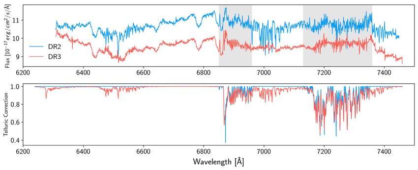
12 S. M. Croom et al.

Figure 10. A comparison of the red arm 3 arcsec aperture spectrum for galaxy 136602 from DR2 (blue) and DR3 (orange). The top panel shows the flux, while
the bottom panel shows the telluric correction function applied to each spectrum. The grey shaded regions indicate the two bands that telluric correction was
applied to in DR2, between 6850 and 6960Å, and between 7130 and 7360Å. Comparatively, in DR3 we allow for telluric correction to the entire red spectrum.
The offset between the DR2 and DR3 fluxes is due to differences in the flux calibration.

lent to distance along the slit) and wavelength. We compare the new (PCA) in the reduced wavelength calibrated and sky–subtracted
sky subtraction residuals (Figs. 8b and d) to those from DR2 [Figs. data that makes use of the algorithm built into 2dfDR (Sharp &
8a and c; see also Fig. 3 of Scott et al. (2018)]. In both the blue Parkinson 2010).
and red arms of AAOmega the systematic sky residuals are lower in In the first stage of the PCA correction we generate principal
the DR3 reductions. For example, the increased residuals near the components of the 5577 Å line residual in a narrow 6Å window
edge of the CCD seen in DR2 data are substantially reduced. The around the line. A smooth (median filtered) continuum is subtracted
systematic residuals below 4000Å ˙ are also reduced, largely because from the spectra and then the faintest 10 per cent of fibres (which
of the revised sky combination. will be dominated by sky emission) are used to generate principal
 A weak residual gradient from top to bottom of the CCD components. Only the first three principal components are used at
remains in the sky subtraction. This is at the level of ' ±0.5 percent. this point. Weights for each component are calculated to minimize
We suspect that this is caused by a small ( 0.1 pixels from top the sky line residual in the core of the line. The aim of this first stage
to bottom) relative stretch of the fibre locations as the slit moves is to minimize the residual in the core of the line so that it does not
through the night. We previously noted (Sharp et al. 2015) that dominate the PCA in the next stage.
due to the boiling off of liquid nitrogen the AAOmega cameras The second stage of the PCA correction generates components
systematically shift through the night by ∼ 0.03 pixels per hour. over a 100 Å window centred on the 5577Å line. Again only the 10
To account for this we apply a shift between the fibre ‘tramlines’ percent faintest fibres are used to generate the principal components.
measured on a flat field and those observed in the on–sky data. In this second stage the first ten principal components are used to
However, for each 0.1 pixel shift, the optics of the spectrograph minimize the sky residuals. Once the model is generated for the sky
also cause a relative ' 0.03 pixel stretch in the fibre locations residuals it is smoothed using a median filter in the fibre direction (of
from top to bottom of the CCD. This small misalignment leads to width 101 fibres). This is because in a small number of cases very
slightly different fluxes extracted. Future updates to 2dfDR should bright galaxies can have real small-scale structure in their spectra
incorporate a correction for this effect. removed by the PCA. However, the scattered light residual around
 To further quantify our sky subtraction accuracy we estimate the 5577 Å line varies slowly across the slit. The median filtering
the median fractional continuum residual in each sky fibre (this maintains excellent correction of scattered light, and removes any
minimizes the impact of shot-noise on the measurement). We then negative impact on bright galaxies. An example is shown in Fig. 9
calculate the median of the absolute value of all these residuals for object 289198 that compares SAMI 3 arcsec diameter aperture
across all sky fibres in the entire SAMI DR3 data set. In the blue spectra from DR2 and DR3, as well as an SDSS spectrum of the
arm we find a median continuum sky residual of 0.76 percent (and same object. The DR2 data shows a significant residual around
a 90th percentile of 2.9 percent), compared to the DR2 value of 1.2 the 5577 Å line (cyan line) that is completely removed in DR3
percent (90th percentile of 4.6 percent). In the red arm the median (blue line). It is also worth noting that the overall shape of the
continuum sky residual is 0.72 percent (90th percentile 2.8 percent) spectrum from DR3 more closely matches the SDSS spectrum due
compared to 0.90 percent (90th percentile of 3.1 percent) in DR2. to improvements in flux calibration that will be detailed below.
 A third improvement focused on the 5577 Å night sky line. As
discussed in Section 3.1, contamination in the dewar of the blue arm
 3.4 Telluric Correction
of AAOmega causes enhanced scattered light. The scattered light
modelling approach described in Section 3.1 reduced the residual The handling of telluric correction has changed substantially since
scattered light, typically by a factor of 2 or more. However, for the previous data releases, going from a comparatively straightforward
more severely affected frames a significant residual was still visible. polynomial interpolation approach, to using the dedicated telluric
To remove this we applied a two-stage principal component analysis feature-fitting software molecfit (Smette et al. 2015; Kausch et al.

 MNRAS 000, 1–27 (2021)