The Seismo-Performer: A Novel Machine Learning Approach for General and Efficient Seismic Phase Recognition from Local Earthquakes in Real Time

Article

The Seismo-Performer: A Novel Machine Learning Approach
for General and Efficient Seismic Phase Recognition from
Local Earthquakes in Real Time
Andrey Stepnov 1,*, Vladimir Chernykh 2, and Alexey Konovalov 1

 1 Far East Geological Institute, Far Eastern Branch, Russian Academy of Sciences, 690022 Vladivostok, Russia;
 director@fegi.ru
 2 Khabarovsk Federal Research Center, Far Eastern Branch, Russian Academy of Sciences, 680000 Khaba-

 rovsk, Russia; admvc@ccfebras.ru
 * Correspondence: a.stepnov@geophystech.ru; Tel.: +7-914-757-66-27

 Abstract: When recording seismic ground motion in multiple sites using independent recording
 stations one needs to recognize the presence of the same parts of seismic waves arriving at these
 stations. This problem is known in seismology as seismic phase picking. It is challenging to auto-
 mate the accurate picking of seismic phases to the level of human capabilities. By solving this prob-
 lem, it would be possible to automate routine processing in real time on any local network. A new
 machine learning approach was developed to classify seismic phases from local earthquakes. The
 resulting model is based on spectrograms and utilizes the transformer architecture with a self-at-
Citation: Stepnov, A.; Chernykh, V.; tention mechanism and without any convolution blocks. The model is general for various local net-
Konovalov, A. The Seismo- works and has only 57 k learning parameters. To assess the generalization property, two new da-
Performer: A Novel Machine tasets were developed, containing local earthquake data collected from two different regions using
Learning Approach for General and a wide variety of seismic instruments. The data were not involved in the training process for any
Efficient Seismic Phase Recognition model to estimate the generalization property. The new model exhibits the best classification and
from Local Earthquakes in Real computation performance results on its pre-trained weights compared with baseline models from
Time. Sensors 2021, 21, 6290.
 related work. The model code is available online and is ready for day-to-day real-time processing
https://doi.org/10.3390/s21186290
 on conventional seismic equipment without graphics processing units.

Academic Editor: Nunzio Cennamo
 Keywords: seismogram; spectrogram; transformer; attention; CNN; deep learning; seismic phase;
 real-time automation; classification; computational efficiency; local seismic network
Received: 21 August 2021
Accepted: 16 September 2021
Published: 19 September 2021

Publisher’s Note: MDPI stays neu- 1. Introduction
tral with regard to jurisdictional Phase picking is a routine task in the processing of local seismological monitoring
claims in published maps and institu- data. The complete automation of this task has become increasingly important, especially
tional affiliations.
 in connection with the growth of seismic networks with inexpensive instruments and the
 increase in the number of Internet of Things (IoT) devices [1,2].
 Phase picking automation is a challenging problem. The number of lower magnitude
 earthquakes has grown exponentially [3]; however, the amplitudes of many earthquake
Copyright: © 2021 by the authors. Li-
 signals are weakened to the level of seismic noise or less with decreasing earthquake mag-
censee MDPI, Basel, Switzerland.
 nitudes. Improving the completeness of the earthquake magnitude catalog is a central
This article is an open access article
distributed under the terms and con-
 goal of local seismological monitoring since a comprehensive catalog provides more in-
ditions of the Creative Commons At-
 formation about the seismic regime.
tribution (CC BY) license (http://crea- Another issue is the configuration of the seismic network. A wide variety of sensor
tivecommons.org/licenses/by/4.0/). types, site soil conditions, and levels of seismic noise can exist inside a single network. Of
 course, this can differ from one network to the next. Consequently, the registered shape
 of a seismic signal can vary significantly, and a general algorithm is needed to address the

Sensors 2021, 21, 6290. https://doi.org/10.3390/s21186290 www.mdpi.com/journal/sensors

Sensors 2021, 21, 6290 2 of 11

 phase picking task in a manner meeting or exceeding human effort for data coming from
 any local seismic network.
 Machine learning techniques allow us to fit the parameters of an arbitrary function
 utilizing existing labeled data to make accurate predictions on new data coming from the
 same complex distribution. Usually, phase picking automation is treated as a classification
 task. One approach is to use split wave data on small windows (4–6 s) that contain only
 one centered pick or noise, e.g., in [4,5]. Each window or sample is considered to belong
 to one of three classes. The processing of small windows of waveform data is more suita-
 ble for real-time seismic systems because ground motion data are received continuously
 in small chunks. Thus, each successive chunk can be added to the previous contiguous
 data to form the length of the window and be fed directly into the fitted model for class
 detection. Since the window length is small, detecting the arrival of P/S times from earth-
 quakes occurs within a few seconds after the arrival of the data with the registered phase.
 However, the exact detection time can slightly vary depending on the implementation of
 a sliding window algorithm. For this approach, in most machine learning architectures,
 convolutional neural networks (CNNs) have the lowest error rates in terms of signal-to-
 noise discrimination [5]. Moreover, CNN-based models such as the generalized seismic
 phase detection model (GPD) demonstrate efficiency for classifying local seismic phases
 at the human performance level [4].
 Another approach is to process earthquake length windows (30–60 s) with more com-
 plex triggers, e.g., [6,7]. The output of this type of model is a probability distribution over
 the window length. For example, PhaseNet [7] outputs P/S phases and noise distributions,
 while the earthquake transformer model (EQT) [6] provides P/S phases and earthquake
 detection triggers. These models have good accuracy when scanning archives, but this
 approach is not suitable for real-time processing due to the required long input window
 length. However, this approach leads to complex models that are difficult to optimize in
 terms of computational efficiency.
 However, the generalization properties of machine learning models have not been
 well tested or assessed [8]. Intuitively, the shape of seismic signals from local earthquakes
 must be preserved from one network to another, even if they are affected by noise and
 other factors. In this work, we aimed to create a model for accurately picking P and S
 waves from local earthquakes in real time. To test the generalization property, we intro-
 duced two datasets that contain P and S waves recorded from local earthquakes in differ-
 ent regions of the earth. That data were not involved in the training process for any model
 to estimate the generalization property. The models presented in the work have the best
 indicators of the accuracy of the TOP-1 classification of seismic phases from local earth-
 quakes for test datasets.
 Typically, seismic data servers are not equipped with graphics cards or any special
 hardware. We developed the most efficient model, suitable for use on the central pro-
 cessing unit (CPU) during inference. On GitHub, we provided the model implementation,
 code examples, helpful tools for scanning seismic archives, and pretrained most suitable
 weights. In this way, it is possible to implement a phase recognition unit in real-time seis-
 mic data processing systems, such as earthquake early warning systems, and in many
 seismological centers that process data, to quickly inform about recent earthquakes and
 their impacts.

 2. Materials and Methods
 Recent advances in solving natural language processing problems applied to image
 classification tasks have shown that transformer architecture with an attention mechanism
 [9] can outperform state-of-the-art CNN-based models [10]. Moreover, the transformer
 architecture lacks some of the inductive bias inherent in CNNs [10]; therefore, the trans-
 former architecture is more generalized. To test the performance of the transformer archi-
 tecture, we developed a new model for phase classification of local earthquakes.

Sensors 2021, 21, 6290 3 of 11

 An overview of the model design is shown in Figure 1. We followed the original
 image recognition model based on transformer architecture [10], with modifications spe-
 cific to the seismic data. The input sample is 4 s 3-channel 100 Hz waveform data recorded
 by a local velocity seismograph. A raw signal from a digitizer was normalized by the ab-
 solute maximum amplitude observed on any of the three components. All the data were
 detrended and high-pass filtered above 2 Hz. We removed the original date and time
 stamps, so each entry started at 0 and had 400 samples in total.

 Figure 1. Seismo-performer model overview.

 First, the spectrogram was computed as a 2D representation of the raw signal for each
 channel. To this end, we successively applied the short-term Fourier transform (STFT),
 calculated the magnitude to obtain the floating-point tensor after a complex STFT opera-
 tion, and finally, converted the magnitudes to decibels. Then, we normalized the data us-
 ing the maximum absolute scaler, as this leads to more stable training results. During the
 STFT operation, seismology-specific parameters were applied (Table 1) to obtain an ade-
 quate spectrogram that represents the seismic phases more clearly than the raw signal.

 Table 1. The Seismo-Performer model configuration parameters.

 Parameter Value
 Number of FFTs 64
 Hop length 16
 Spectrogram dims (H, W, C) 22 × 33 × 3
 Patch size 1 (P1) 22
 Patch size 2 (P2) 3
 Number of patches (N) 11
 Projection dim (D) 48

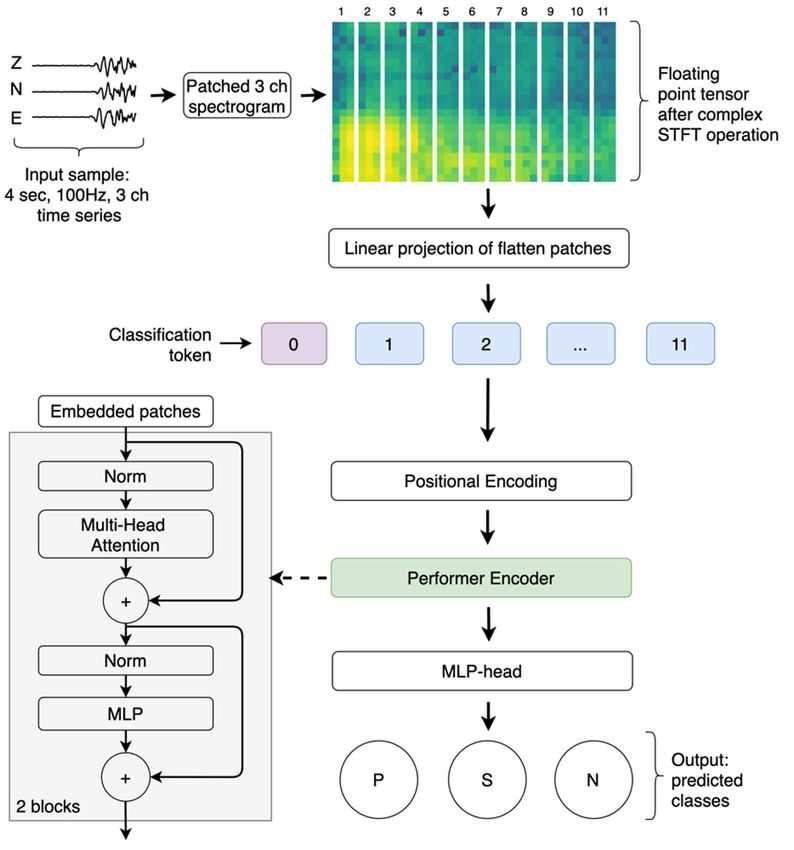
Sensors 2021, 21, 6290 4 of 11

 Performer layers (L) 2
 MLP hidden layer size 96
 MLP output layer size 48
 Number of attention heads 2
 Dropout rate 0.1
 Total trainable parameters 57, 123

 Next, we handled the spectrogram as an image similar to the vision transformer ap-
 proach [10]. The two-dimensional (2D) spectrogram = ℝ × × was reshaped into a se-
 quence of flattened 2D patches = ℝ ×( ∙ ∙ ) , where H and indicate the resolution
 of the original spectrogram, is the number of channels, 1 and 2 are the patch sizes
 along the H and dimensions, and = ( ∙ )/( 1 ∙ 2) is the resulting number of
 patches. We applied rectangular patches to the spectrogram, which differs from the
 squared regions in the original vision transformation approach, as they lead to a more
 accurate classification in our specific model.
 Subsequently, we mapped the patches to dimensions with a trainable linear pro-
 jection to obtain embedded data with a fixed latent vector size as follows:
 ×( ∙ ∙ ) ×
 : ℝ ⟶ℝ (1)
 Next, we added a learnable classification token and position information to the em-
 bedded patches as follows:
 = , , ,…, + , ∈ ℝ( )×
 (2)
 where is the classification token, is the positional information, and is the
 resulting sequence that contains embedded patches with positional encoding.
 The core block of the proposed model is the transformer encoder [9], which consists
 of layers following one another in a sequential manner,
 = MSE(LN( )+ ), = 1, … , (3)
 = MLP(LN( ) + ), = 1, … , (4)
 where LN is the layer normalization function, MSE is the multiple head attention, and
 MLP is the simple feed-forward neural network with GELU [11] nonlinearity. To improve
 computational efficiency, we replaced the original multiple head attention operation
 (MSA) with the FAVOR+ mechanism (MSE) [12], which has linear space and time com-
 plexity to form performer layers at the end.
 Finally, we used the representation state of the classification token that passed
 throughout the performer encoder to perform the classification step as follows:
 ℙ( , , ) = SoftMax(MLP– head( )) (5)
 where is the representation state of the classification token given from the performer
 encoder output, and MLP– head is the feed-forward neural network with one hidden
 layer, which has the same configuration to MLP inside performer layers. To treat the out-
 puts of the model as class probabilities, we applied the SoftMax activation function.
 To configure the resulting model, we selected a rectangular patch size of 1 × 2 =
 22 × 3, with projection dimensions of = 48, and = 2 consecutive layers inside the
 performer encoder. The MSE and MLP functions have their own parameters, such as the
 number of attention heads and dense units. We set 2 heads for MSE. For the MLP and
 MLP– head hidden layers, we picked an equal density of 96 units. The final Seismo-Per-
 former configuration has 57, 123 trainable parameters (Table 1). To prevent overfitting,
 we added dropout layers with a constant rate (0.1) between the dense layers. In addition,
 a relatively small projection dimension ( ) is also an overfitting prevention mechanism.

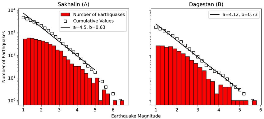
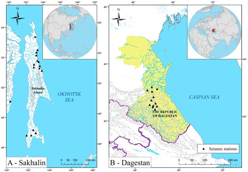
Sensors 2021, 21, 6290 5 of 11

 The implementation of the model and its configuration, the pretrained best-fitted
 weights, the code examples, and documentation are available online (see Data Availability
 Statement).
 To train and validate the model, we used 4.5 million 3-component 4 s seismograms
 recorded in Southern California [13], as this is the largest available dataset of local earth-
 quakes. To additionally test the model, we used local earthquake data collected from two
 different regions using a wide variety of seismic instruments. These data were not in-
 volved in the training process so as to estimate the generalization property as accurately
 as possible.
 The first region was Sakhalin Island (Figure 2A). This region’s local seismic network
 extends along Sakhalin and is notably sparse. On average, earthquakes here are localized
 at only 3 stations. Seismic stations are installed near settlements due to the need for a
 central power supply and the availability of mobile network coverage. In general, these
 are noisy stations. This seismic network was originally established to monitor seismic in-
 duction in connection with oil and gas production in the northern Sakhalin region. The
 seismic network is mainly composed of short-period sensors, such as Lennartz LE3D-Lite
 and OSOP Raspberry Shake. We selected earthquakes that occurred between September
 2006 and March 2021 and filtered out weak events below M1.0 or source depths ≥ 50 km.
 In total, the dataset for Sakhalin after filtration contained 4702 local earthquakes (Figure
 3A).

 Figure 2. Location of local seismic networks and the geometry of the stations for Sakhalin (A) and
 Dagestan (B) regions that were used for the data acquisition.

Sensors 2021, 21, 6290 6 of 11

 Figure 3. The cumulative Gutenberg–Richter frequency-magnitude distribution of seismic events
 across Sakhalin (A) and Dagestan (B) datasets, lines are the best fitting values.

 The second region was located in the northern Caucasus in the center of Dagestan
 (Figure 2B). This seismic network was created to monitor the seismic regime in the vicinity
 of hydroelectric power plants. Each seismic station is equipped with a Guralp CMG-6T
 broadband sensor. On average, earthquakes are localized by 6 or more stations. We used
 data from January 2018 to June 2019 and the same filters used for Sakhalin to obtain 1750
 events in total (Figure 3B).
 To construct both datasets, we selected only those manually picked phases that were
 recorded by a station with an epicentral distance of less than 300 km to track only local
 events. For impulsive seismic noise sampling, a short-term average/long-term average
 (STA/LTA) filter was applied to continuous data with a trigger factor equal to 3.5. We also
 verified that the noise was not actually a seismic event. There was insufficient impulse
 noise for the Dagestan dataset. To prevent class imbalance, we collected more noise sam-
 ples by picking wave windows starting 5 s before randomly choosing the P-wave pick.
 The summary information about datasets is shown in Table 2. The Sakhalin and Dagestan
 datasets presented in this work are available online in HD5 format (see Data Availability
 Statement).

 Table 2. Summary of local earthquake datasets. Each sample is 4 s long at 100 Hz (400 points in
 total). The data were high-pass filtered above 2 Hz, and a trend was removed.

 Dataset Samples Per Class Total Samples Data Time Range Reference
 Sakhalin 3.3 k 9.8 k 2006–2021 This work
 Dagestan 9.4 k 28.1 k 2018–2019 This work
 California 1.5 m 4.5 m 2000–2017 [13]

 3. Results
 To report the results, we trained the Seismo-Performer model several times. First, we
 randomly split the seismograms from the California dataset (Table 2) into training (80%)
 and validation (20%) sets. Then, the model was compiled with a cross-entropy loss func-
 tion and the ADAM optimization algorithm [14]. The model was trained using mini-
 batches of 480 records and a learning rate of 0.001 on the NVIDIA Tesla P100-SXM2 graph-
 ical processing unit for approximately 3.8 h. The training process was terminated after 48
 epochs (full iterations through the training dataset) on average since there were no per-
 formance increases in the validation data for the last five epochs. After completing the
 training, we evaluated the fitted model on the Sakhalin and Dagestan test datasets and
 recorded the results. Then, we randomly partitioned the California dataset again with a
 different random state, compiled, fit the model, and reported the results using the same
 procedure as in the first step. The training process was completely stopped after 10

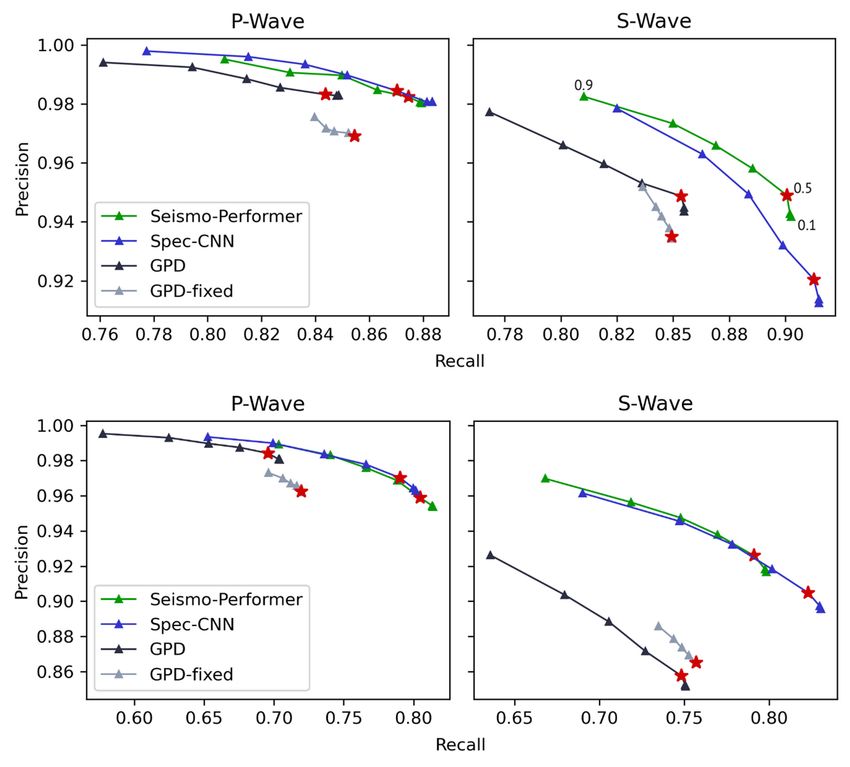
Sensors 2021, 21, 6290 7 of 11

 split/train iterations due to the absence of significant variability in the indicators during
 the validation and testing of the data.
 To further evaluate the generalization of the model, we performed the above training
 procedure on a specific Sakhalin dataset and tested on all the data from California and
 Dagestan. The training, testing, and validation code is available online as a Google Colab
 notebook (see Data Availability Statement). We fixed random seeds to provide nearly the
 same reproducible results, however, they may differ slightly due to the stochastic nature
 of machine learning algorithms.
 To compare the accuracy metrics of the Seismo-Performer model, we applied three
 suitable models using the same input sample. First, we replaced the Performer block with
 CNN after the spectrogram to build the Spec-CNN model. The accuracy metrics of the
 spectrogram-based models were compared with the original CNN-based GPD model,
 which is the state-of-the-art model for short window length raw seismic signal processing.
 Since the code of the GPD model has not been updated for 3 years [15], we redeployed
 this architecture in the latest version of the machine learning framework to speed up the
 learning and inference times. We designated the reconstructed GPD model as a fixed
 GPD. All these models were fitted using the same procedure as for the Seismo-Performer
 model.
 To assess the accuracy of the models, the TOP-1 score was used. That measure checks
 if the top class with the highest SoftMax value matches the true label. The TOP-1 valida-
 tion and test data accuracy for all the tested models are shown in Table 3. It can clearly be
 seen that the spectrogram-based models outperformed the GPDs across all validation and
 testing datasets. The difference in the accuracy of the validation data is less noticeable
 because it comes from the same dataset as the training data for all models. The distinction
 of the TOP-1 metric is clearer for the test datasets, which may indicate better generaliza-
 bility of the Seismo-Performer and Spec-CNN models. This is notable, although when
 training on the Sakhalin dataset of only 7.84 k samples, the difference in accuracy rates for
 the test data was much higher (Table 3, Panel B). Spectrogram models better learn the
 shape of waveforms of local earthquakes even with small amounts of data and, therefore,
 tend to be more general. To examine the differences in accuracy, we plotted the preci-
 sion/recall curves of the test datasets for all the models with various prediction thresholds
 (Figure 4). Metrics are defined as follows:

 = , (6)

 where is a true positive P-phase that is marked correct by the model and matches a
 human label. is a false-positive P phase, classified as P, but in reality it is an S phase.
 Additionally, is a false-positive P phase classified as P, but it is actually noise class.

 = , (7)

 where is a false-negative P phase, which is designated by the model as S, but it is
 P. Additionally, is a false-negative P phase, which marked a true P as some noise.

 Table 3. Comparison of the TOP-1 accuracy in percent (±std.dev.) and inference times on CPU1 in seconds on test datasets.
 All models were fitted 10 times on the California (Panel A) and Sakhalin (Panel B) train sets with different random seeds.
 We reserved 20% of the training dataset for validation at each iteration with different seeds.

 Train Data (Frac.) Test Data (Frac.) Seismo-Performer Spec-CNN GPD-Fixed GPD [4]
 Sakhalin (1.0) 90.69 ± 0.2 91.43 ± 0.2 89.21 ± 0.5 89.08 ± 0.9
 Panel A
 Dagestan (1.0) 84.57 ± 0.7 85.32 ± 0.4 81.94 ± 0.9 81.11 ± 1.2
 California (0.8)
 California (0.2) 2 98.71 ± 0.01 98.80 ± 0.03 98.63 ± 0.02 98.64 ± 0.06
 Sakhalin (0.2) 2 93.71 ± 0.4 95.18 ± 0.6 92.40 ± 1.1 93.37 ± 0.4
 Panel B
 Dagestan (1.0) 83.63 ± 0.7 86.43 ± 0.5 73.03 ± 0.6 73.65 ± 0.5
 Sakhalin (0.8)
 California (1.0) 85.59 ± 2.1 85.05 ± 0.8 81.09 ± 1.0 82.31 ± 0.9
 Parameters 57 k 176 k 1742 k 1742 k

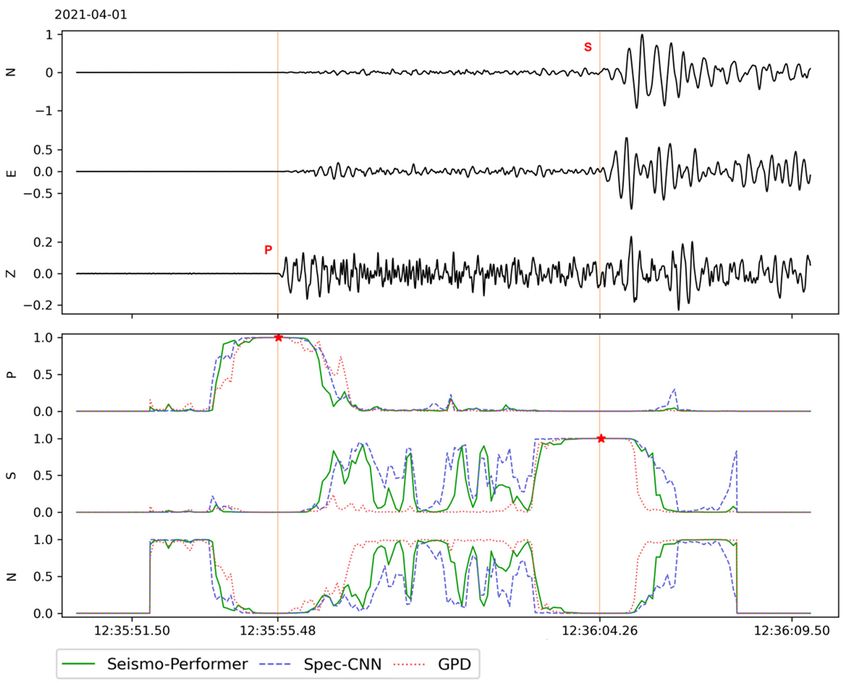
Sensors 2021, 21, 6290 8 of 11

 CPU1 inference time (sec) during 24 h 3 ch ar-
 56.2 ± 0.3 82.8 ± 0.3 89.7 ± 0.5 123.6 ± 0.4
 chive scan with 40 ms shift
 1 Intel(R) Xeon(R) CPU E3-1270 under Linux Kernel-based Virtual Machine (KVM) with 2 virtual cores. 2 20% of the dataset

 was used for validation during training.

 (a)

 (b)

 Figure 4. Precision/recall curves for the Seismo-Performer, Spec-CNN, and GPD classifiers on the Sakhalin (a) and Dage-
 stan (b) datasets. The models were trained on the Southern California dataset only. Precision and recall were computed
 for different probability thresholds from 0.1 and 0.9 in increments of 0.1, resulting in nine precision and recall values for
 each classifier/dataset. Red stars show values for a probability threshold of 0.5.

 The precision/recall metrics for S phase were defined in the same fashion.
 We can conclude that for all cases, the Seismo-Performer and Spec-CNN had signifi-
 cantly better recall rates with about the same precision, compared with the GPD. This is a
 significant finding that is detailed in Section 4.
 To assess computational efficiency, we developed a miniSEED [16] archive scanner.
 This tool processes 24 h, single-channel archive files, similar to those generated by the
 BUD schema [17], which is a common way of storing continuous data from local instru-
 ments. The scanner itself has many configuration options, explained in detail in the
 GitHub documentation (see Data Availability Statement). The most critical option is off-
 setting (shift) the 4 s sliding window. We chose 40 ms as the default and we explain our
 reasoning in Section 4. An example of archive scanning using different models is shown
 in Figure 5. With this tool, we measured the models’ inference times on a 24 h 3 ch archive

Sensors 2021, 21, 6290 9 of 11

 with a sliding window shift of 40 ms, using only the central processor unit (Table 3). The
 Seismo-Performer model was more than twice as fast as the original GPD, and nearly 40%
 as fast as the fixed GPD. The Seismo-Performer model is the fastest model with almost the
 same accuracy compared with the Spec-CNN and, therefore, is the most suitable for day-
 to-day processing.

 Figure 5. An example of the model’s prediction during the processing of a 1 min seismogram. This
 is the NYSH seismic station with a 3-channel component “ENZ” (East, North, Vertical) located 97
 km from the epicenter of an M3.1 local earthquake on northern Sakhalin [18]. “P”, “S” and “N”
 indicate the probability (SoftMax values) of predicting P/S phases and noise, respectively. The red
 vertical lines are the manually picked P and S arrival times. The pentagrams show the maximum
 SoftMax values for predicting the seismic phase class, which are nearly the same for each model.

 4. Discussion
 For the short window length approach, each 4 s sample is considered to belong to
 exactly one class. The main objective of this study was to accurately pick the arrival times
 of seismic phases to utilize this information for further routine processing. To this end, we
 implemented a sliding window method, and the 4 s window was shifted to smaller times,
 in milliseconds, to form a series of overlapping 4 s samples. The sample with the maxi-
 mum SoftMax probability for a particular class, exceeding the configured threshold pa-
 rameter, is selected by the sliding window algorithm as the sample containing the seismic
 phase (P or S). The final arrival time of a seismic phase is picked by a central point of the
 selected sample since all picks were centered in the training set. All the models considered
 in this study accurately pick an arrival time. The accuracy of the picking time is affected
 only by the window shift parameter. For example, if we set a 10 ms shift, we can center
 pick more precisely and, hence, can obtain more accurate pick times considerably close to
 those of human ability. On the other hand, a very small shift results in more counts; for a
 value of 10 ms, we obtain 858,349 4 s windows in a 24 h seismogram case to feed to a
 model, which affects the inference time. However, there is some inaccuracy in the predic-

Sensors 2021, 21, 6290 10 of 11

 tions of a fitted model, uncertainty in human labeling, time synchronization errors (espe-
 cially in the case of the Network Time Protocol), etc. Finally, we chose 40 ms as the default
 optimal shift value (which led to a 4-fold decrease in the number of samples), which does
 not significantly affect the errors in the localization of an earthquake source.
 False positives are problems that occur when testing models with continuous data,
 especially in noisy stations. This is not a special case for the models proposed in this study
 and affects all existing models, including PhaseNet and EQT. This issue can be corrected
 by using the prediction threshold parameter. However, false positives should be distin-
 guishable in terms of SoftMax probabilities and have lower values, compared with true
 seismic phases. In this case, we can set the prediction threshold high enough to filter out
 false positives. This is the reason the better recall rate (Figure 4) is so important. After
 extensive testing of our models on continuous data, we chose 0.9997 and 0.9995 as the
 default prediction thresholds for the P and S phases, respectively.
 In regard to EQT, another state-of-the-art model using the long window approach,
 since the framework propagates different methods of prediction, we resliced the Sakhalin
 and Dagestan samples as follows: The records of the earthquakes were sliced to 1 min
 lengths, totaling 2576 and 6898 samples from the Sakhalin and Dagestan continuous data.
 To evaluate false positives more precisely, we added the same proportion of samples with
 impulse noise picks and normal seismic noise from each source of the data. We flagged
 true positives if the model predicted a phase within ±2 s of the true label and false positives
 otherwise. The model accuracy was only evaluated on the P and S labels without noise
 class. We used pretrained weights and the default settings of the EQT framework. Even-
 tually, we achieved 67.97% and 46.02% accuracy for the Sakhalin and Dagestan test sets,
 respectively. These results are less general (Table 3, Panel A). However, EQT is a very
 powerful tool, especially it has very low false-positive rates on seismic noise records (less
 than 0.01%). Better results can be achieved by training this model on local earthquake data
 only, such as Southern California data [13], and optimizing the prediction hyperparame-
 ters (normalization, filtering, thresholds, etc.)

 5. Summary and Conclusions
 The new machine learning models were developed for accurately picking seismic
 phases from local earthquakes on the level of human capabilities. The models process the
 signal based on a spectrogram rather than raw waveforms. This method made it possible
 to reduce the number of trained parameters and build more general models for recogniz-
 ing seismic arrivals. Using two new test datasets, the best P/S phase prediction accuracy
 for the new technique is fully demonstrated. The Seismo-Performer is one of the proposed
 spectrogram-based models that demonstrates the best computational efficiency through
 the use of the attention mechanism.
 Since the models process 4 s input samples, they are suitable for real-time continuous
 seismic data processing. The issue of false positives that occur when processing continu-
 ous data can be completely solved by tuning the hyperparameters. With the supplied
 models code, pretrained weights, and supporting tools, machine learning processing can
 be quickly deployed to existing seismic data centers. In the case of Seismo-Performer, only
 the CPU can be used without any expensive acceleration hardware.

 Author Contributions: Conceptualization, A.S. and V.C.; data curation, A.S.; formal analysis, A.S.;
 funding acquisition, A.K.; investigation, A.S.; methodology, A.S.; project administration, A.S.; re-
 sources, A.S.; software, V.C.; supervision, A.S.; validation, A.S., V.C. and A.K.; visualization, V.C.;
 writing—original draft preparation, A.S.; writing—review and editing, A.K. All authors have read
 and agreed to the published version of the manuscript.
 Funding: This research received no external funding.
 Institutional Review Board Statement: Not applicable.
 Informed Consent Statement: Not applicable.

Sensors 2021, 21, 6290 11 of 11

 Data Availability Statement: The implementation of the model and its configuration, the pretrained
 best-fitted weights, the code examples, and useful tools for continuous archive scanning and docu-
 mentation are available online at GitHub: https://github.com/jamm1985/seismo-performer (ac-
 cessed on 18 September 2021). Datasets for Sakhalin and Dagestan are available online in HD5 for-
 mat at Google Drive (the links are also present on the GitHub page):
 https://drive.google.com/file/d/1dH2JF9TQmyB6GpIB_dY1jiWAI5uqp6ED (accessed on 18 Septem-
 ber 2021), https://drive.google.com/file/d/156w3I9QVnhkCo0u7wjh-c6xekE9f6B3G (accessed on 18
 September 2021).
 Acknowledgments: The authors are grateful to GEOPHYSTECH LLC for providing data from the
 local seismic networks of Sakhalin and Dagestan, which made this study possible. The studies were
 carried out using the resources of the Center for Shared Use of Scientific Equipment “Center for
 Processing and Storage of Scientific Data of the Far Eastern Branch of the Russian Academy of Sci-
 ences” [19] funded by the Russian Federation represented by the Ministry of Science and Higher
 Education of the Russian Federation under project No. 075-15-2021-663.
 Conflicts of Interest: The authors declare no conflict of interest.

References
1. Anthony, R.E.; Ringler, A.T.; Wilson, D.C.; Wolin, E. Do Low-Cost Seismographs Perform Well Enough for Your Network? An
 Overview of Laboratory Tests and Field Observations of the OSOP Raspberry Shake 4D. Seism. Res. Lett. 2018, 90, 219–228,
 doi:10.1785/0220180251.
2. Sepulveda, F.; Pulliam, J. The Internet of Geophysical Things: Raspberry Pi Enhanced REF TEK (RaPiER) System Integration
 and Evaluation. Seism. Res. Lett. 2016, 87, 345–357, doi:10.1785/0220150234.
3. Staudenmaier, N.; Tormann, T.; Edwards, B.; Deichmann, N.; Wiemer, S. Bilinearity in the Gutenberg-Richter Relation Based
 on M L for Magnitudes Above and Below 2, From Systematic Magnitude Assessments in Parkfield (California). Geophys. Res.
 Lett. 2018, 45, 6887–6897, doi:10.1029/2018gl078316.
4. Ross, Z.E.; Meier, M.; Hauksson, E.; Heaton, T.H. Generalized Seismic Phase Detection with Deep Learning. Bull. Seism. Soc.
 Am. 2018, 108, 2894–2901, doi:10.1785/0120180080.
5. Meier, M.; Ross, Z.E.; Ramachandran, A.; Balakrishna, A.; Nair, S.; Kundzicz, P.; Li, Z.; Andrews, J.; Hauksson, E.; Yue, Y.
 Reliable Real-Time Seismic Signal/Noise Discrimination with Machine Learning. J. Geophys. Res. Solid Earth 2019, 124, 788–800,
 doi:10.1029/2018jb016661.
6. Mousavi, S.M.; Ellsworth, W.L.; Zhu, W.; Chuang, L.Y.; Beroza, G.C. Earthquake transformer—An attentive deep-learning
 model for simultaneous earthquake detection and phase picking. Nat. Commun. 2020, 11, 1–12, doi:10.1038/s41467-020-17591-w.
7. Zhu, W.; Beroza, G.C. PhaseNet: A Deep-Neural-Network-Based Seismic Arrival Time Picking Method. Geophys. J. Int. 2018,
 216, 261–273, doi:10.1093/gji/ggy423.
8. Lomax, A.; Michelini, A.; Jozinović, D. An Investigation of Rapid Earthquake Characterization Using Single-Station Waveforms
 and a Convolutional Neural Network. Seism. Res. Lett. 2019, 90, 517–529, doi:10.1785/0220180311.
9. Vaswani, A.; Shazeer, N.; Parmar, N.; Uszkoreit, J.; Jones, L.; Gomez, A.N.; Kaiser, L.; Polosukhin, I. Attention Is All You Need.
 arXiv 2017, arXiv:1706.03762.
10. Dosovitskiy, A.; Beyer, L.; Kolesnikov, A.; Weissenborn, D.; Zhai, X.; Unterthiner, T.; Dehghani, M.; Minderer, M.; Heigold, G.;
 Gelly, S.; et al. An Image Is Worth 16 × 16 Words: Transformers for Image Recognition at Scale. arXiv 2020, arXiv:2010.11929.
11. Hendrycks, D.; Gimpel, K. Gaussian Error Linear Units (GELUs). arXiv 2016, arXiv:1606.08415.
12. Choromanski, K.; Likhosherstov, V.; Dohan, D.; Song, X.; Gane, A.; Sarlos, T.; Hawkins, P.; Davis, J.; Mohiuddin, A.; Kaiser, L.;
 et al. Rethinking Attention with Performers. arXiv 2020, arXiv:2009.14794.
13. SCEDC Southern California Earthquake Data Center. Available online: https://scedc.caltech.edu/data/deeplearning.html (ac-
 cessed on 10 August 2021).
14. Kingma, D.P.; Ba, J. Adam: A Method for Stochastic Optimization. arXiv 2014, arXiv:1412.6980.
15. Interseismic/Generalized-Phase-Detection. Available online: https://github.com/interseismic/generalized-phase-detection (ac-
 cessed on 10 August 2021).
16. IRIS: miniSEED. Available online: http://ds.iris.edu/ds/nodes/dmc/data/formats/miniseed/ (accessed on 10 August 2021).
17. IRIS: BUD: Buffer of Uniform Data. Available online: http://ds.iris.edu/ds/nodes/dmc/data/bud/ (accessed on 10 August 2021).
18. M3.1 Earthquake, Sakhalin, Summary. Available online: https://eqalert.ru/#/events/PBzn9vB9 (accessed on 10 August 2021).
19. Sorokin, A.A.; Makogonov, S.V.; Korolev, S. The Information Infrastructure for Collective Scientific Work in the Far East of
 Russia. Sci. Tech. Inf. Process. 2017, 44, 302–304, doi:10.3103/s0147688217040153.