The Spread of COVID-19 and the BCG Vaccine: A Natural Experiment in Reunified Germany - Federal ...
←
→
Page content transcription
If your browser does not render page correctly, please read the page content below
Federal Reserve Bank of New York
                             Staff Reports

      The Spread of COVID-19 and
            the BCG Vaccine:
A Natural Experiment in Reunified Germany

                                 Richard Bluhm
                                Maxim Pinkovskiy

                                 Staff Report No. 926
                                       May 2020

   This paper presents preliminary findings and is being distributed to economists
   and other interested readers solely to stimulate discussion and elicit comments.
   The views expressed in this paper are those of the authors and do not necessarily
   reflect the position of the Federal Reserve Bank of New York or the Federal
   Reserve System. Any errors or omissions are the responsibility of the authors.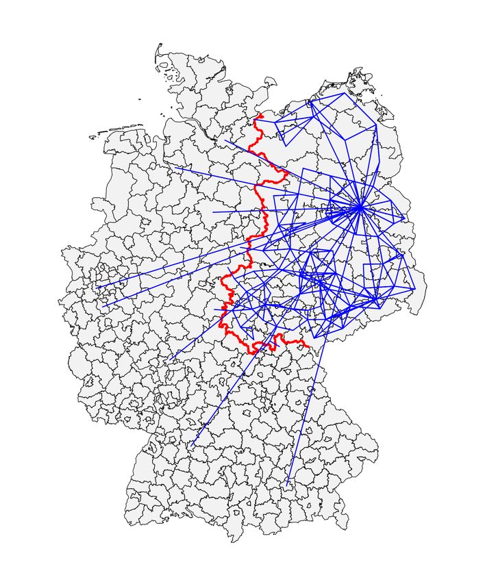
The Spread of COVID-19 and the BCG Vaccine: A Natural Experiment in
Reunified Germany
Richard Bluhm and Maxim Pinkovskiy
Federal Reserve Bank of New York Staff Reports, no. 926
May 2020
JEL classification: C21, I18, J60

                                            Abstract

As COVID-19 has spread across the globe, several observers noticed that countries still
administering an old vaccine against tuberculosis—the BCG vaccine—have had fewer
COVID-19 cases and deaths per capita in the early stages of the outbreak. This paper uses a
geographic regression discontinuity analysis to study whether and how COVID-19 prevalence
changes discontinuously at the old border between West Germany and East Germany. The border
used to separate two countries with very different vaccination policies during the Cold War era.
We provide formal evidence that there is indeed a sizable discontinuity in COVID-19 cases at the
border. However, we also find that the difference in novel coronavirus prevalence is uniform
across age groups and show that this discontinuity disappears when commuter flows and
demographics are accounted for. These findings are not in line with the BCG hypothesis. We then
offer an alternative explanation for the East-West divide. We simulate a canonical SIR model of
the epidemic in each German county, allowing infections to spread along commuting patterns.
We find that in the simulated data, the number of cases also discontinuously declines as one
crosses from west to east over the former border.

Key words: COVID-19, BCG vaccine, SIR model with commuting flows

_________________

Pinkovskiy: Federal Reserve Bank of New York (email: maxim.pinkovskiy@ny.frb.org). Bluhm:
Leibniz University Hannover and University of California San Diego (email: rbluhm@ucsd.edu).
Any errors or omissions are the responsibility of the authors. The views expressed in this paper
are those of the authors and do not necessarily represent the position of the Federal Reserve Bank
of New York or the Federal Reserve System.

To view the authors’ disclosure statements, visit
https://www.newyorkfed.org/research/staff_reports/sr926.html.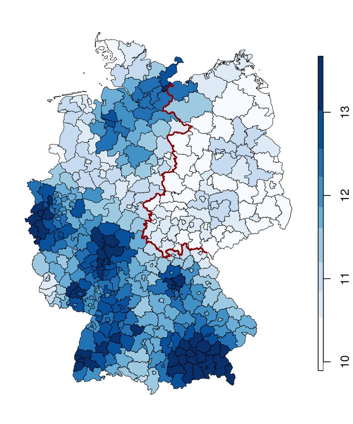
1       Introduction
As COVID-19 has spread across the globe, there is an intense search for treatments and
vaccines, with numerous trials running in multiple countries. In light of this, there is
now a lively controversy over whether the Bacillus Calmette-Guérin (BCG) vaccine against
tuberculosis may somehow protect individuals against COVID-19 or limit its severity.
Multiple studies (see, e.g., Miller et al., 2020, Berg et al., 2020) pointed out that countries
with mandatory BCG vaccination tend to have substantially fewer coronavirus cases and
deaths per capita than countries without mandatory vaccination, and that the intensity of
the epidemic is lower for countries that began vaccinating earlier.1 At least eight clinical
trials are taking place across the globe2 in which some medical workers or volunteers receive
the BCG vaccine to test its effectiveness against COVID-19. These trials are likely to take
at least a year and the virus is still spreading globally at a rapid pace. As of now, the WHO
cautions that there is no evidence that the vaccine protects against the novel coronavirus.3
    In this paper we propose a different way to test the hypothesis that BCG protects a large
share of vaccinated populations against coronavirus: a regression discontinuity analysis of
coronavirus cases at the former border between East Germany and West Germany. This
border separated capitalist West Germany from communist East Germany from 1949 to
1990 until the two countries were reunified as the current Federal Republic of Germany. In
line with many other Western European countries, West Germany discontinued a policy of
de facto universal BCG vaccination (which began in the 1950s) for the general population in
1975, while, equally in line with other former Soviet Bloc countries, East Germany strictly
enforced a policy of mandatory BCG vaccination at birth from 1953 until 1990. Although it is
known that other characteristics change discontinuously at the old East German border (even
before it existed, see Becker et al., 2020, Fuchs-Schündeln and Hassan, 2015, Alesina and
Fuchs-Schündeln, 2007), these differences are considerably smaller than if different countries
or regions are compared. Moreover, areas of Germany on both sides of the discontinuity have
been subject to the same state response to the COVID-19 pandemic. Other discontinuities

    1
      This started a lively debate in the community on the fallacies of cross-country regressions. As our
approach differs from these studies, we only note that other studies which are not based on cross-country
data find no such effects, for example when looking at passengers on the Diamond Princess or when controlling
for countries’ intensity of testing for COVID-19 (Asahara, 2020).
    2
      For example, the BRACE trial in Australia (NCT04327206), the BCG-CORONA trial in the Netherlands
(NCT04328441), and more recent trials in Brazil (NCT04369794), Columbia (NCT04362124), Denmark
(NCT04373291), Egypt (NCT04350931) and the United States (NCT04348370). ClinicalTrials.gov registry
codes are provided in parentheses.
    3
      This warning was based on a review of the available evidence from three cross-country studies.
The scientific briefing is published here (www.who.int/publications-detail/bacille-calmette-gu%C3%
A9rin-(bcg)-vaccination-and-covid-19) and explained further in Curtis et al. (2020).

                                                     1
are also less of a concern since we can exploit variation both in space and across age groups
to improve identification.
    We find a strong discontinuity in cumulative COVID-19 cases across the old East German
border, with cases per million roughly halving at the border as of April 26 2020. This
discontinuity is robust to controlling for other variables that change discontinuously at the
border, such as population density, disposable income, average age and the fraction of the
population over 65, as well as age-adjusted death rates from all causes and from infectious
diseases.4 Importantly, while these control variables are discontinuous at the border, the
discontinuities typically go the “wrong way” in terms of their correlations with characteristics
that usually indicate more vulnerable populations. Counties on the eastern side of the border
are poorer, older and have higher death rates, although they have lower population density,
than counties just to the west of the border. We document that the initial geography of the
outbreak in wealthier and well-connected places implies that these correlations are reversed
from what intuition would suggest. For example, the outbreak is currently stronger in richer,
younger and generally healthier places of Germany.
    Evidence from discontinuities in COVID-19 confirmed cases by age group suggests that
this discontinuity does not come from people on the eastern side of the border being protected
by the BCG vaccine. The timing of the adoption and the cessation of mandatory vaccination
in East and West Germany implies that the only age groups for which discontinuities should
be observed should be individuals between ages 30 and 45, as well as people between ages
59 and 69. For other age groups, there should be no direct effect of the BCG vaccine since
they were either unvaccinated or vaccinated on both sides of the border. However, there is
a discontinuous decrease in COVID-19 confirmed cases of approximately the same size as
one crosses the border into the east for every age group for which we have data, starting
with individuals who are 15 years old (people younger than 15 rarely manifest strong enough
COVID-19 symptoms to get tested).5
    We provide further evidence on what could be giving rise to the discontinuity in
coronavirus cases at the old border to East Germany by considering the matrix of commuter

   4
      Prominent newspapers in Germany have noticed that there is much lower COVID-19 prevalence
in the former East than in the West but offer only suggestive explanations (e.g., Die Zeit,
a     German      weekly,    www.zeit.de/2020/13/coronavirus-ausbreitung-osten-westen-faktoren,
or     Der    Tagesspiegel,    a     Berlin-based     German       daily,   www.tagesspiegel.de/politik/
mehr-flaeche-mehr-alte-warum-der-osten-weniger-unter-corona-leidet/25796940.html).
Moreover, low COVID-19 mortality in Germany as a whole has been the subject of media interest.
    5
      One could expect that vaccinated individuals in a population offer some degree of protection to the
unvaccinated. In fact, medical research (Curtis et al., 2020) suggests that there may be a countervailing
effect as BCG-vaccinated places may have more asymptomatic individuals with a greater propensity to
spread the virus. Even if the overall spillover did offer protection to unvaccinated individuals, the resulting
discontinuity for such individuals should be smaller than for the population affected directly by the vaccine.

                                                      2
flows across German counties. Apart from strong connections between major cities in the
West and Berlin, these flows still generally proceed within the former West or within the
former East rather than between both sides. Since the epidemic started in the West, these
flows imply that it was more likely that it would be transmitted more rapidly and widely
there than in the East. We simulate a SIR model with mobility flows between counties to
asses how mobility patterns shaped the geography of the pre-lockdown outbreak. In line
with our empirical evidence, we find that the model also generates a discontinuity at the
border, with more cases per capita on the western side relative to the eastern side, without
any reference to the BCG hypothesis.
An important caveat is that our study looks only at whether or not there is a long-run
effect of the BCG vaccine (roughly decades after it was administered). The BCG hypothesis
essentially comes in two variants. The broad version suggested by cross-country correlations
hypothesizes that people who have received this vaccine in the past (perhaps with refreshers)
develop no or comparatively milder symptoms of COVID-19 than those who have not, enough
for this to show up in the incidence of novel coronavirus cases around the world. If this were
true, the BCG vaccine would provide a respite to the developing world as the virus spreads
globally, which is why prominent news outlets have reported this correlation.6 This is the
question we address in this paper. However, the BCG vaccine’s positive effect on other viral
infections, such as yellow fever (Arts et al., 2018), is a trained response of the immune system
typically occurring within one to twelve months after it has been administered. The evidence
of such trained responses is mixed (for a review see Kandasamy et al., 2016) although recently
a consensus seems to have emerged that the protective effects on other diseases occur via
epigenetic reprogramming (Kleinnijenhuis et al., 2015, Covián et al., 2019). The narrow
version of the hypothesis suggests that the vaccine might have a short-run effect which could
offer some protection to health workers and other risk groups. Our research design cannot
test this aspect as the vaccine has been discontinued in both parts of Germany for 30 years.
Only the results from randomized trials can answer that question.
The remainder of the paper is organized as follows. Section 2 describes the county-level
data on cases, covariates, and commuter flows. Section 3 discuses the temporal differences
in BCG policies in Germany from partition to reunification and describes our empirical
strategy. Section 4 presents the results for discontinuities in overall cases, the most relevant
covariates, cases by age-groups, and the placebo test with cases simulated from a county-level
SIR model with mobility. Section 5 concludes.
6
See, for example, The New York Times (www.nytimes.com/2020/04/03/health/
coronavirus-bcg-vaccine.html) or Bloomberg News (www.bloomberg.com/news/articles/2020-04-02/
fewer-coronavirus-deaths-seen-in-countries-that-mandate-tb-vaccine).
32 Data
COVID-19 spread in Germany: We obtain counts of cumulative cases of and deaths
from COVID-19 by German county (Kreis) and by age group for every date since February
29 2020 from the Robert Koch Institute’s Coronavirus Dashboard.7 Germany has one of the
most comprehensive testing regimes among the heavily affected countries.8 Nevertheless,
given the difficulties in recording asymptomatic cases of COVID-19 that may still be
contagious, it is very likely that the case counts we employ in this paper are a lower bound
for novel coronavirus infections in Germany.9 Streeck et al. (2020) study a large sample of
the city of Heinsberg—a community with an early a super-spreading event—and estimate
that the true case count is about five times larger than officially registered cases. We proceed
on the necessary assumption that the cumulative reported case count is a valid measure of
COVID-19 intensity in a given subpopulation, and that undercounting errors are uniform
across age groups and locations.
We start our analysis with a map of COVID-19 cases in Germany by county as of April
26 (see Figure 1). The former border between East and West Germany is outlined in red.
The darker the shading of a county, the more novel coronavirus cases per million inhabitants
it has. Several counties with high concentrations stand out (such as Heinsberg, bordering
the Netherlands, and much of Bavaria, both places where the epidemic was first recorded).
It is also clear that there is a greater density of COVID-19 cases around major cities (Berlin,
Hamburg or Stuttgart), similar to the United States. However, we immediately see that
counties just to the west of the former border are a much darker shade of blue than counties
just to its east.
County-level covariates: We collect four groups of county-level characteristics: income
and demographics, historical mortality, and commuting flows. Baseline characteristics of
each county (shapes, names and areas) are from the Federal Agency for Cartography and
Geodesy (Bundesamt für Kartographie und Geodäsi ).
Measures of disposable income in 2017, the age distribution in 2018 (aggregated to
different age groups or shares), and population density in 2018 are taken from official
7
The data are publicly available at corona.rki.de.
8
By April 21 2020, Germany had conducted 2,072,669 tests or about 24,966 tests
per million people (Robert Koch-Institut, 2020). This is almost double the testing rate
in the United States, United Kingdom or South Korea, see www.businessinsider.com/
coronavirus-testing-per-capita-us-italy-south-korea-2020-4.
9
These considerations may make it reasonable to treat cumulative case counts as an indication of the
severity rather than of the incidence of COVID-19, since very mild cases, which may account for the majority
of COVID-19 infections, typically do not lead to testing.
4Figure 1 – Covid-19 cases in Germany, April 26 2020, log(1 + cases/million)
Notes: Illustration of the spatial distribution of COVID-19 cases in Germany as of April 26, 2020. The
map shows the log(1 + cases/million people) in each county using population data from 2018.
statistics published by the federal statistical office and the statistical offices of each state.10
We also collect data on overall mortality (in 2017), mortality from selected infectious
diseases and mortality from respiratory diseases (both in 2016) from the same source.
Germany does not publish age-adjusted mortality figures. Given that the age-profile of
the population varies significantly across counties in Germany, we manually age-adjust all
mortality figures using the corresponding age distribution of the entire country in 2017 or
2016, respectively.11 This allows us to analyze regional mortality differences net of local
demographics.
Last but not least, we use the latest available data on commuting flows published by the
Federal Employment Agency (Bundesagentur für Arbeit). The agency regularly releases
an origin-destination matrix of commuting flows across German counties. These flows
capture about 33 million officially registered jobs (all jobs with social security contributions).
Approximately 39%, or 13 million, of the jobs are in a different county than the primary
10
The data are available at www.regionalstatistik.de/genesis.
11
The age-adjustment re-weights local mortality with the age profile of the entire country. We follow the
direct method used by the U.S. Centers for Disease Control (Klein and Schoenborn, 2001).
5tax residence of the employee. We use the county-to-county data from December 2019
to capture connections between western and eastern counties just before the outbreak of
the novel coronavirus. While this cannot account for all travel flows around the outbreak
perfectly, we assume that such unobserved flows follow the dominant pattern of employees
returning home.12
3 Empirical Strategy
Our study exploits a discontinues change in vaccination policies across the former border
dividing East and West Germany from 1949 until 1990.
Germany had a non-vaccination policy until the end of World War II and did not join
Red Cross-led vaccination campaigns in the early post-war years, even though tuberculosis
was widespread among the war-ravaged population.13 BCG policies then diverged quickly
when the country was divided. In 1953, the German Democratic Republic (GDR)
introduced mandatory vaccination for a variety of diseases, including the BCG vaccine
against tuberculosis.14 The policy lasted until the collapse of the GDR in 1990. The Federal
Republic of Germany only required mandatory vaccination for smallpox from 1949 until the
end of 1975. The BCG vaccine was highly recommended but administered on a voluntary
basis. In practice, vaccination of newborns was near universal by the mid-1960s.15 In 1974,
the policy was changed to vaccinate only children in risk groups and, in 1975, the BCG
vaccine was temporarily withdrawn from the market in the West. Neo-natal vaccination
practically ceased for two years (Genz, 1977). Voluntary vaccination of risk groups continued
thereafter until 1998 (Robert Koch-Institut, 1976, 1998) but few people were vaccinated in
West Germany from 1975 onward or in reunified Germany after 1990. Currently, no BCG
vaccine is licensed in Germany. We summarize these political changes in Table 1. We use
precisely these differences in vaccination policies across the former East and West, as well as
12
A suitable alternative would be an origin-destination matrix derived from mobile phone movements
through the early months of 2020. However, Germany’s strong privacy protection laws have the side-effect
that such products are rarely produced by private companies.
13
This decision was in part due to the “Lübeck vaccination disaster” in which 251 infants were vaccinated
with a BCG vaccine contaminated with live tuberculosis bacteria. Almost all children fell ill with tuberculosis
and 72 died, leading the Interior Ministry to reject BCG vaccination as unsafe in 1930 (Loddenkemper and
Konietzko, 2018).
14
Enforcement in the GDR was strict. “From 1954 on, school children who had not yet been vaccinated
had to present a letter of exemption not only from their parents but also from a physician” (Harsch, 2012,
p. 420). Vaccinations substantially outstripped newborns in the early 1950s, suggesting that young adults
born before the GDR existed where also vaccinated ex post.
15
Due to the decentralized nature of the West German health care system, the initial roll out of the
vaccination policy varied strongly by state in the 1950s. However, by 1964, practically all newborns in West
Germany were BCG vaccinated shortly after birth (Kreuser, 1967).
6across cohorts, to identify the effect of historical BCG vaccination on the spread of COVID-19
cases.
Table 1 – Timeline of vaccination policies in both parts of Germany, 1949 until today
Year West Germany (FRG) East Germany (GDR)
1949 First BCG vaccinations
1951-52 Extended program with GDR
manufactured BCG vaccine
1953 BCG vaccine is licensed Mandatory vaccination (with refresher),
target rate at least 95%
1955 Recommendation to vaccinate all
newborn children
Mid 1960s Near universal vaccination of newborns Near universal vaccination of newborns
1974 Recommendation to only vaccinate
children in risk groups
1975 BCG vaccination temporarily halted
1983 Further restriction to only those children
that have TB in the family
1988 Vaccine recommended only for children
that tested negative for tuberculin and
are risk groups
1990 Reunification, policies of FRG continue Reunification, policies of FRG apply
1998 Vaccination no longer recommended
Notes: Based on Klein (2013) and various sources cited in the text.
We employ two related techniques to exploit these policy discontinuities. For our baseline
estimates, we specify a spatial regression discontinuity (RD) design of the form
yc = α + βEastc + δ1 dc + δ2 (dc × Eastc ) + λs(c) + εc if |dc < b| (1)
where c indexes counties (Kreise), yc is the outcome variable, Eastc indicates whether
the county was part of East Germany before reunification, dc is the distance of county c from
the former East German border (it is negative if Eastc = 0 and positive if Eastc = 1), and
λs(c) is a fixed effect for the border segment associated with county c. Border segments are
defined as pairs of bordering states (Bundesländer ). Note that we drop Berlin throughout the
analysis and focus on the border separating the two larger countries, as Berlin in its entirety
cannot be cleanly assigned to either East or West. Following Gelman and Imbens (2019),
our specification uses an interacted local linear RD polynomial at a variety of plausible
bandwidths b, ranging from 50 km to 200 km. We select this range by computing optimal
bandwidths for the specification without border segment fixed effects according to various
criteria developed in the literature (Imbens and Kalyanaraman, 2011, Calonico et al., 2014).
7They vary by outcome but generally fall somewhere in the range between 80–200 km.
Spatial RD designs identify the causal effect directly at the border if three crucial
assumptions hold (see, e.g., Dell, 2010). First, all other factors besides our treatment variable
(BCG vaccination) should vary smoothly from counties just to the east and just to the west
of the border at the time it was drawn. The strength of the RD approach is that it non-
parametrically controls for these confounders, even if they are unobserved. Second, there
should be no compound treatment, so that counties belonging to the West or East of the
former border vary only according to the BCG regime. Third, there should be no selective
sorting at the border at the time of the treatment. The first and second assumption are
likely to be violated in our setting. As Becker et al. (2020) document, the post-war border is
already visible in many economic variables before World War II and East Germany differed
from West Germany in many more ways than its BCG vaccination policy. Selective sorting
is unlikely during the Cold War years and was probably not motivated by the different BCG
regimes, but selective migration did occur prior to the closing of the border in 1961. Hence,
the simple discontinuity design presented in eq. (1) has a number of flaws.
We address these concerns by additionally exploiting the temporal discontinuity across
cohorts. The RKI data reports COVID-19 cases for several cohorts, including those that
are currently 15–34 or 35–59 years old. Table 1 shows that most members of the first age
group did not get the vaccine anywhere. In the second group, everyone was vaccinated in
the East but only those above 45 years old could have received the vaccine in the West if
they were not part of the small risk group. The effect of pre-World War II confounders does
not vary specifically across these two age groups and any compound treatment mostly affects
the older cohort. We can therefore identify whether BCG vaccinations have an effect on the
COVID-19 cases by simply comparing the regression coefficients across these two groups.
Following Deshpande (2016), we can formalize this comparison by estimating a regression
discontinuity differences-in-differences (RD-DD) specification
yc,a = αa + βEastc + γEastc × Olda + δ1 dc + δ2 dc × Eastc +
(2)
δ3 dc × Olda + δ4 dc × Eastc × Olda + λs(c),a + εc,a if |dc < b|
where a indexes age groups (15–34 and 35–59), Olda is an indicator for the age group 35–
59, and the intercept and the border segment fixed effects are allowed to vary by age group.
The coefficient of interest, γ, delivers an estimate of the difference in discontinuities across
cohorts. The identification assumptions for this specification are less stringent than for the
original RD design because we now allow discontinuities in other controls as long as they are
the same across age groups. In particular, any compound treatment effects are differenced
8out if they are the same at ages 15–34 and 35–59, and selective sorting at the border is
allowed insofar as both age groups are sorting in the same way.
If the BCG hypothesis is true, then we would expect to see a negative discontinuity in
cases for the older cohorts but no discontinuity or a much smaller discrepancy in the younger
cohort. Finding a sizable discontinuity in both cohorts, or no differences in the discontinuity
across cohorts, would be direct evidence against the broad version of the BCG hypothesis
and an indication that something else is driving these results. As our data does not contain
any age group which was recently vaccinated, we cannot assess whether the BCG vaccine
has a short-run effect on those that were vaccinated within the last year.
4 Results
Baseline regression discontinuity results: To formalize the intuition of Figure 1, we
use a regression discontinuity design, in which we nonparametrically estimate coronavirus
prevalence as a function of the distance to the border and compare the estimates just to the
east and just to the west of the border. Our main dependent variable is the logarithm of
unity plus the number of cumulative COVID-19 cases per million in a German county as of
April 26, 2020. As the average German county (Kreis) has about 200,000 inhabitants and
nearly every Kreis has at least one confirmed COVID-19 case, this function behaves very
similarly to the logarithm of cumulative cases per million. Figure 2 presents nonparametric
estimates of the mean of the dependent variable by distance to the border of the former GDR,
with positive distances indicating locations in former East Germany and negative distances
corresponding to locations in former West Germany. We use a bandwidth of 100 km, which
corresponds well to the optimal bandwidth (following Imbens and Kalyanaraman, 2011).
We observe that while the nonparametric estimates are continuous to the left and to the
right of zero, they are very discontinuous at zero with a downward jump of approximately
0.7 log points as one moves from west to east. This implies that there are half as many
cases per capita in a former East German county relative to a West German county just
across the border. This halving of cases dominates the variation in coronavirus prevalence
among counties in the East (where it is uniformly low) and is sizable relative to the average
prevalence in the West. Faraway counties in Bavaria (close to the early outbreaks in Italy)
or near the borders with France and the Benelux countries have the highest cases.
The first row of Table 2 further formalizes our results by estimating eq. (1) for 5 different
bandwidths—50 km, 75 km, 100 km, 150 km and 200 km. The smallest of these bandwidths
entails running the regression on 77 German counties closest to the former border, whereas
the largest of these bandwidths runs the regression on 287 of the 401 counties in Germany.
9Figure 2 – Discontinuity in log(1 + cases/million) at former border
8
7.5
7
6.5
6
5.5
-400 -200 0 200
Distance to the East of Former Border, kilometers
Notes: Illustration of the discontinuity log(1 + cases/million people) across the former border between
West and East Germany. The figure shows non-parametric local polynomial estimates for bins of the
dependent variable, where each bin is 20 km wide. 95% confidence intervals are shaded in grey.
The latter three correspond to the range of the optimal bandwidths discussed in Section 3.16
Different bandwidths alter the variance-bias trade-off in the RD point estimate. The degree
of misspecification error is essentially controlled by the choice of bandwidth. Smaller than
optimal, or undersmoothed, bandwidths create less bias in conventional confidence intervals
than large bandwidths (Calonico et al., 2014), which is why we emphasize the results for 100
km or less. We see that the estimate for a 100 km bandwidth is a drop of -0.83 log points, or
57% of the cumulative COVID-19 case count as one crosses the border from West to East.
This estimate is robust and statistically significant at 99% across bandwidths, ranging from
-0.71 for a bandwidth of 75 km to -0.89 for a bandwidth of 200 km.17
The second row of Table 2 shows that there is also a discontinuity in COVID-19 deaths per
million residents, which is larger in size than the discontinuity in the cumulative COVID-19
cases (although the estimates are noisier and the confidence intervals overlap because deaths
are a small fraction of cases). For a 100 km bandwidth, crossing the border from west to
east entails a 1.05 log point (65% decrease) in the number of deaths per million residents,
with estimates for wider bandwidths showing a 50% larger drop.
16
These bandwidths were computed for specifications without border segment fixed effects, whereas eq. (1)
always includes border segment fixed effects.
17
We present additional robustness of the discontinuity in cumulative COVID-19 cases to alternative
functional forms of the local polynomial in Table B-1 of the Appendix.
10Table 2 – Discontinuities in cases, deaths and other variables
The dependent variable varies by panel
The bandwidth is
50 km 75 km 100 km 150 km 200 km
(1) (2) (3) (4) (5)
Panel A. Log(1+cases/million)
East -.787*** -.710*** -.830*** -.987*** -.890***
(.240) (.149) (.154) (.196) (.143)
Panel B. Log(1+deaths/million)
East -.963** -.860*** -1.05*** -1.48*** -1.59***
(.488) (.308) (.290) (.423) (.201)
Panel C. Disposable income p.c.
East -.084*** -.100*** -.104*** -.128*** -.134***
(.026) (.014) (.005) (.015) (.014)
Panel D. Population density
East -.692** -.584*** -.659*** -.474*** -.102
(.279) (.097) (.230) (.154) (.193)
Panel E. Percent older than 64
East 2.585*** 2.175*** 2.424*** 3.132*** 3.109***
(.889) (.830) (.658) (.616) (.613)
Panel F. Percent older than 45 and younger than 65
East 2.251*** 1.653*** 2.105*** 1.714*** .992**
(.778) (.567) (.546) (.478) (.445)
Panel G. Age-adjusted overall death rate per million
East .057*** .048** .045** .059*** .041*
(.018) (.020) (.020) (.016) (.023)
Panel H. Age-adjusted infectious diseases death rate per million
East 2.048** 1.723* 2.190** 2.630** 2.688**
(.841) (.998) (1.087) (1.146) (1.119)
Panel I. Age-adjusted respiratory diseases death rate per million
East 2.613** 2.191* 2.785** 3.216** 3.310**
(1.109) (1.258) (1.372) (1.457) (1.437)
Observations 77 106 138 203 287
Notes: The table reports results from a regression discontinuity specification with an interacted local
linear RD polynomial and border segment fixed effects. Disposable income per capita and population
density are measured in logs. Standard errors clustered on the state (Bundesländer ) level are reported
in parentheses.
11Discontinuities in control variables: It is well known that while West and East
Germany have been reunified for 30 years, there are still considerable differences between the
two territories. Alesina and Fuchs-Schündeln (2007) document persistent differences in trust,
and Fuchs-Schündeln and Hassan (2015) show that many important economic variables are
still discontinuous at the border.
In the remainder of Table 2 we investigate these additional discontinuities to assess
whether they may explain the discontinuity in COVID-19 intensity that we have observed
in the previous subsection. We see that regardless of the bandwidth used in the 50 km–200
km range, log population density, log disposable income, the share of the population aged
45 to 64 and the share older than 64, the date that the first COVID-19 case was recorded,
and age-adjusted mortality from all causes, infectious diseases and respiratory diseases all
show discontinuities at the old border. This fact alone complicates the interpretation of the
discontinuity in cumulative COVID-19 cases as causal, and raises the possibility that it may
be driven by some of these variables and not by an inherent characteristic of East Germans,
such as BCG vaccination.
It is noteworthy that the signs of the discontinuities indicate that counties just to the east
of the border have lower population density, lower consumption, an older population, a later
introduction of COVID-19 and higher age-adjusted mortality rates than counties just to the
west of the border. Intuitively, all of these factors, except for population density, should
lead one to expect that counties just to the east should have a higher COVID-19 prevalence
than counties just to the west. However, as we show in Table B-2 in the Appendix, both
within the former East Germany and within the former West Germany, the raw correlations
between cumulative COVID-19 cases and consumption per capita, population age and age-
adjusted mortality rates all point in the “wrong” direction. For example, the correlation
between log consumption per capita and log cumulative COVID-19 cases per capita is
positive, while the correlations between log cumulative cases and age or mortality variables
are generally negative. This suggests that the geography of the early outbreak in Germany
was very particular. Indeed, some of the first cases in Bavaria were imported during the
winter sports season from Italy and Austria, while early cases in the southwest can be linked
to carnival celebrations. The virus then spread quickly through comparatively young and
affluent counties—an issue to which we return below. While a similar pattern currently holds
across US counties (where affluent and urban areas were exposed first), there are first signs
that these correlations may ultimately reverse. The highest case counts per capita within
New York City, for example, are in the poorer zip codes of Brooklyn, Queens and the Bronx,
while upper-class zip codes have fewer cases.18
18
See www.time.com/5815820/data-new-york-low-income-neighborhoods-coronavirus/.
12Table 3 – Regression discontinuity results with controls
The dependent variable is log(1+cases/million)
The bandwidth is
50 km 75 km 100 km 150 km 200 km
(1) (2) (3) (4) (5)
Panel A. No Controls
East -.787*** -.710*** -.830*** -.987*** -.890***
(.240) (.149) (.154) (.196) (.143)
Panel B. Population density
East -.750*** -.673*** -.807*** -.979*** -.887***
(.220) (.155) (.183) (.203) (.144)
Panel C. Disposable income p.c.
East -.675*** -.605*** -.661*** -.814*** -.682***
(.256) (.189) (.171) (.200) (.177)
Panel D. Disposable income p.c. and population density
East -.606** -.537** -.602** -.782*** -.654***
(.243) (.232) (.242) (.238) (.193)
Panel E. Percent older than 45 but younger than 65 and percent older than 64
East -.582*** -.530*** -.717*** -.804*** -.694***
(.159) (.104) (.158) (.175) (.165)
Panel F. Controls from panels D and E
East -.411** -.384** -.442** -.591*** -.498**
(.181) (.160) (.183) (.212) (.199)
Panel G. Days since first case
East -.777*** -.698*** -.813*** -.972*** -.858***
(.241) (.153) (.156) (.198) (.148)
Panel H. Age-adjusted overall death rate per million
East -.717*** -.646*** -.740*** -.875*** -.798***
(.216) (.143) (.151) (.205) (.160)
Panel I. Age-adjusted infectious diseases death rate per million
East -.673** -.607*** -.640*** -.786*** -.740***
(.274) (.142) (.135) (.157) (.134)
Panel J. Age-adjusted respiratory diseases death rate per million
East -.648** -.591*** -.614*** -.757*** -.708***
(.268) (.140) (.125) (.151) (.128)
Observations 77 106 138 203 287
Notes: The table reports results from a regression discontinuity specification with an interacted local
linear RD polynomial and border segment fixed effects. Disposable income per capita and population
density are measured in logs. Standard errors clustered on the state (Bundesländer ) level are reported
in parentheses.
13For each of the control variables analyzed in Table 2, we present evidence that the
discontinuity in cumulative COVID-19 cases remains after adding the control variable in
eq. (1). Table 3 presents the results. Panel A replicates the estimates without controls for
reference. We see that irrespective of which additional variable is controlled for and regardless
of the bandwidth used the estimate of the discontinuity in cumulative COVID-19 cases—the
coefficient β in eq. (1)—remains negative and statistically significant at least at 5%. Only
the magnitude declines somewhat across the different specifications. Even including multiple
controls in the same regression—as in Panel F, where we include log disposable income per
capita, log population density and percentages of the population above 45 and above 65—
does not render the discontinuity in cumulative COVID-19 cases statistically insignificant.
However, the magnitude of the RD coefficient falls by half, suggesting that these variables
might play some role in explaining the East-West differential.
On balance, the evidence so far shows that there is a discontinuity in the intensity
of COVID-19 across the former border separating East and West Germany, which is
not primarily mediated by many of the channels one might have anticipated ex ante
(or which were suggested by the German news media). We now turn to investigating
potential explanations for this discontinuity, and specifically to the question of whether
the discontinuity could be coming from greater BCG vaccination in former East Germany.
Age-specific regression discontinuity and RD-DD results: We now leverage the fact
that different cohorts were vaccinated in the different parts of Germany to assess whether
the BCG vaccine plays any role in this robust discontinuity for overall cases. The Robert
Koch Institute provides age category breakdowns for county-level data on COVID-19 cases
and deaths allowing us to obtain county-specific case and death totals for individuals aged
15–34 and individuals aged 35–59. As discussed earlier, if the discontinuity in COVID-19
cases is caused by the direct long-term effect of BCG vaccination, then we would expect
that discontinuities in detected cases among people aged 15–34 should be close to zero (as
most of them were never vaccinated in either part of Germany) while discontinuities among
people aged 35–59 should be nonzero (since all of whom were vaccinated in the East but
only those above 45 in the West). Given assessments in the medical community, we do not
presume that spillovers to unvaccinated parts of the population would play a large role.19
Table 4 presents estimates of the discontinuity in cumulative COVID-19 cases per capita
by age group. Panel A reproduces the baseline estimates. The next two rows present
19
In the best case, having received the BCG vaccine bolsters the immune response to COVID-19 so that
individuals display fewer symptoms (Curtis et al., 2020). Whether this implies that their viral load is lower
so that they would infect fewer people, or whether the exact opposite would happen because they are more
likely to be asymptomatic and feel “safe” is not clear at this point.
14discontinuities for age groups 0–4 and 5–14. Individuals in both of these groups are
unvaccinated on both sides of the former border, so that we should expect no discontinuity
if BCG vaccination were to drive the difference. Instead, we observe statistically significant
negative discontinuities in COVID-19 cases per capita for each of these groups. Moreover,
these discontinuities are much larger in magnitude than the baseline discontinuity shown in
Panel A. This evidence does not align with the BCG hypothesis. However, we are reluctant
to place a lot of weight on them, since there are few COVID-19 cases in children younger
than 15.
Panel D of Table 4 presents discontinuity estimates for individuals aged between 15 and
34. Roughly a quarter of COVID-19 cases in Germany involve people in this age group, so
that the concern about drawing conclusions from too few data points does not apply. Once
again, there are statistically significant negative discontinuities in cases per capita as one
crosses the old border from west to east. Moreover, the magnitudes of these discontinuities
are larger than the magnitudes of these discontinuities for the population as a whole (in
Panel A). Panel E presents estimates for individuals between 35 and 59. Half of these
individuals were vaccinated in West Germany while all of them were vaccinated in East
Germany. Accordingly, we would expect this population to exhibit the largest discontinuity
in COVID-19 cases per capita if the broad BCG hypothesis were true. However, while the
discontinuities are large, statistically significant and negative, they are slightly smaller than
the discontinuities for the whole population, let alone the 15–34 and 5–14 age groups. We
present graphical illustrations of these discontinuities in Figure 3.
The results for the RD-DD specification which formalizes this comparison are presented in
Panel H of Table 4. Recall that the coefficient of interest is γ. It captures the additional effect
of being in the East on cumulative cases per million among the 35–59 population compared
to the 15–34 cohort. This specification underlines that there is no statistically significant
difference in COVID-19 prevalence across these two cohorts in spite of the abrupt change
in BCG vaccination. Instead, the estimated effect is positive and equal to approximately
a third of the baseline effect for the 15–34 population. Hence it appears that, if anything,
the 35–59 year old population in the East is more vulnerable to infections with the novel
coronavirus relative to their peers in the West. All of the available evidence points in the
direction of a larger discontinuity in COVID-19 cases per capita for populations that were
unvaccinated on both sides of the former border. Again, this fact is inconsistent with the
empirical predictions of the BCG hypothesis.
Placebo simulation with commuting patterns: If the BCG vaccine does not explain
the East-West differential in coronavirus cases, then what does? A potential answer can
15Table 4 – Regression discontinuity by age group and RD-DD
The dependent variable varies by panel
The bandwidth is
50 km 75 km 100 km 150 km 200 km
(1) (2) (3) (4) (5)
Panel A. All cases
East -.787*** -.710*** -.830*** -.987*** -.890***
(.240) (.149) (.154) (.196) (.143)
Panel B. Cases for ages 00-04
East -1.59 -1.81** -2.11*** -2.44*** -1.49***
(1.049) (.831) (.606) (.637) (.511)
Panel C. Cases for ages 05-14
East -3.42*** -2.53*** -2.72*** -2.83*** -2.04**
(.582) (.605) (.783) (.776) (.814)
Panel D. Cases for ages 15-34
East -1.04** -.937* -1.10* -1.18** -.993***
(.464) (.496) (.570) (.461) (.278)
Panel E. Cases for ages 35-59
East -.685*** -.610*** -.732*** -.848*** -.770***
(.166) (.104) (.128) (.181) (.151)
Panel F. Cases for ages 60-79
East -.678** -.719*** -.858*** -1.07*** -1.06***
(.302) (.125) (.093) (.189) (.113)
Panel G. Cases for ages 80p
East -.984** -.928* -1.33** -1.72*** -1.63***
(.434) (.535) (.533) (.412) (.276)
Panel H. RD-DD on age 15-34 and 35-59
East × Old .363 .327 .370 .337 .223
(.391) (.426) (.486) (.349) (.246)
Observations 77 106 138 203 287
Notes: The table reports results from a regression discontinuity specification with an interacted
local linear RD polynomial and border segment fixed effects. Standard errors clustered on the state
(Bundesländer ) level are reported in parentheses.
16Figure 3 – Age-specific discontinuity in log(1 + cases/million at former border
(a) Ages 15 to 34 (b) Ages 35 to 59
8.5
8
8
7.5
7.5
7
7
6.5
6 6.5
5.5 6
-400 -200 0 200 -400 -200 0 200
Distance to the East of Former Border, kilometers Distance to the East of Former Border, kilometers
Notes: Illustration of the discontinuity log(1 + cases/million people) across the former border between
West and East Germany for different age groups. Panel a) shows results for ages 15 to 34 and panel b)
shows results for ages 35 to 59. Both figures shows non-parametric local polynomial estimates for bins
of the dependent variable, where each bin is 20 km wide. 95% confidence intervals are shaded in grey.
be found in Germany’s regional connectedness. If those who live in the west work in the
west and those who live in the east work in the east, it may be the case that travel flows
have not readjusted completely since reunification. In other words, western counties along
the former border may be disproportionately disconnected to their eastern neighbors than if
there never would have been a national border dividing them. Although commuting over long
distances is very common in Germany—almost 40% of jobs were in a different county than
the primary residence—decades of partition meant that its infrastructure was re-oriented
to connect counties within the west or east (Santamaria, 2020), with lasting effects on the
spatial equilibrium in Germany.20 As the epidemic started in the west, it may have had a
harder time spreading eastward because relatively fewer people commute from west to east
than commute across comparable distances within the west. The eastward spread was then
further interrupted by the nation-wide lock-down on March 22 2020.
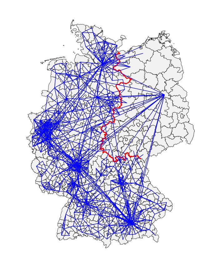
Figure 4a presents major outgoing commuter flows (more than 1,000 commuters per
county) originating in what used to be West Germany. We see that our expectation is
confirmed: almost all of them also go to the West. The only major destination in former
East Germany is Berlin (neither Dresden nor Leipzig receive significant inflows from the west
20
Large infrastructure projects try to overcome this pattern since reunification but it is, for example, still
difficult to reach Dresden from Cologne (or anywhere in the Ruhrgebiet) by public transport. Similarly,
the Berlin–Munich high-speed rail connection was under construction since 1996 and only achieved modern
speeds close to 4 hours in December 2017. Both distances are slightly less than 600 km.
17Figure 4 – Major commuting flows (at least 1,000 people) by origin
(a) Originating in west (b) Originating in east
Notes: Illustration of major commuter flows origination in the former FRG and former GDR based on
the December 2019 commuting flows published by the Federal Employment Agency (Bundesagentur für
Arbeit). For the purposes of this map, Berlin is geographically considered to be a part of the East.
but some counties on the eastern side of the old border receive some non-negligible flows).
Similarly, in Figure 4b we see that major outgoing commuter flows originating in former
East Germany also generally terminate in the East, again with the exception of significant
flows from the capital to other western major cities. This holds in spite of a large wave of
migration from East to West post-reunification. In fact, some of these flows are government
workers who officially commute between Bonn, the old capital of the FRG which retained
some government functions, and Berlin.
Table 5 puts these figures into our RD framework and presents discontinuity estimates
for the fraction of incoming commuter flows that originate in West Germany at the county-
level. Panel A shows that counties just to the east of the border receive between 32 and 72
percentage points more of their commuter flows from East Germany than do counties just to
the west of the border. The standard errors are relatively small, so that these estimates are
significant at all conventional levels. In Panel B of Table 5 we add this fraction of commuters
from the West to our baseline regression for COVID-19 cases per capita across all age groups.
This has a comparatively strong effect on the results. The RD coefficient at the reference
18Table 5 – Regression discontinuity results with commuting and simulated results
The dependent variable is log(1+cases/million)
The bandwidth is
50 km 75 km 100 km 150 km 200 km
(1) (2) (3) (4) (5)
Panel A. Fraction of incoming flows from West
East -.354*** -.475*** -.555*** -.669*** -.720***
(.027) (.026) (.022) (.020) (.021)
Panel B. Log(1+cases/million), controlling for flows from West
East -.544*** -.363** -.349* -.322 -.350
(.187) (.166) (.202) (.200) (.224)
Panel C. Log(1+cases/million), controlling for income, demographics and flows from West
East -.320 -.171 -.075 -.160 -.242
(.220) (.166) (.231) (.252) (.248)
Panel D. Log(1+simulated cases/million)
East -.438* -.493* -.588** -.866*** -.862***
(.227) (.254) (.235) (.245) (.222)
Observations 77 106 138 203 287
Notes: The table reports results from a regression discontinuity specification with an interacted
local linear RD polynomial and border segment fixed effects. Standard errors clustered on the state
(Bundesländer ) level are reported in parentheses.
bandwidth of 100 km falls by almost 0.5 log points and is only marginally significant at 10%.
At higher bandwidths, the effect is no longer significant at conventional levels. This is a
larger impact than controlling for log disposable income per capita, log population density
and the age distribution at the same time. In Panel C we also add log population density,
the age distribution as well as log disposable income (the controls from Panel E of Table 3).
Now the effect becomes numerically small at the reference bandwidth and insignificant for
the entire range of bandwidths. In other words, accounting for only differences in mobility
and demographics is enough for the discontinuity in cases to disappear.
Our final exercise demonstrates that mobility patterns, population differences and the
geography of the initial outbreaks can create a counterfactual discontinuity just like the
one we observe in the actual data. We simulate a canonical SIR model of the coronavirus
epidemic in each German county with mobility flows following Wesolowski et al. (2017) and
Bjørnstad and Grenfell (2008). In the model, we allow infections to spread along commuting
patterns starting from the distribution of coronavirus cases on February 29 2020 and use the
approximate epidemiological characteristics of the outbreak in Germany (e.g., a reproduction
number, R0 of 2.5). We use the observed commuting flows from December 2019 together with
19Figure 5 – Discontinuity in log(1 + simulated cases/million) at former border
14
13
12
11
10
-400 -200 0 200
Distance to the East of Former Border, kilometers
Notes: Illustration of the discontinuity log(1 + simulated cases/million people) across the former border
between West and East Germany. The simulation and its underlying parameters are described in
Appendix A. The figure shows non-parametric local polynomial estimates for bins of the dependent
variable, where each bin is 20 km wide. 95% confidence intervals are shaded in grey.
county population data to proxy for actual mobility around the time of the outbreak. We
simulate the model for 60 periods (days) but stop all commuting flows after 22 days to reflect
the nation-wide shutdown. The details of the simulation are provided in Appendix A.21
Panel D of Table 5 presents the discontinuity estimates for the simulated log cumulative
cases per capita. We find that in the simulated data, the number of cases also discontinuously
declines as one crosses from west to east over the former border. The decline is somewhat
smaller, but close in magnitude, to the decline observed in the actual data. This confirms
the results of the RD design with controls for commuter flows and strongly suggests that
mobility is a key driver of the geography of the early outbreak. Our methodology cannot
exclude other alternative explanations, and officially registered commuter flows likely do not
represent person-to-person movement across Germany perfectly. However, our simulation
constructs a situation that shares some essential features of the data, and that explains the
discontinuously lower novel coronavirus prevalence across the border into the former East
without reference to the (broad) BCG hypothesis. This fact together with the pattern in
the discontinuities across cohorts, leaves us very skeptical that the BCG vaccine plays a role
in explaining the geography of the outbreak in Germany.
21
The simulation overpredicts the overall case count because we do not explicitly model social distancing
(apart from the lack of commuting). In the observed data, the reproduction number declined toward unity
over the same period.
205 Conclusion
Our paper provides a cautionary tale of potentially misleading correlations, which appear
early in the outbreak of an epidemic. Using the modern applied econometrics toolkit, we
show that there is a stark break in cumulative COVID-19 cases at the former border which
used to separate East and West Germany. However, our analysis strongly suggests that
an appealing explanation—the variation in BCG vaccination status for large populations
across the border—cannot account for this discontinuity. Instead, more mundane factors
appear to be behind this East-West differences. Accounting for commuter flows, income
and demographics is sufficient for the difference to vanish. These results help to address the
identification problems encountered in the scientific and journalistic debate on the merits of
the BCG hypothesis.
Our findings have several important limitations. First, they are derived from the context
of Germany, the health profile of its population, and the specific strains of COVID-19
circulating there, and therefore may not be as applicable to other parts of the world. Second,
they cannot speak to the possibility of a short-run boost to the immune system coming from
the BCG vaccine that may offer individuals some “trained immunity” against COVID-19.
In particular, our results should not be taken to anticipate the outcomes of the clinical trials
that are currently taking place. Third, our study looks at a summary measure of the intensity
of the epidemic—cumulative case counts per capita—and does not consider in detail other
dimensions, such as the lethality of infections or the speed of transmission from the infected
to the susceptible.
While it is disappointing to find evidence against a partial remedy, we believe that
negative results are necessary for the world to redeploy resources in the right direction.
They also help guard against a false sense of security that countries with a current BCG
vaccination policy might feel. To the extent that current case counts around the globe
are a product of the early geography of the pandemic rather than of immutable features of
populations, less affected countries and regions should take their reprieve as a time to prepare
rather than as a time for complacency. It is not unimaginable that the raw discontinuity
we documented will eventually disappear or even turn around if the infection spreads to a
poorer, older and more disease-prone population in the East.
21References
Alesina, A. and N. Fuchs-Schündeln (2007). Goodbye Lenin (or not?): The effect of
communism on people’s preferences. American Economic Review 97 (4), 1507–1528.
Arts, R. J., S. J. Moorlag, B. Novakovic, Y. Li, S.-Y. Wang, M. Oosting, V. Kumar, R. J.
Xavier, C. Wijmenga, L. A. Joosten, et al. (2018). BCG vaccination protects against
experimental viral infection in humans through the induction of cytokines associated with
trained immunity. Cell Host & Microbe 23 (1), 89–100.
Asahara, M. (2020). The effect of BCG vaccination on COVID-19 examined by a statistical
approach: no positive results from the Diamond Princess and cross-national differences
previously reported by world-wide comparisons are flawed in several ways. medRxiv . DOI:
10.1101/2020.04.17.20068601.
Becker, S. O., L. Mergele, and L. Woessmann (2020). The separation and reunification
of Germany: Rethinking a natural experiment interpretation of the enduring effects of
communism. Journal of Economic Perspectives 34 (2), 71–143.
Berg, M. K., Q. Yu, C. E. Salvador, I. Melani, and S. Kitayama (2020). Mandated Bacillus
Calmette-Guérin (BCG) vaccination predicts flattened curves for the spread of COVID-19.
medRxiv . DOI: 10.1101/2020.04.05.20054163.
Bjørnstad, O. N. and B. T. Grenfell (2008). Hazards, spatial transmission and timing of
outbreaks in epidemic metapopulations. Environmental and Ecological Statistics 15 (3),
265–277.
Calonico, S., M. D. Cattaneo, and R. Titiunik (2014). Robust nonparametric confidence
intervals for regression-discontinuity designs. Econometrica 82 (6), 2295–2326.
Covián, C., A. Fernández-Fierro, A. Retamal-Dı́az, F. E. Dı́az, A. E. Vasquez, M. K.-L. Lay,
C. A. Riedel, P. A. González, S. M. Bueno, and A. M. Kalergis (2019). BCG-induced cross-
protection and development of trained immunity. implication for vaccine design. Frontiers
in Immunology 10, 1–14.
Curtis, N., A. Sparrow, T. A. Ghebreyesus, and M. G. Netea (2020). Considering BCG
vaccination to reduce the impact of COVID-19. The Lancet.
Dell, M. (2010). The persistent effects of Peru’s mining Mita. Econometrica 78 (6), 1863–
1903.
Deshpande, M. (2016). Does welfare inhibit success? The long-term effects of removing low-
income youth from the disability rolls. American Economic Review 106 (11), 3300–3330.
Fuchs-Schündeln, N. and T. A. Hassan (2015, June). Natural experiments in
macroeconomics. Working Paper 21228, National Bureau of Economic Research.
Gelman, A. and G. Imbens (2019). Why high-order polynomials should not be used in
regression discontinuity designs. Journal of Business & Economic Statistics 37 (3), 447–
456.
Genz, H. (1977). Entwicklung der Säuglingstuberkulose in Deutschland im ersten
Jahr nach Aussetzen der ungezielten BCG-Impfung. DMW-Deutsche Medizinische
Wochenschrift 102 (36), 1271–1273.
Harsch, D. (2012). Medicalized social hygiene? Tuberculosis policy in the German
Democratic Republic. Bulletin of the History of Medicine 86 (3), 394–423.
Imbens, G. and K. Kalyanaraman (2011). Optimal Bandwidth Choice for the Regression
22You can also read