The study of electromagnetic processes in the experiments of Tesla
←
→
Page content transcription
If your browser does not render page correctly, please read the page content below
The study of electromagnetic processes in the experiments of Tesla

                                    B. Sacco1, A.K. Tomilin 2,
                      1
                          RAI, Center for Research and Technological Innovation
                                      (Turin, Italy), b.sacco@rai.it
                            2
                             National Research Tomsk Polytechnic University
                           (Tomsk, Russian Federation), aktomilin@gmail.com

       The Tesla wireless transmission of energy original experiment, proposed again in a downsized
scale by K. Meyl, has been replicated in order to test the hypothesis of the existence of electroscalar
(longitudinal) waves. Additional experiments have been performed, in which we have investigated the
features of the electromagnetic processes between the two spherical antennas. In particular, the origin
of coils resonances has been measured and analyzed. Resonant frequencies calculated on the basis of
the generalized electrodynamic theory, are in good agreement with the experimental values found.

       Keywords: Tesla transformer, K. Meyl experiments, electroscalar            waves, generalized
electrodynamics, coil resonant frequency.

          1. Introduction
      In the early twentieth century, Tesla conducted experiments in which he
demonstrated unusual properties of electromagnetic waves. Results of
experiments have been published in the newspapers, and many devices were
patented (e.g. [1]). However, such work has not received suitable theoretical
explanation, and so far no practical application of the results have been
developed.
     One hundred years later, Professor K. Meyl [2] aimed to reproduce the
same experiments using a miniature, laboratory version of the Tesla setup,
arguing that it can help to detect unusual phenomena that are explained by the
presence of electroscalar (longitudinal) waves, namely:
       • the reaction on the transmitter of the presence of the receiver;
       • the transmission of scalar waves with a speed of 1,5 times the speed of
           light;
       • the inefficiency of a Faraday cage in shielding scalar waves, and
       • the possibility of wireless transmission of electrical energy.
     Nearly ten years have passed since the publication of the results of K. Meyl
experiments. However, despite this, they still have not received a clear
theoretical explanation. Some authors, for example [3], believe that the observed
phenomena can be explained on the basis of the properties of ordinary transverse
electromagnetic waves. It has been suggested that the set-up of K. Meyl does not
play all the experimental conditions of Tesla.
     Are there really unexplored components of the electromagnetic wave?
Under what conditions do they occur? Which are their properties? These are
important questions that remain open. From the answers depend our assessment
of the current state of electrodynamics and science in general. In this situation it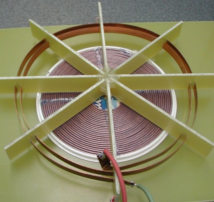
is needed a balanced and pragmatic approach allowing to take into account all
the correct facts and give them the correct interpretation.
     The relevance of setting and study the issues raised above is now obvious.
There are a lot of experimental facts and theoretical considerations that require
interpretation. The so-called electroscalar waves have been observed in the
experiments carried on by C. Monstein and J. P. Wesley [4], and by G.V.
Nikolaev [5]. Theoretical substantiation of the physical meaningfulness of the
electroscalar waves is contained in N.P. Hvorostenko [6], A.K. Tomilin [7-9],
Koen J. van Vlaenderen [10], D.A. Woodside [11]. The problem of
experimental detection electroscalar waves is also dealt with by G. Bettini [17].
Interesting results are contained in the Elmore G. paper [18].
      This work includes experimental and theoretical parts. The basic K. Meyl
experiments have been reproduced, and supplemented with new experiments to
detect and describe the phenomena that cannot be explained on the basis of
modern electromagnetic field theory. The included theoretical analysis is based
on a generalized theory aimed to complete the modern electrodynamics for
encompassing all known (including the little-studied) experimental facts and
natural phenomena.

     2. The K. Meyl experiments summary
      The system originally proposed by Tesla [1] (Fig. 1) consisted of a
transmitter including a resonant transformer with a strong elevation of potential:
the high inductance spiral secondary coil, loaded by a low capacitance
“elevated” metal sphere, was coupled to a low inductance spiral primary coil1.
The transmitter primary was driven by a high frequency, high voltage supply.
The receiver was identical and symmetrical. The load was e.g. a set of lamps
connected in parallel at the receiver output. As affirmed by Tesla himself, the
ground connection in this structure plays an important role.
      With this structure Tesla did actually demonstrate something that today
would be unthinkable to be done with Hertz radio waves: in Colorado Springs
he built two towers, one 10 kW transmitter and a receiver located at a distance of
25 miles, and he demonstrated that it could be receive substantially 100% of the
transmitted power, in facts, he could power 200 fluorescent lamps of 50 watts
each. The experiment was published in the contemporary newspapers.
      K. Meyl [2] experiment is inspired by Nikola Tesla patent mentioned
above. In fact, the structure used is a miniature version (but not on scale) of the
receiver and transmitter towers of the original installation of Tesla. Here,
however, the size of the "towers" is about thirty centimeters. Each tower has a
flat Tesla coil in its base plate, consisting of a two turns spiral primary coil and a
many turns spiral secondary coil, made on a single printed circuit board. A

1
 In some implementations by Tesla himself, the primary was brought to resonance adding
high-capacity capacitors in parallel.
sphere with metal surface is placed on top, connected by a wire to the inner end
of the secondary.

                                        Fig. 1

     In order to make precise measurements of frequency, Meyl adopted a small
synthesized frequency generator with digital readout. Due to the relatively small
size of the equipment, the frequency range of the resonance that results is in the
order of a few MHz, while Tesla was working at frequencies much lower. In
addition, these small-scale demonstration devices are fed with signals voltage of
about 2 V, while Tesla, in his great power wireless transmission installation,
used about 60 kV supply (the antenna potential being much higher).
     In Fig. 2 is outlined the structure adopted by Meyl. The RF generator is
connected in parallel to the primary of the Tesla Coil (TC) transmitter, two
LEDs in anti-parallel are connected across TC input too. The TC secondary is
isolated from the primary. The inner end, as already mentioned, is connected to
the metal ball; the outer one is connected to the "earth", which in this experiment
is emulated, in a "degenerate" way, with a single copper wire that reaches the
receiver.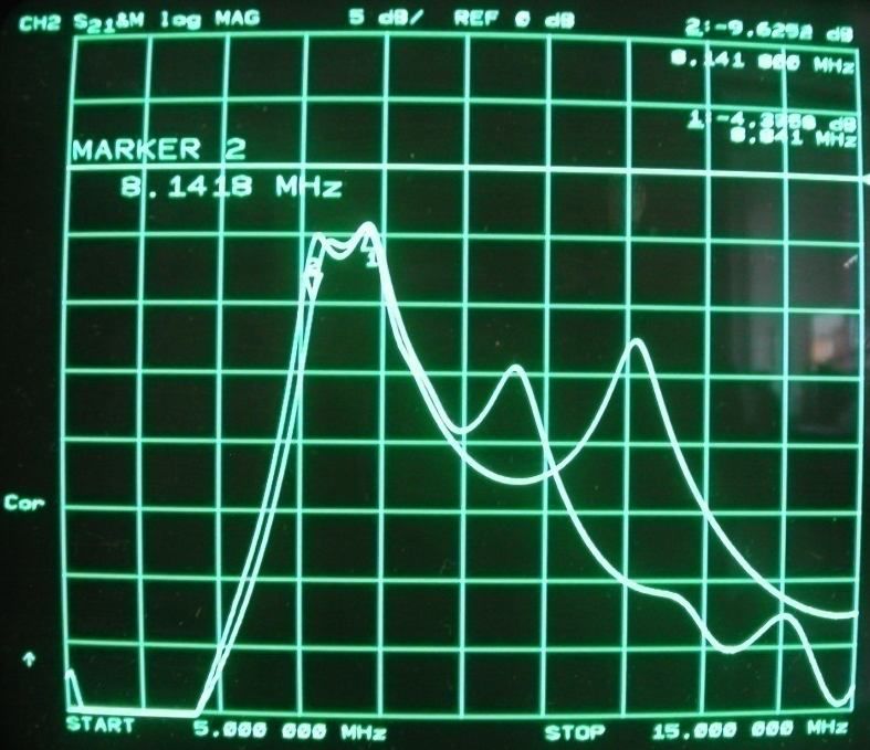
Fig. 2
The transmitter and receiver are completely symmetric. As a "load" two
LEDs are connected in anti-parallel, symmetric and similar to those present at
the transmitter. Photo set K. Meyl shown in Fig. 3.
Fig. 3
In his experiment, K. Meyl has adopted the following procedure:
• First step: The output level of the generator set to approximately 2V. The
generator frequency is adjusted, until the resonant frequency are detected by the
brightness of the LEDs on the receiver. The [main, higher] resonance is found at
a frequency f 02 7МHz . At the resonance, the transmitter LEDs turn off.
• Second step: Then the receiver earth wire is disconnected. In this case the
receiver LEDs are extinguished and the transmitter will light up brightly. That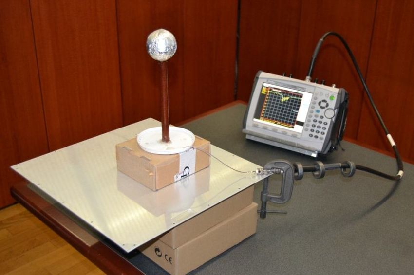
is, the transmitter "feels" if the receiver receives the signal. K. Meyl called it "a
reaction to the receiver back to the transmitter."
• Third step: tuning down the frequency, another resonance is found at
f01 4,7МHz ; here the receiver LEDs are less shining, and the signal is easily
screened. The reverse reaction of the transmitter to the receiver is absent.
Professor K. Meyl interprets the phenomena described above as follows.
In the first step of the procedure, adjusting the frequency generator to the
appropriate frequency, it results:
a) receiver LED lights up. Meyl interpretation: "In this condition the
energy transfer takes place”;
b) simultaneous fading down of the transmitter's LED. Meyl
interpretation: “Back-reaction of the receiver on the transmitter”.
In the second step of the procedure, the transmitter LED lights again, when
the operator disconnects the receiver. Meyl interpretation: “This is a proof of the
back-reaction of receiver on the transmitter”.
In the third step, for the resonance at lower frequency, f 01 4,7МHz , it is
highlighted that occurs:
a) lower intensity of the LED,
b) signal can be easily shielded,
c) lack of marked back-reaction on the transmitter.
Meyl interpretation for points a,b,c above: “This is conventional, Hertzian
waves. This is a proof that scalar waves speed (for resonance at 7MHz) is
higher than the one of Hertzian waves (resonance at 4.7MHz). In particular,
scalar waves speed results 7/4,7=1,5 times the speed of light2”.
3. Replication of the K. Meyl experiments and discussion
3.1 Basic replication
The K. Meyl experiment has been replicated in the laboratory of the Rai
Research and Technological Innovation Cent (Italy). From the cited paper not
the all parameters of the TC are disclosed, but, under the likely hypothesis that
from the geometrical dimensions will depend only the resonance frequencies,
not the overall behavior of the system, it was decided to proceed building two
pairs of coils with size roughly similar to the Meyl’s ones, thus accepting some
uncertainty margin.
We used a standard sinusoidal signal generator HP33120A. As indicators,
the LEDs were first used. Initially, the entire apparatus was placed on the bench,
the distance between transmitter and receiver being quite limited (approximately
0.5 m).
2
No explanations is given in the paper.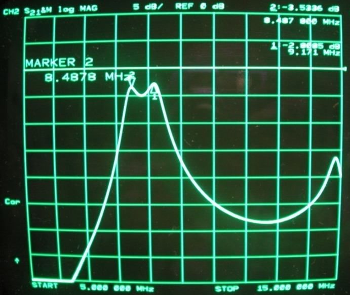
Transmitter
Primary
Winding type Counter-clockwise spiral
Number of turns 2 turns
Wire type Copper ribbon, 8mm x 0.5mm
Inner diameter 150mm
Outer diameter 163mm
Secondary
Winding type Counter-clockwise spiral
Number of turns 31 turns
Wire type coax cable, 1.3mm diameter (1.7mm including outer
insulation; outer + inner conductors used together as
single conductor)
Inner diameter 10mm
Outer diameter 117mm
Antenna
Pole Bakelite tube, l= 195mm with internal wire.
Sphere 63mm polystyrene sphere coated with aluminium foil
Receiver
Primary
Winding type clockwise spiral
Number of turns Same as Tx
Wire type Same as Tx
Inner diameter Same as Tx
Outer diameter Same as Tx
Secondary
Winding type clockwise spiral
Number of turns Same as Tx
Wire type Same as Tx
Inner diameter Same as Tx
Outer diameter Same as Tx
Antenna
Pole Same as Tx
Sphere Same as Tx
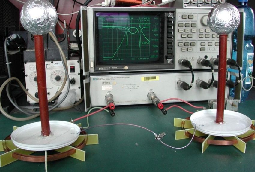
Both helical coils (primary and secondary) are shown in the photograph
(Fig.4).
Fig. 4
The first step: The generator output level is set approximately 2V. The
oscillator frequency is adjusted until the LED on the receiver will shine brightly.
This corresponds to the resonance frequency f 02 .
The above statements have been verified; in our experiment, as expected,
the resonance frequencies f 02 differ from experiment K. Meyl because of the
size of the coils. The values found are: f 02 11,27МHz .
The second step: Grounding the receiver is disconnected. Then, the
receiver LEDs turn off and the transmitter LEDs turn on again. Thus, as if the
transmitter "feels" that the signal has been received by the receiver ("the reaction
of the transmitter to the receiver"). The above statements have been verified.
In the third step we found the expected resonance at lower frequencies.
The frequency found is: f 01 8,5МHz . Instead, the less clear "reaction" back on
the transmitter at this lower frequency is not evident.
3.2 Discussion of the basic phenomenology
Phenomenon 1: The transmitter LED is "normally" on. (except in special
circumstances). This behavior is easily explained, noting that the LED is in
parallel with the same RF generator, so it is normally powered by the latter.
Phenomenon 2: By adjusting the frequency of the generator there is a
value (8.5 MHz, see above) in which the receiver LED lights up.
This effect is of course indicator of preferential transfer of energy from the
transmitter to the receiver. The fact that this happens at a given frequency
indicates the presence of a resonance, which in facts is verified instrumentally
with other methods, as mentioned below. If we increase the power of RF
generator, the range of LED lighting widens as one would expect under the
assumption of resonance.
The most important question is: which way energy is transmitted from the
transmitter to the receiver? Two hypotheses can be proposed. The first one
assumes that some sort of electromagnetic process is conveying the energy in
the space between the spherical antennas. The features of such process are to be
identified. Obviously, the usual capacitive coupling must be ruled out in this
case, since this phenomenon, as mentioned below, is observed at large distances
between the emitting and receiving antennas. In this sense, the radiating antenna
is used as an energy source, and the receive antenna as an energy sink. But we
cannot ignore, as a second hypothesis, that energy transfer can occur through the
ground cable. We will carefully examine each of the assumptions made.
Phenomenon 3: At about the same frequency, or at least in a small range
almost coincident, the Tx LED will turn off (or fade if the RF generator power is
too high).
This effect is less intuitive. By use of instruments, we saw that the
weakening of the signal on the transmitter LED is determined by the fact that the
impedance seen at the transmitter primary - which is obviously a function of
frequency - has a low value resistive component at the resonance frequency.
Phenomenon 4: When disconnecting the ground from the receiver, its light
is extinguished and the transmitter LED goes on again.
Under the first of the hypothesis, this "reaction of the receiver on the
transmitter" can be explained as follows: when disconnecting the receiver from
ground, its reactance parameters changes and breaks the resonant mode of
energy transfer between spherical antennas. As a result of sharply reduced level
of energy absorbed by the receiver (the receiver LED goes off), the energy is no
longer transferred from RF generator to the Tx, due to impedance mismatch; as
a consequence more energy is available for the Tx LED (transmitter LED lights
up).
The second hypothesis explains this phenomenon as the cessation of
transmission of energy through the ground cable from its attachment to the
receiver. For the same reason as above, the Tx LED have more energy again,
and it lights up.
Phenomenon 5. Between the two spheres is inserted a grounded metal
screen 30 40cm . No significant attenuation of the received signal has been
detected at both resonant frequencies. There is only a slight shift of the
resonance frequencies.
If we assume that energy transfer occurs through a process between
spherical wave antennas, it is necessary to conclude that it has properties
different from properties of Hertzian waves. Again, this behaviour is
compatible with the hypothesis of the signal transmission through the ground
cable.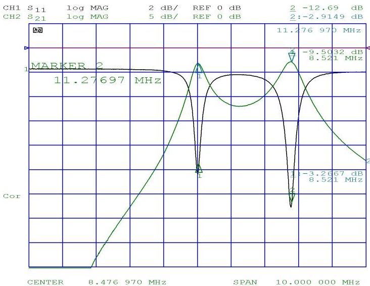
The experiments described above is not sufficient to unambiguously
interpret the observed phenomena, and therefore have been produced additional
experimental studies.
4. Additional experiments
4.1 Frequency response of the system
The availability of suitable laboratory equipment has allowed a detailed
study of the global behaviour of the system in a frequencies range of 0-30MHz.
For analogy with Meyl original resonance frequencies, in subsequent analysis
we will refer to as f 01 and f 02 for the first and second resonance frequencies
respectively, though the values will be somewhat different.
We used a Vector Network Analyzer (VNA) Agilent HP8753B and,
equivalently, an Anritsu MS2026C, depending on laboratory availability.
Fig. 5
The instrument was set in S21 mode, to display the frequency response of
transmission from port 1 to port 2, and was calibrated. Port 1 of the VNA was
then connected to the transmitter, and the output of the receiver was connected
to port 2 of VNA (Fig.5). The transmission (from input to output) is
characterized by the dimensionless (in decibels) S21 parameter, defined as:
B2
S21 10 log .
A1
where B2 is the power wave outgoing from Port 2 and A1 is the power wave
incoming in Port 1.
The input reflection parameter, S11 is defined as:
B1
S11 10 log .
A1
where B1 is the power wave reflected back from Port 1 and A1 is the power wave
incoming to Port 1.
Fig. 6
In the analysis of transmission amplitude-frequency characteristics, two
resonances are visible (Fig. 6):
• the first at frequency f 01 8,52MHz S21 3,2dB
• the second at frequency f 02 11,27MHz S21 2,9dB .
Since, as mentioned, the black curve S11 describes (in decibels) the ratio
of the power reflected back to the instrument’s generator, over the forward
power incident on the device input, a low value indicates low reflected power,
therefore much power transmitted to the device. As a consequence, this
indirectly describes the current in the indicator circuit of the transmitter. It canbe seen, as expected, that each resonance minimum S11 also corresponds to the
of the maximum energy released in the load receiver, as shown by trace S 21 .
The peak value of the received signal at a frequency f 01 is lower than the
one at frequency f 02 . This is consistent with the fact that Meyl notes: "By
lowering the frequency of the signal indicator lights up the receiver again, but
with less intensity."
Fig. 7
The following experiment was performed with the transmitter only (the
receiver being totally disconnected); we investigated the input reflection
parameter, S11 versus frequency of the transmitter alone in the frequency range
from 0 to 60 MHz. As visible in Fig. 7, three resonance peaks are present, at
frequencies: f 011 9 MHz S11 7,77 dB , f 021 30 MHz S11 1,86 dB and
f 031 45,6MHz S11 2,52 dB .
Obviously, comparing with the full system S11 behaviour (Fig. 6), the third
peak is outside the frequency range and therefore not visible. In addition, we
note that in an experiment with a solitary transmitter first resonance peak has
shifted slightly, and the second resonant frequency is substantially increased.
This means that the presence of the receiving system has a strong influence on
the electromagnetic parameters of the process at a frequency of secondresonance peak. This again points to the distinguishing features between the
electromagnetic processes occurring at different frequencies. It is also needed to
explain the cause of resonance at the three frequencies where peaks occur.
4.2 Phase relationships at resonances
For this test, the complete system (transmitter and receiver) has been
operated at a fixed frequency. Two probes of the oscilloscope (yellow and green
lines in Fig.8a and Fig.8b) were placed at short distance (3-4cm) from the
spheres, to sense the electric field. The third probe (blue trace) was close to the
“ground” wire.
At f 01 8,52MHz (Fig.8a) signals on the transmitting and receiving
antennas differ in phase by 180 degrees. The signal on the “ground” wire has an
intermediate phase. Note its very low level.
Fig. 8a Fig. 8b
A
At f 02 11,27MHz signals on both antennas have the same phase (Fig. 8b).
The signal in the “ground” wire is in counter-phase, and its level is very high.
All this confirms that the electromagnetic process at each resonant
frequency has its own distinctive features.
4.3 Interpretation of the behaviour at the resonances
The above results are consistent with the model of the wire dipole antenna.
For the resonance at f01 8,52MHz, in a dipole antenna with size equal to half the
wavelength, (without any extra inductance and capacitance) the canonical
voltage distribution is the one shown in Fig.9a.
In the presence of capacitive elements at the ends (Top loaded antenna
dipole or Hertzian dipole), the geometric length of the dipole is reduced for the
same resonance (Fig.9b). By adding an inductive load (Fig.9c) the geometric
length of a dipole at the same resonance, is further reduced. From this diagram
we see that: on the inductor, there is a jump of the charge (as well as potential);
the terminal points of the dipole have potentials of opposite sign: they
oscillate in opposite phase, as in the experimental waveform in Fig. 8a;
the voltage in the middle point is theoretically zero (undefined phase,
then), in good agreement with observed very low voltage on the “ground
wire” (waveform of Fig. 8a, purple trace). Since the magnitude is
nominally zero, the phase is unimportant here.
Fig. 9
We now consider the next resonance frequency (second overtone,
f 02 11,27MHz ). A common / 2 dipole would have the voltage distribution of
Fig.10a. The capacitive load at the ends (Top loaded antenna dipole or Hertzian
dipole) shortens the geometric length the dipole at the same resonance as shown
in Fig.10b. The same considerations already mentioned apply. When adding an
inductive load (Fig.10c), the geometric length of the dipole for the same
resonance is further reduced. From this diagram we see that:
on the inductor, there is the jump of the charge, as above, which leads to
considerable increase of the voltage; the ends of the dipole have the same potential, therefore they oscillate in-
phase (in agreement with Fig.8b, yellow and green traces);
in the middle point the potential is very high and is in antiphase with
respect to end potentials (as experimentally observed: Fig.8b, purple
trace).
Fig. 10
4.4 Upper resonances in the individual Tesla Coil
An attempt has been made to visualize the resonances of the basic Tesla
Coil (solitary transmitter) on a wider frequency range: 0 to 300MHz.
In order to avoid spurious resonances from the feeding cable itself, three
EMI-type (dissipative) ferrite toroid cores have been inserted on the cable.Fig. 11
Fig. 12
The frequency response of energy absorption (Fig. 11) shows that the main
resonance occurs near 160 MHz and has three peaks at frequencies
f1 141,7MHz [Marker 1], f 2 161,5MHz [Marker 2], and f3 179,8MHz
МК3[Marker 3]. The observed initial response in the short wave is obviously not the
main, the waveform shown on the left it shows the first peak.
4.5 Transmission loss versus distance
This series of tests studied the trend in the attenuation of the signal versus
the distance between the transmitter and receiver. The transmitter and receiver
were placed on wooden pedestals. They could be moved in the corridor of the
building. The VNA analyzer was placed near the receiver. A 20-meter long
coaxial cable (RG213, 50 Ohm) has been used to connect the VNA output to the
transmitter. The “ground wire” had a length of 20 m too. Both cables length
were not changed during the experiment3.
4.5.1 Test at a distance 1 m
At 1-meter antennas distance the resonance peaks shifted somewhat
compared with the previous bench tests, in which the distance between the
antennas was less than 50 cm. As expected, the ground wire length of 20 m,
extending from the transmitter to the analyzer, affects the resonant frequency,
reducing it: f 01 7 ,9 MHz , f 02 8,7 MHz , f 03 10 ,8 MHz . Attenuation at
this frequency f 02 8,7MHz is approximately S21 3,8dB.
4.5.2 Test at a distance 4 m
Losses at resonance f 02 8,7 МHz of slightly increased: S 21 4,4dB (Fig.13).
Fig.13
3
Note that, with respect to theoretical analysis (section 5.6 below) the resistance R would increase only with
additional cable added; the resistance R remains unchanged. The obvious result is the relation: R RIt was observed that the frequency response significantly depends on the
position of the grounding cable. Two tracks on the oscilloscope screen are
examples of two different provisions of the grounding cable. The only
unchanged point is the one corresponding to frequency 8.7MHz. An explanation
of this fact is given in the theoretical analysis section below.
4.5.3 Test at a distance 15 m
The degree of attenuation at the resonant frequency f02 8,7MHz (marker
1) remains unchanged: S 21 4,4dB . At off-resonance frequencies, on the
contrary, there are significant attenuations of the signal (Fig.14). (Note: vertical
scale is 5dB per division). The second trace (memorized) is the previous test, for
comparison.
Fig. 14
4.5.4 Test at a distance 18 m (Through concrete wall)
In this test the line of sight was blocked by a concrete wall (Fig.15).
Compared with the previous test, no difference has been observed: the resonance
frequency f 02 8,7MHz the path loss remains the same: S 21 4,4dB .Fig. 15
The observed dependence of the attenuation at f 02 8,7 МHz versus distance is
summarized in the table below:
Distance [m] Path loss [dB]
1 -3.8
4 -4.4
15 -4.4
18 -4.4
At a distance of over 4m energy of the transmitted signal at a
frequency f 02 8,7 MHz is stabilized. Such a decay law of the received signal as
a function of the distance between the transmitter and the receiver is anomalous.
As noted above, in the experiments on signal transmission between the
spherical antenna done by C. Monstein and J. P. Wesley [4], the transmitted
signal faded as the square of the distance from the radiation source. Such
dependence is a normal distribution with a spherical electromagnetic wave.
In contrast to C. Monstein and J. P. Wesley set-up, here the Tesla and K.
Meyl antenna contain spiral coil. Perhaps the anomalous decay law of the signal
energy due to processes occurring in the Tesla transformer. This phenomenon
requires further study.
4.6 Transmission through a Faraday Cage
In the analysis of the observed phenomena it has been repeatedly raised the
question: is the energy transmitted from the transmitter to the receiver solely on
ground conductor? In other words: is there a signal (energy) transmission path
directly between the spherical antennas by electromagnetic waves? And whatare the properties of these waves? It has been therefore tried to analyze this
phenomenon more accurately using a professional Faraday cage (Fig.16).
Fig. 16
The transmitter was placed in the Faraday cage, mounted on a wooden table, and
it was fed from the outside (VNA, port 1) by a coaxial cable through the cage
connectors panel.
Fig. 17
The receiver was placed outside the cage on a wooden pedestal. The
received signal was fed to the VNA analyzer port 2 (Fig.17).
4.6.1 Case1: ground cable is insulated
In the first test the ground wire from the transmitter was brought outside
the cage through a small insulated hole in the metal wall (Fig. 18). The hole was
about 8 mm in diameter, that is much smaller than the wavelength, so it should
not affect the shielding of radiated signals.Fig. 18
Fig. 19
The cage door was first kept open, the transmitter and receiver being in the
line of sight. Then, under the same conditions above the chamber door was
closed.
Surprisingly, no difference was found: in Fig. 19 the two curves (with the
door open and door closed) are identical, perfectly overlaying.4.6.2 Case2: ground wires connected to the Faraday cage
The experiment was repeated with the same configuration as above, but the
ground wire of the transmitter was electrically connected to the inner side of the
cage metal wall, and the ground wire of receiver to the outer side of the cage
metal wall (Fig. 20).
Fig. 20
Under these conditions, as before, there should be no obstacle on the
ground conductor for a signal transmission from the transmitter to the receiver.
However, in this case, the attenuation of the signal was found very high (high
shielding effectiveness).
5.Theoretical analysis
To better understand the phenomena observed in the above experiments, it
is necessary:
• to investigate the electromagnetic processes that take place between the
transmitter and the receiver and find out their features;
• explore the possibility of transmission of the signal (energy) over great
distances.
• to find out a theoretical model able to describe the resonances observed;
From the standpoint of the modern theory of electromagnetic waves, the
results of the experiments described above seem quite paradoxical. Theobserved phenomena are obviously beyond the traditional concepts of the
electromagnetic process. Hereafter we will refer to the generalized (four-)
electrodynamics [7-9], which, as we will see, covers a wider range of
phenomena.
5.1 The wave equations
In the macroscopic description, the theory of electrodynamic processes
reduces to the well-known wave equations for the four-dimension vector-
potential A, :
2A
A 2
j , (1)
t
2
2
, (2)
t
where and are respectively the dielectric permittivity and magnetic
permeability, j and are the current density and charge density.
Introducing the four-dimensional space-time,
x1 x, x2 y, x3 z, x4 ict
we can write the corresponding components of the vector potential as
1 Ax , 2 Ay , 3 Az , 4 ic ,
and the four-wave equation that combines (1) and (2):
s , 1, 2,3, 4 . (3)
Here - is the invariant d'Alembert operator, and it is used a four-component
current density vector:
s1 Vx , s 2 V y , s3 V3 , s 4 ic.
Let us consider the resulting four-dimensional divergence of the vector-
potential:
1 2 3 4
divA . (4)
x1 x 2 x3 x4 t
Typically, from mathematical considerations, this expression is assumed to be
equal to zero, that is, it is apply the Lorentz condition. Disadvantages of thisapproach are shown in the studies [7-9]: it is proposed to abandon the terms of
Coulomb and Lorentz and assume the relationship:
B* x, y, z, t divA
, (5)
t
where B * x , y , z , t is a scalar function that characterizes an additional
component of the magnetic field. In the stationary case:
B * x, y , z divA . (6)
In the publications [7-9] it is theoretically and experimentally shown that
the potential (scalar) component B* of the magnetic field has a full physical
meaning. Also discussed are the conditions under which there is a potential
magnetic field. It is shown that the electric current in presence of an external
potential magnetic field, experiences a force directed along the current or
against it, depending on the sign of function B * x, y , z . In said publications the
irrotational law of electromagnetic induction is theoretically and experimentally
substantiated: it is shown that in a conductor placed in a time-dependent
potential magnetic field it is induced an electric field potential.
It follows that, for a complete description of the magnetic field it is
required to use the four-vector B, B* , which reflects its potential-vortex
character. Thus, failure of Coulomb calibration, allows to consider both
potential and vortex components of the vector A . This implies a generalized
field theory. We formulate the fundamental theorem of Helmholtz (Stokes) [12]
applied to the vector A : if the divergence and the curl of the field, vanishing at
infinity, is defined at each point r in a certain region, then everywhere in this
region the vector A field can be uniquely represented as the sum of potential
and solenoidal fields:
A A A .
5.2 Electrodynamic properties of the vector potential
Usually the Helmholtz theorem is not directly applied to the vector
magnetic potential A , because the latter is considered just a support function
and it is not uniquely determined. Let us examine the properties of the vector A .
In classical electrodynamics are used the following equations:
A
В rot A , E grad. (7)
t
and typically it is used the following gauge transformation:
A A grad , , (8)
t
where - is an arbitrary scalar coordinate-time function. The characteristics of
the vortex magnetic field, E , D and B, H of the induced electric fields, are
invariant under the transformation (8). On this basis it is concluded the gauge
invariance of the electromagnetic field. This is the basis for the introduction of
the Coulomb gauge and Lorentz condition. No physical meaning to the
transformation (8), is usually, not given.
Let us try to explain physical meaning of gradient transformation. Note
that by adding grad to the vector potential, its potential part changes.
Potential part of a vector field changing without vortex component’s changing is
possible only in the transition from conventional fixed reference frame К to a
steadily moving reference frame К . But in this case, obviously, potential part
of the electric field in the direction of the reference system must change. In
moving reference frame the electric field of a point charge is not spherically
symmetric, but appears Heaviside ellipsoid [13]. To compensate this change
(“deformation”), an additive with a minus sign is introduced to the second
t
correlation. Does the scalar potential really change at the transition from K
to К ? It is known [13] that the charge is relative invariant value. Scalar
potential depends on the location of the point of its definition and the
magnitude of the charge, therefore, there is reason to consider it in all reference
frames the same (at К speeds much smaller than the speed of light).
"Deformation" of the electric field in the transition to the mobile reference
system is fully taken into account by vector potential А . That is, there is no
need to introduce a second correlation (8), it has no physical meaning. To
describe the transformation of the electric field in the transition between K and
К (gradient transformation) only the first relation (8) is necessary.
There are two types of transformations of the vector field А: gradient and
vortex. Gradient transformation, as has been shown above, corresponds to the
transition between progressively moving reference frames (one of them can be
considered relatively immobile). When vortex transform, corresponds to a
transition from progressively moving (or conditionally stationary) reference
frame К to the rotating К .
It can be shown rigorously [7] that upon gradient transformation the
potential characteristics of the electromagnetic field ( A, and, consequently, Е
*
and В ) will change, while vortex characteristics ( A ,and, consequently Е
and В ) are invariants. Upon vortex transformation, on the contrary, vortex
components of the electromagnetic field do change, and potential ones are
invariants. This corresponds to the relative nature (depending on the choice of
the reference frame) of the magnetic field and its basic characteristics -vector А : in other words, the correlation of solenoidal and potential components
of the electrodynamic vector А depends on the choice of the reference system,
but in the selected reference frame is uniquely determined. Information
contained in brackets in the Stokes-Helmholtz theorem, merely reflects the
relative character of motion (rest) of any reference system. In selected arbitrarily
fixed reference frame it is convenient this vector constant equal to zero. In this
approach, the ambiguity of the choice of potentials А and disappears, and
there is no need to introduce gauge conditions. A theory formed on this
platform will be called generalized electrodynamics.
5.3 Modified (generalized) Maxwell's equations
From wave equations (1) and (2) with the relations (5) and (7) we can
easily obtain the generalized equation of electrodynamics (Maxwell's modified
equations) [7-9]:
D
rotH gradH * j
t , (9)
*
B
divD 0
t . (10)
This approach does not allow to exclude from these equations the potential
(scalar) component of the magnetic field, which is described by two interrelated
scalar functions:
B * H * . (11)
To denote the components of the magnetic field will use hereafter the term
"scalar magnetic field" (SMF).
The equations of the generalized electrodynamics (9) - (10) take account of two
D B *
non-stationary process: bias current and 0 , which can be called
t t
"Charge-shift". The presence of a charge-shift due to the phenomenon of
irrotational electromagnetic induction, has been confirmed experimentally [7].
Its essence is that of an unsteady SMF-induced electric field potential. Hence, a
“quasi charge”.
Another two differential equations that complement the generalized
electrodynamics, are (7):
B
rotE , (12)
t
divB 0 . (13)
Equation (12) describes the phenomenon of electromagnetic eddy
induction. In Maxwell's electrodynamics we consider only the eddy time-
dependent processes. The generalized electrodynamics describes, in addition,time-dependent processes that give rise to the potential components of electric
and magnetic fields. If these transients are created by third-party generators,
they are the real sources of the electromagnetic field. Instead, in the case of the
free field at any given point in time should be considered as quasi sources.
Equations (9) - (10), (12) - (13) and of their individual functions describe
electromagnetic phenomena, and for a complete description of the
electrodynamic processes we must also use the wave equation (1) - (2) and the
main electrodynamic characteristics, the 4- dimensional vector potential А, .
In papers [7-9], the potential component of the magnetic field was studied
theoretically and experimentally. A particularly useful formula (14) allows to
determine the intensity of the SMF, the created by the current J of finite length
(Fig. 21):
L
J zdz J r1 r2 J (14)
H x ,y ,z
*
sin 2 sin 1 .
4
0
r 3 4 r1 r2
4r0
x
M x , y , z
r1 r2
r0
1 2 z
O
L
y
Fig. 21
In Fig. 22 presents the line of the vector potential А and magnetic field
*
vector H and scalar magnetic field H created by a straight current segment of
finite length.
x
H* А H*
А
0 L z
H
y А
Fig. 22Based on the results of studies [7-9], we can formulate the rule: looking
from the midpoint of a finite-length current element, towards the direction of
current flowing in it, it is created a positive SMF ahead, and a negative SMF
behind. Note that the SMF in its essence is always heterogeneous and spatially
unrestricted (i.e., it vanishes at infinity).
5.4 Wave processes
From equations (1) - (2) using the second relation (7) we can easily obtain
the wave equation:
2E j 1
E 2 grad . (15)
t t
Conduction currents can be separated into radial j and azimuthally j
components. With this in mind, it is now possible to split (15) into two
independent equations:
2E j 1
E 2
grad , (16)
t t
2E j
E . (17)
t 2 t
Similarly, using the first relation (7) from (1) - (2), we obtain the wave
equation for the vector H :
2H
H 2 rotj . (18)
t
Equations (17) and (18) describe the well-known mechanism of the
emission of transverse electromagnetic waves.
Similarly, transforming (1) - (2) with (6), we obtain the wave equation for
*
a scalar function H :
* 2 H *
H 2
divj . (19)
t t
The differential equations (16) and (19) together describe the propagation
of waves along the irrotational vector Е , so they should be called the
longitudinal or electroscalar [10, 15].
It is important to note that, since the vortex and potential components of
the corresponding fields are mutually independent, equation (16) - (19) are fully
consistent with the principle of superposition. The sources generating potential
and vortex fields are respectively separated. However, there is a question of
mutual communication between non-closed conduction currents and charges,which reflects the condition of continuity. In Maxwell's electrodynamics is used
as a continuity condition:
divj 0 . (20)
t
Let's write the differential equation (10) in the form:
B *
divD 0 .
t
After differentiation in time, we get:
2 B* D
0 2 div 0. (21)
t t
As a result of the addition (20) and (21), we obtain the more general
condition of continuity:
2 B* D
0 2
div j 0.
t t t
Therefore, current sources can be created without the help of non-stationary
charges, but by alternating potential magnetic field. In this sense, the usual
electric charges and their currents become independent from conductance.
Let us write down the equation of continuity in three particular cases.
As a first case, assume an unsteady SMF (variable not electric charges) is
present in some point of a conductive medium; then
2 B*
0 divj 0.
t 2
That is, if a given point of an (insulated) conductor is exposed to a transient
2 B*
SMF 2 0 , then a current transient occurs. This phenomenon can be used
t
for receiving signals transmitted by electroscalar waves.
As a second case, a dielectric body is exposed to a transient SMF. The
continuity equation is in the form (21). That is, in the absence of a conductive
environment, only bias current occurs.
As a third case, let us consider conducting and non-conducting regions
exposed to the SMF; the continuity equation is:
2 B* D
0 2
div j 0 (22)
t t This is the case in a spiral coil: conductive and dielectric sites are radially
alternated.
In conclusion, from the all above considerations it can be affirmed that the
state and evolution of the electromagnetic field in a macroscopic approximation
to the selected coordinate system is uniquely described by the four-dimensional
vector А, , including the potential and solenoidal components and satisfies
the four-dimensional d'Alembert equation. If we separate the potential and
vortex part of the vector А in (1) - (2), then seven independent scalar differential
equations containing seven mutually independent variables are obtained. All
other characteristics of the electromagnetic field (intensity, induction) are
secondary, they are uniquely expressed through the potential А, .
A very similar position expressed in his article, K. J. van Vlaenderen [10].
The author of this article also pointed out the gauge conditions, as reasons for
the limited and electrodynamic theory was modified equations, which coincide
with (9) - (10) (12) - (13). However, he did not use the continuity equation in
general form (21) and did not abandon gauge invariance in its traditional
interpretation. This piecemeal approach has inherent contradictions. Therefore,
Bruhn G. W. [16] expressed doubts about the validity of the theory, developed
by K. J. van Vlaenderen.
Higher generalization of electrodynamics can be done at a quantum level,
using two four-vector. Generalized equations of quantum electrodynamics led
Hvorostenko N.P. [6], their analysis is contained in [7]. A similar result with
regard to quantum processes was obtained by Dale A. Woodside [11].
5.5 The mechanism of radiation and propagation of the electroscalar
waves
Let us try to clarify the mechanism of electroscalar waves radiation from
ball shaped antennas. Equation (19) states that, due to changes in electric charge,
an unsteady SMF H * x, y , z, t r c is generated.
Vector grad is directed radially in the area. In accordance with (16), it is
formed around the sphere the radial electric field E x, y , z , t r c . Thus, the as
an effect of a variable electric charge, it is generated an electroscalar wave,
which is determined by the vector E x, y , z , t r c and scalar
function H * x, y , z, t r c .
A previous experiment confirming the above theoretical considerations is
described in the article [4], by the German researchers C. Monstein and J. P.
Wesley. In said experiment ball antennas installed at a distance of 10 to 1000 m
were used. The emitting antenna created a variable electric charge, and the
receiving antenna could receive the signal those level was found to be
proportional to the square of the distance from the radiation source.
Let us consider the propagation of electromagnetic waves in a fixed
homogeneous dielectric medium, without charges: const , const , 0 , 0 .
Equations (9), (10), (13) in this case takes the form:
E
rotH gradH * 0 , (23)
t
H
rotE 0 , (24)
t
H *
divE 0 . (25)
t
Equation (23) implies two independent equations:
E
rotH 0 , (26)
t
E
gradH * 0 . (27)
t
That is, time-varying electric field generates eddy vortex magnetic field. A
time-varying electric field generates a potential SMF. Consequently, these
processes in the absence of conduction currents can be conventionally separated.
We differentiate (26) with respect to time:
H 2E
rot 0 .
t t 2
Using equation (24), we obtain:
1 2E
rotrotE 0 2
0 t
arriving at the homogeneous D'Alembert equation for the vortex vector E :
2E
E 0 0 0. (28)
t 2
Similarly, considering simultaneously the equations (27) and (25), we
obtain the wave equation for the vector potential E :
2E
E 0 0 0. (29)
t 2
Differentiating (24) with respect to time:E 2H
rot
0 2 .
t t
In view of (26), we obtain the equation for the vector of the d'Alembert H :
2H
H 0 0 2 0. (30)
t
By a similar transformation equations (25) and (27) we arrive to the wave
*
equation for a scalar function H :
* 2H *
H 0 0 0. (31)
t 2
Thus, the whole picture of an electromagnetic wave is constituted by the
two components: one of them is determined by the vortex vectors E and H ,
*
and other by a potential vector E and a scalar function H .
We note that the propagation velocity of longitudinal and transverse
electromagnetic waves are the same:
1 c , (32)
V V||
0 0
1
where c is the speed of light in vacuum. This expresses the
0 0
inextricable connection between all components of the electromagnetic process
and the inability to complete their positional separation in general. Moreover,
the transverse electromagnetic waves propagating in a material medium, in
every point in space generate longitudinal waves and vice versa.
5.6 Electromagnetic processes in the Tesla coil
5.6.1 Vortex and potential processes
First of all, we notice that in the original Tesla experiment, and
consequently in the Meyl device, there is a fundamental difference from a
normal radio component: in facts, the conventional transformers are usually
based on solenoid coils, while Tesla adopts spiral coils. In a conventional
transformer the electromagnetic induction phenomenon is based on the vortex,
that is a mutual transformation of the vortex magnetic field. In a such
transformer windings currents have circular (eddy) flow.Fig. 23
Instead, Tesla transformer is designed so that there are two co-planar
current components: the tangential (swirl) j and radial (irrotational) j (Fig.
23a):
j j j .
Consequently, the electric field in the coil can be represented as a superposition
of a vortex (solenoidal) component and a potential (irrotational) component:
E E E .
When describing the processes occurring in a helical coil, equation (9) can be
split into two partial differential equations:
D
rotH j , (33)
t
D
gradH * j . (34)
t
Equation (33) describes an electromagnetic vortex process, while equation
(34) describes an irrotational electromagnetic process. The time-derivative terms
in the right parts of the above equations obviously vanish when the involved
processes are stationary; in quasi-stationary (e.g. low frequency) cases, such
time derivative terms can be neglected, with respect to current components j
and j respectively. From Fig.23a it is apparent that a geometric correlation
between the current components magnitudes depending on the design of spiral
coil (angle ); the related electric field components consequently has the same
relationship:j E
tg . (35)
j E
Hence, equation (33), (34) in stationary and quasi-stationary case are
usually linked by the ratio (35).
In non stationary case, when considering the electromagnetic process
unfolding along the conductors of the coil, the current conductance j is usually
D
strong, thus in equation (33) the Eddy displacement current can be
t
neglected. Moreover, the angle in spirals is usually small, therefore
j j . This suggests that in equation (34) the currents conductivity j can
D
be small enough to be neglected compared to current offset . The latter
t
term, obviously, gets more and more important as the involved frequency
increases, as the time derivative increases accordingly. Thus, equation (33) and
(34) are simplified as:
rotH j , (36)
D
gradH * . (37)
t
These differential equations are independent: the two electromagnetic process
(Vortex and potential) in Tesla coil can be treated separately. In Fig 23b the
D
tangential j and radial components of the current in the coil Tesla are
t
depicted separately at a specific time instant.
5.6.2 The transformation mechanism
In the complete Tesla transformer with two spiral coils, two phenomena are
occurring simultaneously: vortical electromagnetic induction and irrotational
electromagnetic induction.
The vortical electromagnetic induction, as we know, results in the
transformation of the Eddy currents. That is, in the secondary coil a conduction
currents j t is developed.
Through irrotational electromagnetic induction a transformation of radial
currents occurs. The radial conduction currents j t in the primary coil, are
D
transformed in the radial displacement currents , that arise in the secondary
t
coil.Let us try to describe this process in more detail. A radial conduction
current j t in the primary coil creates a SMF gradient, according to equation
(10). This gradient is parallel to the j t current, so it is radial as well.
Assuming the above currents, and thus SMF, are time dependent, in the Tesla
coil secondary a radial induction is obtained, according the equation (21) due to
changes in the SMF. This should be thought of as the motion of the
B*
displacement charge (quasi charge) 0 in the radial direction. Such
t
currents can be called "displacement currents of the second type" in contrast to
D
Maxwell's displacement current , which is obtained from Eddy current.
t
Note that the displacement currents are transferred in the absence of an
electrically conducting medium. Therefore, the isolation between the turns of the
D
coil does not preclude the current .
t
Radial displacement current leads to the separation of electric quasi-charges
in the radial direction, between the centre and the periphery of the secondary
coil, so that there is the gradient potential. The spherical radiating antenna
connected to the centre of the coil, is then subjected to an unsteady electric
potential. In turn, this creates a strong electric field around the spherical antenna.
Such electric field is non-stationary, and has a radial structure characterized by a
vector E x, y, z, t r c .
Let us consider a simplified model describing the mechanism of
transformation of radial currents, as depicted in Fig. 24a. Consider two sections
of the conductor, located on the same line. The left element models the radial
current flowing in the primary coil, and the right element represents the one in
the secondary coil.
Fig. 24
Let the primary current varies as:
j1 j01 sint . (38)As already described above in Fig. 22 and the accompanying analysis, in
the space between the two aligned conductors the current j1 creates a time
varying SMF (Fig. 24a) that can written as:
B1* B01
*
sin t . (39)
Therefore, in this area will arises a transient effective charge:
B1* *
ef B01 cos t .
t
In accordance with the continuity equation (21) in this region there is a current
source:
D 2 B1* *
div 0 2
0 B01 2 sin t . (40)
t t
In the right conductor is developed the current of conduction:
2 B1* *
divj2 0 2
0 B01 2 sin t . (41)
t
Thus, in the secondary coil a new current j2 , flowing in phase with the
primary current j1 is induced (Fig. 24b). With these considerations we have
neglected the time delay, assuming that the conductors are located at a distance
much smaller than the length of the corresponding wave.
In the first conductor, of course, there is a backflow (an analogue of the
Lenz rules). Therefore, the primary current is somewhat weakened, and its
energy reduced. It can be said that in this process energy is transferred from the
primary to the secondary. This phenomenon explains the mechanism of
separation of charges in a spiral coil.
Let's write the laws for the Vortex and an irrotational processes. For the
vortex process, as widely known:
dJ
U L . (42)
dt
To derive a similar formula, which describes the irrotational
electromagnetic process we use equation (10) written in the form:
B *
div D 0 .
tAs a result of integration with respect to the scope and application of the
Gauss theorem, we determine the effective charge (the charge of bias) induced
in the volume :
B *
q эф 0
t
d . (43)
In the case of a flat coil, d 2rb dr where b - the diameter of the cable
conductor (height coil). Hereafter, for simplicity, we’ll consider 1.
According to equation (37) SMF in our case generates a radial
displacement currents. We write (37) in cylindrical coordinates:
H * r , t D
j dis r , t , here jdis r , t .
r t
Suppose that in all the turns of the coil, at a given time, the radial current has the
same direction. This corresponds to the G. Wheeler approximation [14].
Displacement current density in this case varies depending on the radius with the
law:
R0 dis
jdis r , t j R0 , t .
r
Where R0 is the coil radius at periphery.
From this relation, we obtain by integration:
H * r , t R0 ln r jdis R0 , t ,
or
B * r , t 0 R0 ln r jdis R0 , t . (44)
Substituting (44) into (43), determined by the charge displacement occurs
on the periphery of the coil (the same charge is formed on the inner coil of the
coil):
R0
dJ dis R0 , t
q эф 0 0 r ln r dr .
r0 dt
In the above integration we have noted that the radial force of the bias
current at the periphery of the coil is:
J dis jdis R0 , t 2R0b .
Thus, the spiral coil behaves as an analog of a cylindrical capacitor: in
facts, as depicted in the following figure, radial bias current leads to chargeseparation bias q dis (Fig. 25). These charges create an electric field that seek to
reduce the bias current. This is the physical essence of irrotational
electromagnetic induction.
см см
j j
- + + -
Е - Е
-
-
Е -
-
+ +
-
- + +
+ +
-
- Е
-
-
-
Fig. 25
Thus, the spiral coil is an analog of a cylindrical capacitor:
2 0b
C .
R0
ln
r0
Since qef CU , we obtain an analogue of the law (42):
0 R0 R0 dJ dis R0 , t
U ln r ln r dr . (45)
2b r0 r0 dt
That is
dJ dis 0 R0 R0
U L , where L ln r ln r dr . (46)
dt 2b r0 r0
Note that the integral in the last expression is negative, so in the law "-"
sign is not explicit. Thus, Lenz rule applies in the case of irrotational
electromagnetic induction too. The essence of the phenomenon of irrotational
electromagnetic induction is that, due to the induced charge displacement, it is
created an EMF that opposes the radial displacement current. Thus, it is a
reactance, which depends on the capacitive properties of the spiral coil.
Formally, however, it should be attributed an impedance of the inductive type,
since the phase voltage is 2 ahead of current bias.Equations (42) and (46) show that the inductive properties of a helical coil
are characterized by two different factors: L and L . Obviously, there are
two types of inductive reactances:
circular X L L and radial X L L (47)
Let us establish the phase relations between the vortex and the irrotational
processes. The components of the current flowing in the primary coil have the
same phase, for example:
j j0 sin t , j j0 sin t .
The irrotational electric field induced in the secondary coil is determined by the
differential equation (16), which should be written as:
2 E j
E 2
.
t t
Due to time differentiation, the phase of the vector E (and, hence, D ) is
2 shifted with respect to j :
D D0 cos t .
Consequently, irrotational displacement current varies with time according to
the law:
D
D0 sin t ,
t
that is –due to further time differentiation- it is in antiphase with respect to the
original current flowing in the primary coil.
The equations (47) above express the magnitude of the inductive
impedances , and has been written neglecting to their phases. Reactances in the
tangential and radial directions should now be written taking into account the
phase relations in the vortex and the irrotational processes, and the capacitive
reactance of the ball antenna:
1 1
X L X L
C , C (48)
The currents and voltages are individually represented on the vector
diagrams (Fig. 26a and 26b). We first draw (Fig. 25b) the j current in the
secondary coil: we set this vector as reference, with zero phase. As a
D
consequence (Fig. 25a) we draw current vector pointing towards left,
tsince it is in anti-phase, as explained above. As known, the voltage developed
across an inductor is 2 in lag with respect to the current. Thus U L(o ) and
U L () vectors are oriented as shown in Fig.26b and Fig.26a respectively. Also,
the voltage U C across the capacitor has always 2 lag on the phase of the
relevant current. The resulting voltages are thus opposite in the two cases vortex
(Fig.26a) and irrotational (Fig.26a). When one process prevails on the other one,
e.g. in resonances, the relevant voltage vector is predominant. Otherwise, the
two U C vectors will merge, subtracting each other.
Fig. 26
We can figure out a simplified circuit as depicted in Fig.27.
Fig.27You can also read