The surface energy balance in a cold and arid permafrost environment, Ladakh, Himalayas, India - The Cryosphere

Page created by Alfredo Lowe
 
CONTINUE READING
The surface energy balance in a cold and arid permafrost environment, Ladakh, Himalayas, India - The Cryosphere
The Cryosphere, 15, 2273–2293, 2021
https://doi.org/10.5194/tc-15-2273-2021
© Author(s) 2021. This work is distributed under
the Creative Commons Attribution 4.0 License.

The surface energy balance in a cold and arid permafrost
environment, Ladakh, Himalayas, India
John Mohd Wani1 , Renoj J. Thayyen2, , Chandra Shekhar Prasad Ojha1 , and Stephan Gruber3
1 Department of Civil Engineering, Indian Institute of Technology (IIT), Roorkee, India
2 Water Resources System Division, National Institute of Hydrology, Roorkee, India
3 Department of Geography & Environmental Studies, Carleton University, Ottawa, Canada
 deceased

Correspondence: John Mohd Wani (johnn.nith@gmail.com)

Received: 21 November 2019 – Discussion started: 9 March 2020
Revised: 22 March 2021 – Accepted: 2 April 2021 – Published: 18 May 2021

Abstract. Recent studies have shown the cold and arid trans-       radiation averaging ∼ −90 W m−2 compared to −40 W m−2
Himalayan region comprises significant areas underlain by          in the European Alps. Hence, land surfaces at high elevation
permafrost. While the information on the permafrost char-          in cold and arid regions could be overall colder than the lo-
acteristics of this region started emerging, the governing en-     cations with higher relative humidity, such as the European
ergy regime is of particular interest. This paper presents the     Alps. Further, it is found that high incoming short-wave radi-
results of a surface energy balance (SEB) study carried out        ation during summer months in the region may be facilitating
in the upper Ganglass catchment in the Ladakh region of In-        enhanced cooling of wet valley bottom surfaces as a result of
dia which feeds directly into the Indus River. The point-scale     stronger evaporation.
SEB is estimated using the 1D mode of the GEOtop model
for the period of 1 September 2015 to 31 August 2017 at
4727 m a.s.l. elevation. The model is evaluated using field-
monitored snow depth variations (accumulation and melt-            1   Introduction
ing), outgoing long-wave radiation and near-surface ground
                                                                   The Himalayan cryosphere is essential for sustaining the
temperatures and showed good agreement with the respective
                                                                   flows in the major rivers originating from the region (Bolch
simulated values. For the study period, the SEB characteris-
                                                                   et al., 2012, 2019; Hock et al., 2019; Immerzeel et al., 2012;
tics of the study site show that the net radiation (29.7 W m−2 )
                                                                   Kaser et al., 2010; Lutz et al., 2014; Pritchard, 2019). These
was the major component, followed by sensible heat flux
                                                                   rivers flow through the most populous regions of the world
(−15.6 W m−2 ), latent heat flux (−11.2 W m−2 ) and ground
                                                                   (Pritchard, 2019), and insight into the processes driving fu-
heat flux (−0.5 W m−2 ). During both years, the latent heat
                                                                   ture change is critical for evaluating the future trajectory of
flux was highest in summer and lowest in winter, whereas
                                                                   water resources of the area, ranging from small headwater
the sensible heat flux was highest in post-winter and grad-
                                                                   catchments to large river systems (Lutz et al., 2014). It is
ually decreased towards the pre-winter season. During the
                                                                   hard to propose a uniform framework for the downstream
study period, snow cover builds up starting around the last
                                                                   response of these rivers as they originate and flow through
week of December, facilitating ground cooling during al-
                                                                   various glacio-hydrological regimes of the Himalayas (Kaser
most 3 months (October to December), with sub-zero tem-
                                                                   et al., 2010; Thayyen and Gergan, 2010). The lack of un-
peratures down to −20 ◦ C providing a favourable environ-
                                                                   derstanding of multiple processes driving the cryospheric
ment for permafrost. It is observed that the Ladakh region has
                                                                   response of the region is limiting our ability to anticipate
a very low relative humidity in the range of 43 % compared to
                                                                   the subsequent changes and their impacts correctly. This has
e.g. ∼ 70 % in the European Alps, resulting in lower incom-
                                                                   been highlighted by recent studies which suggested the oc-
ing long-wave radiation and strongly negative net long-wave
                                                                   currence of higher precipitation in the accumulation zones

Published by Copernicus Publications on behalf of the European Geosciences Union.
The surface energy balance in a cold and arid permafrost environment, Ladakh, Himalayas, India - The Cryosphere
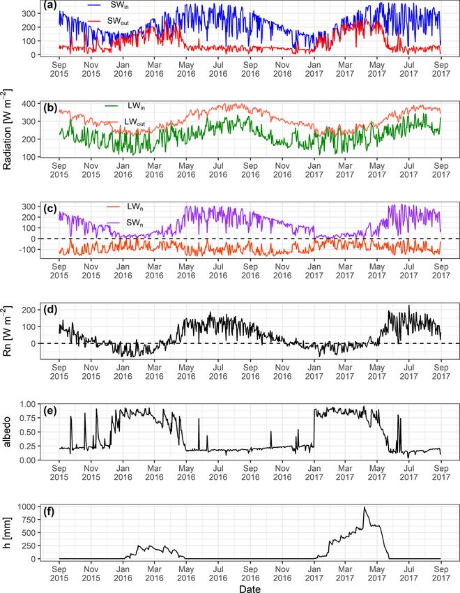
2274                             J. M. Wani et al.: The surface energy balance in a cold and arid permafrost environment

of the glaciers than previously known (Bhutiyani, 1999; Im-       (Rastogi and Narayan, 1999; Wünnemann et al., 2008) and
merzeel et al., 2015; Thayyen, 2020).                             the Changla region (Ali et al., 2018).
   The sensitivity of mountain permafrost to climate change          The SEB characteristics of different permafrost regions
(Haeberli et al., 2010) leads to changes in permafrost condi-     have been studied in e.g. the North American Arctic (Eugster
tions such as an increase in active layer thickness that even-    et al., 2000; Lynch et al., 1999; Ohmura, 1982, 1984), Euro-
tually may affect the ground stability (Gruber and Haeberli,      pean Arctic (Lloyd et al., 2001; Westermann et al., 2009),
2007; Salzmann et al., 2007), trigger debris flows and rock-      Tibetan Plateau (Gu et al., 2015; Hu et al., 2019; Yao et al.,
falls (Gruber et al., 2004; Gruber and Haeberli, 2007; Harris     2008, 2011, 2020), European Alps (Mittaz et al., 2000) and
et al., 2001), hydrological changes (Woo et al., 2008), run-      Siberia (Boike et al., 2008; Kodama et al., 2007; Langer et
off patterns (Gao et al., 2018; Wang et al., 2017), water qual-   al., 2011a, b). However, SEB studies of IHR are limited to,
ity (Roberts et al., 2017), greenhouse gas emissions (Mu et       for example, the energy balance studies on glaciers by Azam
al., 2018), alpine ecosystem changes (Wang et al., 2006), and     et al. (2014) and Singh et al. (2020). Besides its effect on
unique construction requirements to negate the effects caused     heat transport into the subsurface, the SEB may also have a
by ground-ice degradation (Bommer et al., 2010). These im-        significant influence on regional and local climate (Eugster
pacts strongly affect mountain communities and indicate the       et al., 2000). During summer months, permafrost creates a
relevance of mountain permafrost on human livelihoods.            heat sink which reduces the surface temperature and there-
   The energy balance at the earth’s surface drives the spatio-   fore reduces heat transfer to the atmosphere (Eugster et al.,
temporal variability in ground temperature (Oke, 2002; Sell-      2000). This highlights that the knowledge of frozen ground
ers, 1965; Westermann et al., 2009). It is linked to the at-      and associated energy regimes is a critical knowledge gap
mospheric boundary layer and location-dependent transfer          in our understanding of the Himalayan cryospheric systems,
mechanisms between land and the overlying atmosphere              especially in the UIB.
(Endrizzi, 2007; Martin and Lejeune, 1998; McBean and                The goal of this paper is to improve the understanding of
Miyake, 1972). The surface energy balance (SEB) in cold           permafrost in cold and arid UIB areas and to advance our
regions additionally depends on the seasonal snow cover,          ability to analyse and simulate its characteristics. This can
vegetation and moisture availability in the soil (Lunardini,      guide the application of available permafrost models in the
1981), and (semi-)arid areas exhibit their typical characteris-   Ladakh region, which are calibrated (Boeckli et al., 2012) or
tics (Xia, 2010).                                                 validated (Cao et al., 2019; Fiddes et al., 2015) elsewhere.
   The role of permafrost is a key unknown variable in the        Furthermore, it can help to interpret differences in surface
Himalayas, especially in headwater catchments of the Indus        offsets (difference between the mean annual ground surface
basin. A recent study has signalled significant permafrost oc-    and mean annual air temperatures) observed in Ladakh (Wani
currence in the cold and arid areas of the upper Indus basin      et al., 2020) and other permafrost areas (Boeckli et al., 2012;
(UIB) covering Ladakh (Wani et al., 2020). Large-scale as-        Hasler et al., 2015; PERMOS, 2019). Our working hypoth-
sessment in the Hindu Kush Himalayan (HKH) region sug-            esis is that the surface offset for particular terrain types in
gests that the permafrost area covers up to 1 million km2 ,       the UIB differs from what is known from other areas, driven
which roughly translate into 14 times the area of glacier         by aridity and high elevation. We aim to improve the un-
cover of the region (Gruber et al., 2017). Except for Bhutan,     derstanding of the SEB and its relationship with the ground
the expected permafrost areas in all other countries in the       temperature by working on three objectives: (1) quantifying
HKH region is larger than the glacier area (cf. Table 1, Gru-     the SEB at South Pullu as an example for permafrost areas
ber et al., 2017).                                                in the UIB; (2) understanding the pronounced seasonal and
   The mapping of rock glaciers using remote sensing sug-         inter-annual variation in snowpack and near-surface ground
gested that the discontinuous permafrost in the HKH region        temperature (GST) as these are intermediate phenomena be-
can be found from 3500 m a.s.l. in northern Afghanistan to        tween the SEB and permafrost; and (3) understanding key
5500 m a.s.l. on the Tibetan Plateau (Schmid et al., 2015). In    differences with other permafrost areas that have SEB obser-
the Indian Himalayan Region (IHR), recent studies show that       vations.
the discontinuous permafrost can be found between 3000 and
5500 m a.s.l. (Allen et al., 2016; Baral et al., 2019; Pandey,
2019).                                                            2     Study area and data
   The cold and arid region of Ladakh has a reported sporadic
occurrence of permafrost and associated landforms (Gruber         2.1    Study area
et al., 2017; Wani et al., 2020) with sorted patterned ground
and other periglacial landforms such as ice-cored moraines.       The present study is carried out at South Pullu (34.25◦ N,
Field observations suggest that ground-ice melt may also be       77.62◦ E; 4727 m a.s.l.) in the upper Ganglass catchment
a critical water source in dry summer years in the cold and       (34.25 to 34.30◦ N and 77.50 to 77.65◦ E), Leh, Ladakh
arid regions of Ladakh (Thayyen, 2015). Previous studies of       (Fig. 1). Ladakh is a union territory of India and has a
permafrost in the Ladakh region are from the Tso Kar basin        unique climate, hydrology and landforms. Leh is the dis-

The Cryosphere, 15, 2273–2293, 2021                                                   https://doi.org/10.5194/tc-15-2273-2021
The surface energy balance in a cold and arid permafrost environment, Ladakh, Himalayas, India - The Cryosphere
J. M. Wani et al.: The surface energy balance in a cold and arid permafrost environment                                               2275

Figure 1. Location of the study site in the upper Ganglass catchment. (Base image sources for the right panel: © Esri, DigitalGlobe, GeoEye,
Earthstar Geographic’s, CNES/Airbus DS, USDA, USGS, AEX, Getmapping, Aerogrid, IGN, IGP, swisstopo and the GIS user community).
Please note that the above figure contains disputed territories.

trict headquarter where long-term climate data are available            Sutron automatic weather station from 1 September 2015 to
(Bhutiyani et al., 2007). Long-term mean precipitation of               31 August 2017. The study years 1 September 2015 to 31 Au-
Leh (1980–2017, 3526 m a.s.l.) is 115 mm (Lone et al., 2019;            gust 2016 and 1 September 2016 to 31 August 2017 hereafter
Thayyen et al., 2013), and the daily minimum and maximum                in the text will be designated as 2015–2016 and 2016–2017,
temperatures during the period (2010 to 2012) range between             respectively. The variables measured include air tempera-
−23.4 and 33.8 ◦ C (Thayyen and Dimri, 2014). The spatial               ture, relative humidity, wind speed and direction, incoming
area of the catchment is 15.4 km2 and extends from 4700 m               and outgoing short-wave and long-wave radiation, and snow
to 5700 m a.s.l. A small cirque glacier called Phuche glacier           depth (Table 1). The snow depth is measured using a Camp-
with an area of 0.62 km2 occupies the higher elevations of              bell SR50 sonic ranging sensor with a nominal accuracy of
the catchment, where a single stream originates and flows               ±1 cm (Table 1). To reduce the noise of the measured snow
through the valley of the catchment. This stream flows inter-           depth, a 6 h moving average is applied. Near-surface ground
mittently with a maximum mean daily flow of 3.57 m3 s−1                 temperature (GST) is measured at a depth of 0.1 m near the
(wet years) and 0.4 m3 s−1 (dry years) from May to October.             AWS using a miniature temperature data logger (MTD) man-
   The catchment is part of the main Indus River basin                  ufactured by GeoPrecision GmbH, Germany. GST data were
and belongs to the geological unit of the Ladakh batholith              available only from 1 September 2016 to 31 August 2017
(Thakur, 1981). The study catchment also consists of steep              and are used for model evaluation only. All the four solar
mountain slopes with the valley bottom filled with glacio-              radiation components, i.e. incoming short-wave (SWin ), out-
fluvial deposits. Other sporadic landforms found in the catch-          going short-wave (SWout ), incoming long-wave (LWin ) and
ment include patterned ground, boulder fields, peatlands,               outgoing long-wave (LWout ) radiation, were measured. Be-
high-elevation wetlands and a small lake. Many of these                 fore using these data in the SEB calculations, necessary cor-
landforms point towards intense frost action in the area.               rections were applied (Nicholson et al., 2013; Oerlemans and
                                                                        Klok, 2002): (a) all the values of SWin < 5 W m−2 are set to
2.2   Meteorological data used                                          zero, and (b) when SWout > SWin (3 % of data under study),
                                                                        it indicates that the upward-looking sensor was covered with
                                                                        snow (Oerlemans and Klok, 2002). The SWout can be higher
The automatic weather station (AWS) in the catchment is lo-
                                                                        than SWin at high-elevation sites such as this one due to
cated at an elevation of 4727 m a.s.l. at South Pullu (Fig. 1).
                                                                        high solar zenith angle during the morning and evening hours
It is located in a wide south-east-oriented deglaciated val-
                                                                        (Nicholson et al., 2013). In such cases, SWin was corrected
ley. The site has a local slope angle of 15◦ , and the soil is
                                                                        by SWout divided by the accumulated albedo, calculated by
sparsely vegetated. Weather data have been collected by a

https://doi.org/10.5194/tc-15-2273-2021                                                        The Cryosphere, 15, 2273–2293, 2021
The surface energy balance in a cold and arid permafrost environment, Ladakh, Himalayas, India - The Cryosphere
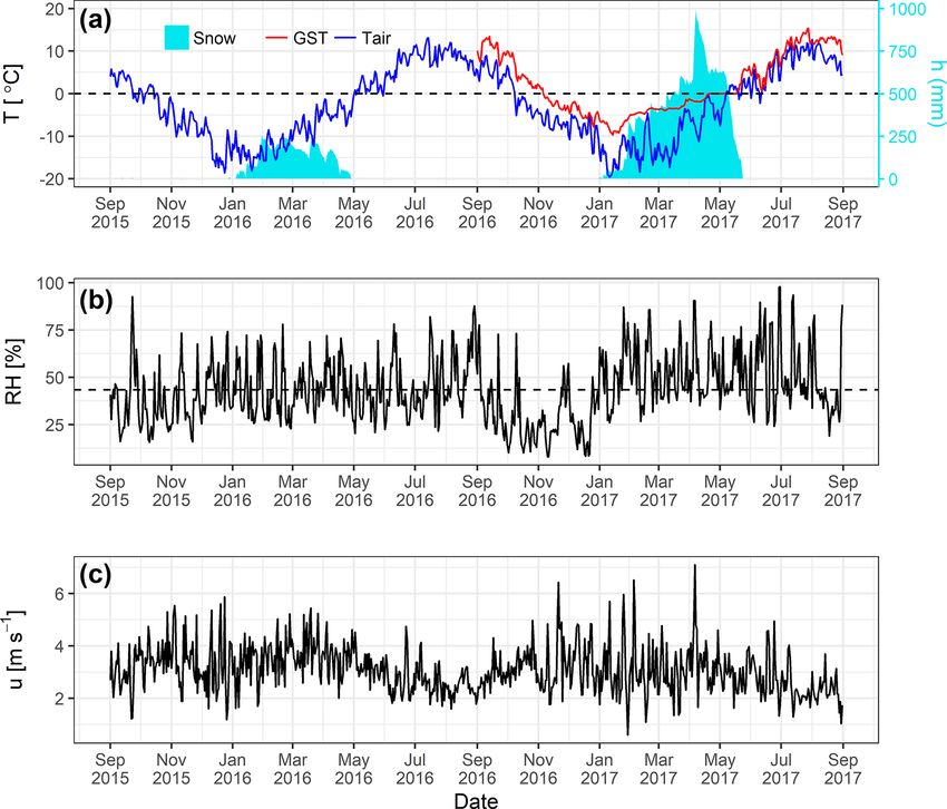
2276                               J. M. Wani et al.: The surface energy balance in a cold and arid permafrost environment

Table 1. Technical parameters of different sensors at South Pullu (4727 m a.s.l.) in the upper Ganglass catchment, Leh. (MF: model forcing,
ME: model evaluation).

       Variable                          Units        Sensor                                    Stated accuracy    Height (m)    Use
       Air temperature                   (◦ C)        Rotronics-5600-0316-1                     ±0.2 ◦ C                   2.2   MF
       Relative humidity                 (%)          Rotronics-5600-0316-1                     ±1.5 %                     2.2   MF
       Wind speed                        (m s−1 )     RM Young 05103-45                         ±0.3 m s−1                  10   MF
       Wind direction                    (◦ )         RM Young 05103-45                         ±0.3◦                       10   MF
       Incoming short-wave radiation     (W m−2 )     Kipp and Zonen (CMP6) (285 to             ±10 %                      4.6   MF
                                                      2800 nm)
       Outgoing short-wave radiation     (W m−2 )     Kipp and Zonen (CMP6) (285 to             ±10 %                      4.6   MF
                                                      2800 nm)
       Incoming long-wave radiation      (W m−2 )     Kipp and Zonen (CGR3) (4500 to            ±10 %                      4.3   MF
                                                      42 000 nm)
       Outgoing long-wave radiation      (W m−2 )     Kipp and Zonen (CGR3) (4500 to            ±10 %                      4.3   ME
                                                      42 000 nm)
       Snow depth                        (m)          Campbell SR-50                            ±1 cm                    3.44    ME
       Data logger                       –            Sutron 9210-0000-2B                       –                           –    –
       Near-surface ground temperature   (◦ C)        PT1000 in stainless steel cap (by Geo-    ±0.1 ◦ C                 −0.1    ME
                                                      Precision GmbH, Germany)

the ratio of measured SWout and measured SWin for a 24 h                      and if Tw >=1 (rain), Tw is estimated by solving the psy-
period (van den Broeke et al., 2004).                                         chrometric formula implicitly: e = E (Tw )−γ (Ta −Tw ),
                                                                              where Ta is the air temperature, e (hPa) is the vapour
                                                                              pressure in the air, E (hPa) is the saturation vapour pres-
3     Methods                                                                 sure, and γ (hPa K−1 ) is the psychrometric constant de-
                                                                              pending on air pressure.
3.1    Estimation of precipitation from snow height
                                                                          3. For the estimation of density, the fresh snow density
In high-elevation and remote sites, the measurement of snow-                 (ρ) is estimated based on air temperature (Ta ) and wind
fall is a difficult task with an undercatch of 20 %–50 %                     speed measured at 10 m height (u10 ) as follows (Jordan
(Rasmussen et al., 2012; Yang et al., 1999). At the South                    et al., 1999):
Pullu station, daily precipitation including snow was mea-
sured using a non-recording rain gauge. In this high-elevation                ρ = 500 · [1 − 0.951 · exp(−1.4
area, an undercatch of 23 % of snowfall was reported earlier                    · (278.15 − Ta )−1.15 − 0.008u1.7                      (1)
                                                                                                              10 )]
(Thayyen et al., 2015). In this study, the total precipitation
was recorded at daily temporal resolution, whereas the other                  for 260.15 < Ta ≤ 275.65 K.
meteorological forcings including SR50 snow depth were
recorded at hourly time steps. Therefore, to match the tempo-                 ρ = 500 · [1 − 0.904 · exp(−0.008u1.7                    (2)
                                                                                                                10 )]
ral resolution of precipitation data with the other meteorolog-
ical forcing data, we adopted the method proposed by Mair                     for Ta ≤ 260.15 K.
et al. (2016), called Estimating SOlid and Liquid Precipita-
tion (ESOLIP). This method makes use of snow depth and                    4. To estimate the SWE (SWE = h · ρ) of single snowfall
meteorological observations to estimate the sub-daily solid                  events using snow depth (h) measurements, an identifi-
precipitation in terms of snow water equivalent (SWE). In                    cation of the snow height increments of the single snow-
ESOLIP, we considered daily liquid precipitation only. The                   fall events and an accurate estimate of the snow density
ESOLIP method consists of the following steps:                               are necessary.

    1. Precipitation readings related to simplified relative hu-        3.2   Modelling of surface energy balance
       midity (RH) and global short-wave radiation criteria
       (e.g. RH > 50 % and SWin < 400 W m−2 ) are filtered.             In this study, the open-source model GEOtop version 2.0
                                                                        (hereafter GEOtop) (Endrizzi et al., 2014; Rigon et al., 2006)
    2. For precipitation type determination, wet bulb tempera-          was used for the modelling of point surface energy balance,
       ture (Tw ) is used to differentiate between rain and snow,       including the evolution of the snow depth and the transfer
       i.e. rainfall is assumed for Tw < 1 (SWE estimation),            of heat and water in snow and soil. GEOtop represents the

The Cryosphere, 15, 2273–2293, 2021                                                          https://doi.org/10.5194/tc-15-2273-2021
The surface energy balance in a cold and arid permafrost environment, Ladakh, Himalayas, India - The Cryosphere
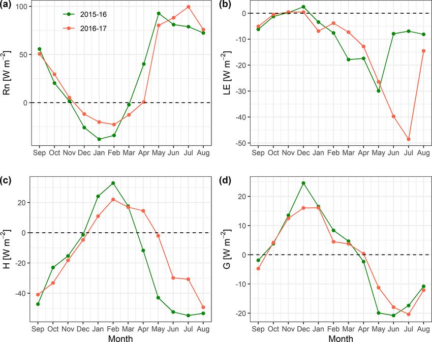
J. M. Wani et al.: The surface energy balance in a cold and arid permafrost environment                                        2277

combined ground heat and water balance, as well as the ex-         where Ts , the temperature of the surface, is unknown, SWn
change in energy with the atmosphere by taking into con-           is the net short-wave radiation, LWn is the net long-wave ra-
sideration the radiative and turbulent heat fluxes. The model      diation, and Fsurf is a function of Ts . Other terms in Eq. (4)
has a multi-layer snowpack and solves the energy and water         which are a function of Ts include LWn , H and LE. In addi-
balance of the snow cover and soil including the highly non-       tion, LE depends also on the soil moisture at the surface (θw ),
linear interactions between the water and energy balance dur-      linking the SEB and water balance equations. The equations
ing soil freezing and thawing (Dall’Amico et al., 2011a). It       and the key elements of GEOtop are explained in Endrizzi et
can be applied in complex terrain which makes it possible to       al. (2014); here, only a brief description of the equations that
account for topographical and other environmental variabil-        are of interest in this study is given. LWout is estimated using
ity (Fiddes et al., 2015; Gubler et al., 2013).                    the Stefan–Boltzmann law:
   Previous studies have successfully applied GEOtop in
mountain regions e.g. simulating snow depth (Endrizzi et al.,
2014), snow cover mapping (Dall’Amico et al., 2011b, 2018;         LWout = ∈s σ Ts4 ,                                            (5)
Engel et al., 2017; Zanotti et al., 2004), ecohydrological pro-
cesses (Bertoldi et al., 2010; Chiesa et al., 2014), modelling
                                                                   where ∈s is the surface emissivity, and σ is the Stefan–
of ground temperatures in complex topography (Bertoldi et
                                                                   Boltzmann constant (5.67 × 10⁻⁸ W m−2 K−4 ).
al., 2010; Endrizzi et al., 2014; Fiddes and Gruber, 2012;
                                                                      The turbulent fluxes (H and LE) are driven by the gra-
Gubler et al., 2013), water and energy fluxes (Hingerl et al.,
                                                                   dients of temperature and specific humidity between the air
2016; Rigon et al., 2006; Soltani et al., 2019), evapotran-
                                                                   and the surface and due to turbulence caused by winds as the
spiration (Mauder et al., 2018), and permafrost distribution
                                                                   primary transfer mechanism in the boundary layer (Endrizzi,
(Fiddes et al., 2015).
                                                                   2007). GEOtop estimates the turbulent heat fluxes using the
   Generally, the surface energy balance (SEB) (Eq. 3) is
                                                                   flux-gradient relationship (Brutsaert, 1975; Garratt, 1994) as
written as a combination of net radiation (Rn ), sensible (H )
                                                                   follows:
and latent heat (LE) flux, heat conduction into the ground or
to the snow (G), and it must balance at all times (Oke, 2002):
                                                                                Ta − Ts
Rn + H + LE + G − Fsurf = 0,                                (3)    H = ρa cp ws          ,                                       (6)
                                                                                   ra
where Fsurf is the resulting latent heat flux in the snow-                               Qa − αY P Q∗s
                                                                   LE = βY P Le ρa cp ws               ,                         (7)
pack due to melting or freezing. We use the sign conven-                                      ra
tion that energy fluxes towards the surface are positive and
fluxes away from the surface are negative (Mölg, 2004). Dur-
ing the summertime, when conditions for snow melting are           where ρa is the air density (kg m−3 ), ws is the wind
prevailing at the ground surface, Fsurf is negative (loss from     speed (m s−1 ), cp the specific heat at constant pressure
the system) as a result of energy available for melting snow       (J kg−1 K−1 ), Le the specific heat of vaporization (J kg−1 ),
and warming the ground under snow-free conditions. Posi-           Qa and Q∗s are the specific humidity of the air (kg kg−1 ) and
tive Fsurf (gain to the system) during summertime is the en-       saturated specific humidity at the surface (kg kg−1 ), respec-
ergy released to refreeze the water and represents the freezing    tively, βY P and αY P are the coefficients that take into ac-
flux.                                                              count the soil resistance to evaporation and only depend on
   In cold regions, the SEB is a complex function of so-           the liquid water pressure close to the soil surface, and ra is the
lar radiation, seasonal snow cover, vegetation, near-surface       aerodynamic resistance (–). The aerodynamic resistance is
moisture content and atmospheric temperature (Lunardini,           obtained by applying the Monin–Obukhov similarity theory
1981). Based on the available in situ data, the calculation        (Monin and Obukhov, 1954), which requires that values of
of SEB components like H , LE and G is difficult. For ex-          wind speed, air temperature and specific humidity are avail-
ample, in the calculation of turbulent heat fluxes (H and          able at least at two different heights above the surface, but
LE), the wind speed and temperature measurements near the          the values of these variables are generally measured at a stan-
ground surface are required at two heights, which are gen-         dard height above the surface and can be used for the ground
erally not available. Therefore, the parameterization method,      surface with the following assumptions: (a) the air tempera-
like the bulk aerodynamic method, is used, which is valid          ture is equal to the ground surface temperature; however, this
under statically neutral conditions in the surface layer (Stull,   assumption leads to the boundary condition’s non-linearity,
1988). Hence, the application of a tested model like GEOtop        (b) the specific humidity is equal to αY P Q∗s , and (c) wind
is a good alternative for the estimation of these fluxes. In       speed is equal to zero.
GEOtop, the general SEB equation (Eq. 3) is linked with the           The coefficients βY P and αY P (Eqs. 8 and 9) are calculated
water balance and is written as follows:                           according to the parameterization of Ye and Pielke (1993)
                                                                   which considers evaporation as the sum of the proper evapo-
Fsurf (Ts ) = SWn + LWn (Ts ) + H (Ts ) + LE (Ts , θw ) ,   (4)    ration from the surface and diffusion of water vapour in soil

https://doi.org/10.5194/tc-15-2273-2021                                                  The Cryosphere, 15, 2273–2293, 2021
The surface energy balance in a cold and arid permafrost environment, Ladakh, Himalayas, India - The Cryosphere
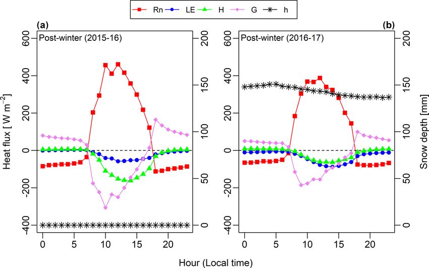
2278                              J. M. Wani et al.: The surface energy balance in a cold and arid permafrost environment

pores at greater depths:                                             et al. (2003). Fresh snow density is computed using the Jor-
                                                                   dan et al. (1999) formula, which is based on air temperature
                   χp (g) − θg                                       and wind speed. More details about the snow metamorphism
βY P = χp (g) −      χ (1)−θ ra
                                    ,                         (8)
                 1 + χpp (g)−θ(1)                                    compaction rates and the snow discretization in GEOtop can
                               g rd
                                                                   be found in Appendix D2 and D3 of Endrizzi et al. (2014).
                                                  sat
                                                 q(Ts1)
          1          χp (1) − θ(1) ra
αY P =         θg +                        h
                          χ (1)−θ(1) ra r s(θ1 ) q sat
                                                        ,    (9)    3.2.2   Model setup and forcings
        βY P        1+ p                 d         (Tg)
                          χp (g)−θg rd
                                                                     The 1D GEOtop simulation was carried out at South Pullu
where q sat is the specific humidity in saturated condition, the     (Fig. 1). The soil column is 10 m deep and is discretized into
subscripts “g” and 1 refer to the ground surface and a thin          19 layers, with thickness increasing from the surface to the
layer next to the ground surface, respectively, θ is the volu-       deeper layers. The top eight layers close to the ground sur-
metric water content of the soil, χp is the volumetric fraction      face were resolved with thicknesses ranging from 0.1 to 1 m
of soil pores, hs is the relative humidity in the pores, Tg is the   because of the higher temperature and water pressure gradi-
temperature at the ground surface, and rd is the soil resistance     ents near the surface, while the lowest layer is 4.0 m thick.
to water vapour diffusion.                                           The snowpack is discretized in 10 layers which are finer at
                                                                     the interfaces with the atmosphere and soil.
3.2.1   The heat equation and snow depth
                                                                        The model was initialized with a uniform soil tempera-
Equation (10) represents the energy balance in a soil volume         ture of −0.5 ◦ C and spun up by repeatedly modelling the soil
subject to phase change in GEOtop (Endrizzi et al., 2014):           temperature down to 1 m (2 years · 25 times) and then using
                                                                     the modelled soil temperatures as an initial condition to re-
∂U ph                                                                peatedly simulate soil temperature down to 10 m (2 years · 25
      + ∇G + Sen − ρw [Lf + cw (T − Tref )] Sw = 0,          (10)    times) (cf., Fiddes et al., 2015; Gubler et al., 2013; Pogliotti,
 ∂t
                                                                     2011). Prior tests showed that the minimum number of rep-
where U ph is the volumetric internal energy of soil (J m−3 )        etitions required to bring the soil column to equilibrium was
subject to phase change, t (s) is time, G is the heat conduc-        25 (Fig. S1). The values of all the input parameters used in
tion flux (W m−2 ), Sen is the energy sink term (W m−3 ), Sw         the study are given in Tables A1 to A4 in the Supplement.
is the mass sink term (s−1 ), Lf (J kg−1 ) is the latent heat of        The input meteorological data required for running the 1D
fusion, ρw is the density of liquid water in soil (kg m−3 ), cw      GEOtop model include time series of precipitation, air tem-
is the specific thermal capacity of water (J kg−1 K−1 ), T (◦ C)     perature, relative humidity, wind speed, wind direction (WD)
is the soil temperature, and Tref (◦ C) is the reference tempera-    and solar radiation components and the description of the site
ture at which the internal energy is calculated. If G is written     (slope angle, elevation, aspect and sky view factor) for the
according to Fourier’s law, Eq. (10) becomes                         simulation point. The model was run at an hourly time step
                                                                     corresponding to the measurement time step of the meteoro-
∂U ph                                                                logical data.
      + ∇(λT ∇T ) + Sen − ρw [Lf + cw (T − Tref )] Sw = 0,
 ∂t
                                                       (11)          3.2.3   Model performance evaluation

where λT is the thermal conductivity (W m−1 K−1 ), which is          While the accuracy of simulated energy fluxes cannot be
a non-linear function of temperature because the proportion          quantified, the quality of GEOtop simulations is evaluated
of liquid water and ice contents depends on temperature. For         based on snow depth, GST and LWout . These variables were
the calculation of λT , GEOtop uses the method proposed by           chosen because they have not been used to drive the model,
Cosenza et al. (2003). A detailed description of the heat con-       and they represent different physical processes affected by
duction equation used in GEOtop can be found in Endrizzi et          surface energy balance. The melt-out date of the snow depth
al. (2014).                                                          is hereby a good indicator showing how good the surface
   The snow cover buffers the energy exchange between the            mass and energy balance is simulated, whereas GST is the re-
soil and atmosphere and critically influences the soil ther-         sult of all the processes occurring at the ground surface such
mal regime. GEOtop includes a multi-layer, energy-based,             as radiation, turbulence, and latent and sensible heat fluxes
Eulerian snow modelling approach with similar equations to           (Gubler, 2013). LWout is governed by the temperature and
the ones used for the soil matrix (Endrizzi et al., 2014). The       emissivity at the surface, and Eq. (3) is solved in terms of the
discretization of snow in GEOtop is carried out in such a            surface temperature. Therefore, LWout is used as a proxy for
way that the thermal gradients inside the snowpack are de-           the evaluation of the SEB.
scribed accurately. The effective thermal conductivity at the           Model performance is evaluated based on the measured
interface between snow and ground is calculated similarly as         and the simulated time series. Typically, a variety of sta-
between different soil layers using the method of Cosenza            tistical measures are used to assess the model performance

The Cryosphere, 15, 2273–2293, 2021                                                      https://doi.org/10.5194/tc-15-2273-2021
The surface energy balance in a cold and arid permafrost environment, Ladakh, Himalayas, India - The Cryosphere
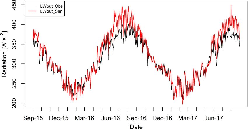
J. M. Wani et al.: The surface energy balance in a cold and arid permafrost environment                                            2279

Figure 2. Comparison of hourly observed and GEOtop-simulated
snow depth at South Pullu (4727 m a.s.l.) from 1 September 2015 to    Figure 3. Comparison of daily mean observed (GST_obs; ◦ C) and
31 August 2017. The black line denotes the snow depth measured        GEOtop-simulated near-surface ground temperature (GST_sim;
                                                                      ◦ C) at South Pullu (4727 m a.s.l.) from 1 September 2016 to 31 Au-
in the field by the SR50 sensor. The red (Snow depth_ESOLIP)
and green (Snow depth_field) lines in the plot indicate the GEOtop-   gust 2017.
simulated snow depth based on ESOLIP-estimated precipitation and
precipitation measured in the field, respectively.
                                                                      measured in the field (Fig. 2). ESOLIP is the superior ap-
                                                                      proach for precipitation estimation when snow depth and
because no single measure encapsulates all aspects of in-             necessary meteorological measurements are available.
terest. In this study, R 2 , mean bias difference (MBD) and              Figure 2 shows the comparison of hourly observed and
the root mean square difference (RMSD), mean bias (MB)                GEOtop-simulated snow depth at South Pullu (4727 m a.s.l.)
and root mean square error (RMSE), and Nash–Sutcliffe effi-           from 1 September 2015 to 31 August 2017. The black line
ciency coefficient (NSE; Nash and Sutcliffe, 1970) were used          denotes the snow depth measured in the field by the SR50
(Eqs. S1 to S6).                                                      sensor. The red (Snow depth_ESOLIP) and green (Snow
                                                                      depth_field) lines in the plot indicate the GEOtop-simulated
                                                                      snow depth based on ESOLIP-estimated precipitation and
4     Results                                                         precipitation measured in the field, respectively.

4.1     Model evaluation                                              4.1.2   Evaluation of near-surface ground temperatures
                                                                              (GST)
In this section, the capability of GEOtop to reproduce snow
depth, GST and LWout based on standard model parameters               GST is simulated (GST_sim) on an hourly basis and com-
obtained from the literature (Tables 2 and 3; Gubler et al.,          pared with the observed values (GST_obs) near the AWS,
2013) was evaluated, i.e. model results were not improved             available from 1 September 2016 to 31 August 2017 (Fig. 3).
by trial and error.                                                   The results show a reasonably good linear agreement be-
                                                                      tween the simulated and observed GSTs (Fig. S3; R 2 = 0.97,
4.1.1    Evaluation of snowpack                                       MB = −0.11 ◦ C, RMSE = 1.63 ◦ C, NSE = 0.95, instrument
                                                                      error = ±0.1◦ ). The model estimated the dampening of soil
Snow depth variations simulated by GEOtop are compared                temperature fluctuations by the snowpack and the zero-
with observations from 1 September 2015 to 31 August 2017             curtain period at the end of the melt-out of the snowpack
(Fig. 2). The model captures the peaks and start and melt-            reasonably well.
out dates of the snowpack, as well as overall fluctuations
(Fig. S2; R 2 = 0.98, RMSE = 59.5 mm, MB = 16.7 mm,                   4.1.3   Evaluation of outgoing long-wave radiation
NSE = 0.91, instrument error = ±10 mm). The maximum
simulated snow height (h) was 1219 mm in comparison to the            Modelled LWout is evaluated with the observed measure-
1020 mm measured in the field. In the low snow year (2015–            ments, and a comparison of daily mean observed and sim-
2016), the maximum simulated h was 326 mm in comparison               ulated LWout is shown in Fig. 4. The daily mean LWout
to 280 mm measured in the field. During the melting period            matches very well with the observed data except during
of the low and high snow years, the snow depth was slightly           summer months when the simulated LWout was slightly
underestimated. However, during the accumulation period of            overestimated compared to the observed values. The hourly
high snow year (2016–2017), h was rather overestimated by             LWout shows a good linear relationship (Fig. S4; R 2 = 0.93,
the model.                                                            NSE = 0.73), but the GEOtop slightly overestimates the
   The performance of the ESOLIP-estimated precipitation              LWout (MBD = 3 %) with an RMSD value of 10 % (instru-
was evaluated against a control run with precipitation data           ment error = ±10 %).

https://doi.org/10.5194/tc-15-2273-2021                                                      The Cryosphere, 15, 2273–2293, 2021
The surface energy balance in a cold and arid permafrost environment, Ladakh, Himalayas, India - The Cryosphere
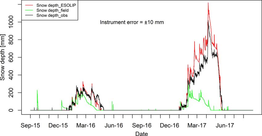
2280                                J. M. Wani et al.: The surface energy balance in a cold and arid permafrost environment

                                                                        2-year study period, sub-zero mean monthly temperature pre-
                                                                        vailed for 7 months from October to April in both years.
                                                                        The mean monthly Ta during pre-winter months (Septem-
                                                                        ber to December) of 2015–2016 and 2016–2017 was −4.6
                                                                        and −2.7 ◦ C, respectively. During the core winter months
                                                                        (January to February) of 2015–2016 and 2016–2017, the re-
                                                                        spective mean monthly Ta was −13.1 and −13.7 ◦ C, and, for
                                                                        post-winter months (March and April), mean monthly Ta was
                                                                        −5.8 and −8 ◦ C, respectively. For summer months (May to
                                                                        August), the respective mean monthly Ta was 6.6 and 5.5 ◦ C.
                                                                        A sudden change in the mean monthly Ta characterizes the
Figure 4. Comparison of daily mean observed (LWout _obs) and            onset of a new season, and the most evident inter-season
GEOtop-simulated (LWout _sim) outgoing long-wave radiation at           change was found between the winter and summer with a
South Pullu (4727 m a.s.l.) from 1 September 2015 to 31 Au-             difference of about 16 ◦ C for both years.
gust 2017. The instrument error for the Kipp and Zonen (CGR3)              The mean daily GST recorded by the logger near the AWS
(4500 to 42 000 nm) radiometer is ±10 %.                                (1 September 2016 to 31 August 2017) is plotted along with
                                                                        air temperature (Fig. 5a). The mean daily GST ranges from
Table 2. Range of observed daily mean radiation components              −9.7 to 15.4 ◦ C with a mean annual GST of 2.1 ◦ C. The GST
(SWin , SWout , LWin and LWout , SWn , LWn ), surface albedo (α),       followed the pattern of air temperature but damped during
net short-wave and long-wave radiation (SWn and LWn ), air tem-         winter due to the insulating effect of the snow cover. GST
perature (Ta ), wind speed (u), relative humidity (RH), precipitation   was generally higher than Ta except for a short period dur-
(P ), and snow depth (h) for the study period (1 September 2015 to      ing snowmelt. The snow depth shown in Fig. 5a is further
31 August 2017) at South Pullu (4727 m a.s.l.).                         described in Sect. 4.3.
                                                                           Mean relative humidity (RH) was equal to 43 % during
      Variable   Units           Min.         Max.        Mean          the study period (Fig. 5b). The daily average wind speed
      SWin       W m−2           24.1        377.8        210.4         (u) ranges between 0.6 (29 January 2017) and 7.1 m s−1
      SWout      W m−2        (−) 2.4    (−) 262.6     (−) 83.4         (6 April 2017) with a mean wind speed of 3.1 m s−1 (Fig. 5c).
      α          –               0.04         0.95         0.43         The instantaneous hourly u was plotted as a function of wind
      LWin       W m−2          109.0        344.7        220.4         direction (WD) (Fig. S5) for the study period and showed
      LWout      W m−2      (−) 211.3    (−) 400.0    (−) 308.0         a persistent dominance of katabatic and anabatic winds at
      SWn        W m−2            2.5        318.7        127.0         the study site, which is typical of a mountain environment.
      LWn        W m−2          −163          17.1       −87.6          The daily average WD during the study period was south-
      Ta         ◦C            −19.5          13.1        −2.5          east (148◦ ).
      u          m s−1            0.6          7.1          3.1            The daily measured annual total precipitation at the study
      RH         %                  8           98         43.3         site equals 97.8 and 153.4 mm w.e. during the years 2015–
      P          mm w.e.            0         24.6            3         2016 and 2016–2017, respectively. After adding 23 % un-
      h          mm                 0          991            –         dercatch (Thayyen et al., 2015) to the total snow mea-
                                                                        surements, the total precipitation amount equals 120.3 and
                                                                        190.6 mm w.e. for the years 2015–2016 and 2016–2017,
   Based on the evaluation of LWout , the GEOtop can sim-               respectively. During the study period, the observed high-
ulate the surface temperature at the point scale; therefore,            est single-day precipitation was 20 mm w.e. recorded on
we believe that it can reasonably calculate the different SEB           23 September 2015, and the total number of precipitation
components.                                                             days was limited to 63. The snowfall occurs mostly during
                                                                        the winter period (December to March), with some years wit-
4.2     Meteorological characteristics                                  nessing extended intermittent snowfall till mid-June, as expe-
                                                                        rienced in this study during the year 2016–2017.
The range of the meteorological variables measured at the                  The precipitation estimated by the ESOLIP approach at
South Pullu (4727 m a.s.l.) study site is given in Table 2              the study site equals 92.2 and 292.5 mm w.e. during the years
to provide an overview of the prevailing weather condi-                 2015–2016 and 2016–2017, respectively. The comparison
tions in the study region. The daily mean air temperature               between observed precipitation (mm w.e.) and the one esti-
(Ta ) throughout the study period varies between −19.5 and              mated by the ESOLIP approach is given in (Table S1). In
13.1 ◦ C with a mean annual average temperature (MAAT) of               Table S1, the difference between the observed precipitation
−2.5 ◦ C (Fig. 5a). Ta shows significant seasonal variations,           (mm w.e.) and the one estimated by the ESOLIP approach is
and measured hourly temperatures at the study site range be-            mainly due to the undercatch of winter snow recorded by the
tween −23.7 ◦ C in January and 18.1 ◦ C in July. During the             ordinary rain gauge.

The Cryosphere, 15, 2273–2293, 2021                                                        https://doi.org/10.5194/tc-15-2273-2021
J. M. Wani et al.: The surface energy balance in a cold and arid permafrost environment                                                2281

Figure 5. Daily mean values of observed (a) air temperature (blue) and 1-year GST (red) (T ; ◦ C) with snow depth (mm) on the secondary
axis, (b) relative humidity (RH; %) with a dashed line as mean RH, and (c) wind speed (u; m s−1 ) at South Pullu (4727 m a.s.l.) in the upper
Ganglass catchment, Leh, from 1 September 2015 to 31 August 2017.

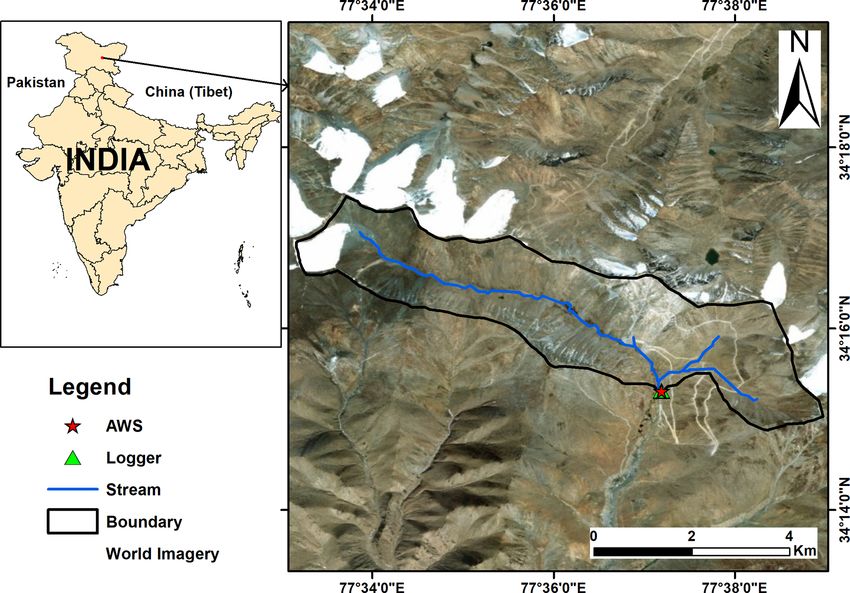
4.3   Observed radiation components and snow depth                       During both years, Rn was high in summer and autumn but
                                                                         low in winter and spring. From January to early April (2015–
The observed daily mean variability in different components              2016) and January to early May (2016–2017), when the sur-
of radiation, albedo and snow depth from 1 September 2015                face was covered with seasonal snow, Rn rapidly declined
to 31 August 2017 at South Pullu (4727 m a.s.l.) is shown in             to low values or even became negative (Fig. 6d). Daily mean
Fig. 6. Daily mean SWin varies between 24 and 378 W m−2                  observed albedo (α) at the study site ranges from 0.04 to 0.95
(Table 2). Highest hourly instantaneous short-wave radiation             with a mean value of 0.43 (Fig. 6e, Table 2). However, the
recorded during the study period was 1358 W m−2 . Such high              value of broadband albedo is not greater than 0.85 (Roesch
values of SWin are typical of a high-elevation arid catchment            et al., 2002), and the maximum value (0.95) recorded at the
(e.g. MacDonell et al., 2013). Persistent snow cover during              study site might be due to the instrumental error.
the peak winter period for both years extending from January                Both years experienced contrasting snow cover character-
to March resulted in a strong reflection of SWin radiation               istics during the study period (Fig. 6f). The year 2015–2016
(Fig. 6a). During most of the non-snow period, mean daily                experienced shallow snow heights compared to 2016–2017.
SWout radiation (Fig. 6a) remains more or less stable. The               During 2015–2016, the snowpack had a maximum depth
daily mean LWin shows high variations (Fig. 3b, Table 2),                of 258 mm on 30 January 2016 compared to 991 mm on
whereas LWout was relatively stable (Fig. 6b, Table 2). LWout            7 April 2017. Snow cover duration was 120 d during 2015–
shows higher daily fluctuations during the summer months                 2016 and 142 d during 2016–2017. The site became snow-
compared to the core winter months. SWn follows the pat-                 free on 27 April 2016 and on 23 May 2017. Higher elevations
tern of SWin , and for both the years, during the wintertime,            of the catchment became snow-free around 15 July 2016,
the SWn was close to zero due to the high reflectivity of snow           while the snow cover at glacier elevations persisted till
(Fig. 3c). LWn values do not show any seasonality and re-                22 August 2017. In both years, the snow cover at lower ele-
main more or less constant with a mean value of −88 W m−2                vations started to build up by the end of December, while the
(Fig. 6c).                                                               catchment had experienced sub-zero mean monthly temper-
   Mean daily observed Rn values range from −80.5 to                     atures already since October.
227.1 W m−2 with a mean value of 39.4 W m−2 (Table 2).

https://doi.org/10.5194/tc-15-2273-2021                                                         The Cryosphere, 15, 2273–2293, 2021
2282                               J. M. Wani et al.: The surface energy balance in a cold and arid permafrost environment

Figure 6. Observed daily mean values of (a) incoming (SWin ) and outgoing (SWout ) short-wave radiation, (b) incoming (LWin ) and outgoing
long-wave (LWout ) radiation, (c) net short-wave (SWn ) and long-wave radiation (LWn ), and (d) net radiation (Rn ), (e) surface albedo and
(f) snow depth (h, mm) at South Pullu (4727 m a.s.l.) from 1 September 2015 to 31 August 2017.

4.4    Modelled surface energy balance                                  −15.6 W m−2 . H is positive from January to April (2015–
                                                                        2016) and January to June (2016–2017) due to the pres-
                                                                        ence of seasonal snow cover (Fig. 7b). During the rest of
The mean daily variability in SEB components is shown                   the period, H remains negative and larger (∼ 35 W m−2 )
in Fig. 7. Simulated mean daily Rn values range between                 for most of the time. The seasonal variation in H points
−78.9 and 175.6 W m−2 with a mean value of 29.7 W m−2 .                 to a larger temperature gradient in summer than in winter.
Rn shows the seasonal variability and decreases as the ground           The daily mean latent heat flux (LE) ranges between −81.4
surface gets covered by seasonal snow cover during win-                 and 7.6 W m−2 with a mean value of −11.2 W m−2 . Dur-
tertime and increases as the ground surface become snow-                ing the snow-free freezing period (October to December) in
free (Fig. 7a). The simulated Rn matches the observed Rn                both years, LE increases (from negative to zero) due to the
(Fig. 7a), which shows that the LWout was estimated very                freezing of soil moisture and fluctuates close to zero. When
well by the model. The daily mean sensible heat flux (H )               the surface is covered by snow, the LE is negative, indicat-
ranges between −88.6 and 53 W m−2 with a mean value of

The Cryosphere, 15, 2273–2293, 2021                                                          https://doi.org/10.5194/tc-15-2273-2021
J. M. Wani et al.: The surface energy balance in a cold and arid permafrost environment                                                       2283

Figure 7. GEOtop-simulated daily mean values of surface energy balance components (a) observed and simulated net radiation (Rn ), (b) sen-
sible (H ) and latent (LE) heat flux, (c) ground heat flux (G) and surface heat flux (Fsurf ), and (d) snow depth (h) at South Pullu (4727 m a.s.l.)
from 1 September 2015 to 31 August 2017.

Table 3. Mean daily range of GEOtop-simulated SEB (W m−2 )                  Fsurf during summertime (when melting conditions are pre-
components for the study period (1 September 2015 to 31 Au-                 vailing at the surface) is the energy used to refreeze the melt-
gust 2017) at South Pullu (4727 m a.s.l.).                                  water and represents the freezing heat flux.
                                                                               The seasonal response of the diurnal variation in modelled
               Variable       Min.     Max.      Mean                       SEB components (Rn , LE, H and G) for both years is shown
                                                                            in Figs. S6 and S7, respectively, and is described in detail
               Rn           −78.9      175.6     29.7
               H            −88.6       53.0    −15.6                       in the Supplement. The main difference in diurnal changes
               LE           −81.4        7.6    −11.2                       was found during the winter and post-winter season of 2016–
               G            −70.9       46.3     −0.5                       2017 because of the extended snow cover and is discussed in
               Fsurf       −137.0       46.3     −2.8                       detail in Sect. 5.1.
                                                                               During the study period, the proportional contribution of
                                                                            all SEB components shows that the net radiation component
                                                                            dominates (80 %), followed by H (9 %) and LE fluxes (5 %).
ing sublimation, and keeps increasing (more negative) after                 The ground heat flux (G) was limited to 5 % of the total flux,
snowmelt indicating evaporation.                                            and 1 % was used for melting the seasonal snow. The propor-
   The heat conduction into the ground G is a comparatively                 tional contribution of each flux was calculated by following
small component in the SEB (Fig. 7c). Mean daily G val-                     the approach of Zhang et al. (2013). The mean monthly mod-
ues range between −70.9 and 46.3 W m−2 with a mean value                    elled SEB components for both years are given in Table S2.
of −0.5 W m−2 . The sign of G, which shifts from negative                      Furthermore, the partitioning of the energy balance shows
during summer to positive during winter, is a function of the               that 52 % (−15.6 W m−2 ) of Rn (29.7 W m−2 ) was converted
annual energy cycle. The heat flux available at the surface for             into H , 38 % (−11.2 W m−2 ) into LE, 1 % (−0.5 W m−2 )
melting (Fsurf ) ranges between −137 and 46.3 W m−2 with a                  into G and 9 % (−2.8 W m−2 ) for melting of seasonal snow.
mean value of −2.8 W m−2 (Table 3). During summer, when                     The partitioning was calculated by taking the mean annual
snowmelt conditions were prevailing, Fsurf turns negative as                average of each of the individual SEB components (LE, H
a result of energy available for melt (Fig. 7c). The positive               and G) and then dividing these respective averages by the

https://doi.org/10.5194/tc-15-2273-2021                                                              The Cryosphere, 15, 2273–2293, 2021
2284                            J. M. Wani et al.: The surface energy balance in a cold and arid permafrost environment

mean annual average of Rn . However, a distinct variation in        Mean seasonal Fsurf values were almost equal to zero
energy flux is observed during the months of May–June of         during all seasons except during the snow sub-season of
2016–2017 due to the long-lasting snow cover.                    both years and extended snow sub-season of 2016–2017,
                                                                 when Fsurf (heat flux available for melt) was much higher
4.5    Comparison of seasonal variation in SEB during            (20.6 W m−2 ) than during 2015–2016. From this inter-year
       low and high snow years                                   seasonal comparison, it was found that the extended snow
                                                                 sub-season of 2016–2017 (high snow year) forced significant
The seasonal variation in observed radiation (SWin , LWin ,      differences in energy fluxes between the years.
SWout , LWout , SWn , LWn ) and modelled SEB components
(Rn , LE, H , G and Fsurf ) for the low and high snow years
of the study period is analysed (Table 4). In addition to win-   5     Discussion
ter and summer, these seasons were further divided into two
                                                                 5.1    SEB variations during low and high snow years
sub-seasons, i.e. early winter (September, October, Novem-
ber and December) and peak winter with snow (January,            The realistic reproduction of seasonal and inter-annual vari-
February, March and April). Similarly, the summer season         ations in snow depth during the low (2015–2016) and high
was divided into early summer (May and June; some years          snow (2016–2017) years indicate a credible simulation of
with extended snow) and peak summer (July and August).           the SEB during the study period. We further investigated the
   The mean seasonal SWin was comparable in all sea-             response of SEB components during these years with con-
sons, whereas SWout was significantly higher (86.7 W m−2 )       trasting snow cover for a better understanding of the critical
during the early summer season of 2016–2017 due to               periods of meteorological forcing and its characteristics.
the extended snow cover compared to the preceding low               To analyse this in more detail, we will discuss the diur-
snow year (49.9 W m−2 ). Similarly, LWin shows similar sea-      nal variation in modelled SEB during the critical season, i.e.
sonal values during the observation period, whereas LWout        early summer, which showed significant differences in the
shows a major difference during the early summer sea-            amplitude of the energy fluxes (Fig. 8). During the early win-
son with extended snow in 2016–2017 with reduced LWout           ter, peak winter and peak summer seasons (Figs. S6, S7), the
(337.9 W m−2 ) compared to the corresponding period in           diurnal variations of the SEB fluxes for the 2015–2016 year
2015–2016 (379.1 W m−2 ).                                        were more or less similar in comparison to the 2016–2017
   In both years, comparable SWn values during the early         year. However, during the early summer season of both years
winter period were observed. However, during the peak snow       (Fig. 8), the SEB fluxes show different diurnal characteris-
season of 2016–2017, SWn was smaller (35.7 W m−2 ) com-          tics. In 2016–2017, the diurnal amplitude of Rn was slightly
pared to 2015–2016 (60.5 W m−2 ). Similarly, comparable          larger, whereas all other components (LE, H and G) were
SWn during the peak summer season of both years is con-          of almost zero amplitude (Fig. 8b). The smaller amplitude of
trasted by lower SWn (176.2 W m−2 ) in the early summer          LE, H and G is due to the smaller input (solar radiation) and
period of 2017 compared to 221.4 W m−2 in 2016 on account        the extended seasonal snow on the ground.
of extended snow cover. The same trend is seen for LWn as
well with a lower value (−92 W m−2 ) in 2017 compared to         5.2    Impact of freezing and thawing process on surface
2016 (−134.5 W m−2 ). Seasonal variations in Rn followed                energy fluxes
the pattern of SWn . The most significant difference of Rn is
observed during early summer (May–June) and peak summer          To understand the impact of freeze–thaw processes on sur-
(July–August) of 2016 and 2017, respectively.                    face energy fluxes, the variability in SEB components is
   In both years, a comparable LE flux during the winter sea-    shown in Fig. 9. The aim is to highlight the measurements of
son is observed. A key difference is seen during the peak        the study site as an example for SEB processes over seasonal
summer sub-season of 2016–2017, when LE was higher               frozen ground and permafrost in the cold and arid Indian Hi-
(−31.5 W m−2 ) compared to the 2015–2016 (−7.5 W m−2 ).          malayan Region.
The reason behind this is due to the reduced soil water             The freeze and thaw processes in the ground are complex
content availability for evaporation during 2015–2016 in         and involve several physical and chemical changes, which in-
comparison to the high snow year 2016–2017. The com-             clude energy exchange, phase change, etc. (Chen et al., 2014;
paratively large LE values during the snow sub-season in         Hu et al., 2019). These processes amplify the interaction of
both years show that sublimation is a key factor in the          fluxes between soil and atmosphere (Chen et al., 2014). In
region. The H was similar during the winter season in            addition to the effect of seasonal snow, the Rn can also get
both years. The critical difference in H was observed dur-       affected by the seasonal freeze–thaw process of the ground.
ing the extended snow sub-season of 2016–2017 when H             For example, when the seasonal frozen ground or permafrost
was much smaller (−15.9 W m−2 ) compared to 2015–2016            begins to thaw in summer, Rn (Fig. 9a) increases due to the
(−47.6 W m−2 ) owing to the extended snow cover in 2016–         lower albedo of water than ice (Yao et al., 2020), and the op-
2017.                                                            posite pattern happens during the freezing season. In Fig. 9d,

The Cryosphere, 15, 2273–2293, 2021                                                 https://doi.org/10.5194/tc-15-2273-2021
J. M. Wani et al.: The surface energy balance in a cold and arid permafrost environment                                            2285

Table 4. Mean seasonal values of observed radiation and modelled surface energy balance components.

   SEB Components                               2015–2016                                              2016–2017
   (W m−2 )               Winter (Sep to Apr)         Summer (May to Aug)             Winter (Sep to Apr)      Summer (May to Aug)
                          Sep–Dec      Jan–Apr       May–Jun             Jul–Aug      Sep–Dec      Jan–Apr      May–Jun     Jul–Aug
                        (Non-snow)      (Snow)     (Non-snow)      (Peak summer)    (Non-snow)      (Snow)     (Extended       (Peak
                                                                                                                   snow)    summer)
   SWin                      177.7       196.0          271.3             245.8          179.2        192.1        262.9      253.7
   LWin                      203.0       190.5          244.5             286.5          198.0        202.5        245.9      277.0
   SWout                      57.5       135.4           49.9              44.3           41.0        156.4         86.7       43.7
   LWout                     310.3       259.5          379.1             412.4          317.9        251.9        337.9      399.3
   SWn                       120.2        60.5          221.4             201.5          138.3         35.7        176.2      210.0
   LWn                      −107.2       −69.0         −134.5            −125.9         −119.9        −49.4        −92.0     −122.3
   Rn                         12.9        −8.5           86.9              75.6           18.4        −13.7         84.2       87.7
   LE                         −1.2       −11.5          −18.9              −7.5           −1.1         −7.7        −33.1      −31.5
   H                         −21.7        15.7          −47.6             −54.0          −24.3         16.1        −15.9      −40.0
   G                          10.0         6.8          −20.3             −14.1            7.0          6.2        −14.6      −16.3
   Fsurf                       0.1         2.5            0.0               0.1            0.0          0.9         20.6        0.0

Figure 8. The diurnal change in GEOtop-modelled seasonal surface energy fluxes for (a) early summer 2015–2016 and (b) early summer
2016–2017 at South Pullu (4727 m a.s.l.), in the upper Ganglass catchment, Leh. The seasonal snow depth is plotted on the secondary axis.

during the seasonal freezing phase from September to De-               studies on permafrost areas from the Tibetan Plateau (Chen et
cember, the simulated mean monthly G starts to decrease and            al., 2014; Hu et al., 2019; Zhao et al., 2000). In both low and
begins to change the sign from negative to positive due to the         high snow years (Fig. 9b and c), the mean monthly estimated
change in flux direction from soil to the atmosphere. How-             H and LE heat fluxes show prominent seasonal characteris-
ever, during summer, the permafrost and seasonally frozen              tics, such as that the latent heat flux was highest in summer
soil act as a heat sink because the thawing processes require          and lowest in winter. In contrast, the sensible heat flux was
a considerable amount of heat that is absorbed from the at-            highest in early summer and gradually decreased towards the
mosphere by the soil (Eugster et al., 2000; Gu et al., 2015).          pre-winter season. A similar kind of variability in the LE and
In Fig. 9d, during the thawing phase from April to July, the           H is also reported from the seasonally frozen ground and
simulated mean monthly G starts to increase and change sign            permafrost regions of the Tibetan Plateau (Gu et al., 2015;
due to the transfer of flux direction from the atmosphere to           Yao et al., 2011, 2020).
the soil. This pattern is consistent with the results from other

https://doi.org/10.5194/tc-15-2273-2021                                                      The Cryosphere, 15, 2273–2293, 2021
J. M. Wani et al.: The surface energy balance in a cold and arid permafrost environment

                                                                                                                                                                                                                                                                                                                                                                                                                                                                                                                                                                                                                                                                                                                                                                                                                                                                                          https://doi.org/10.5194/tc-15-2273-2021
                                                                                          Table 5. Comparison of mean annual observed radiation and estimated SEB components and meteorological variables for different regions of the world. (SWin : incoming short-wave
                                                                                          radiation, SWout : outgoing short-wave radiation, α: albedo, LWin : incoming long-wave radiation, LWout : outgoing long-wave radiation, SWn : net short-wave radiation, LWn : net
                                                                                          long-wave radiation, RH: relative humidity, Rn : net radiation, LE: latent heat flux, H : sensible heat flux, G: ground heat flux, SEB: energy available at surface, MAAT: mean annual air
                                                                                          temperature, P : precipitation, NA: not available). LE, H and G are modelled values. All the radiation components and heat fluxes are in units of watts per square metre (W m−2 ).
                                                                                           Variable             Leh                                         Tibetan Plateau                                     Swiss Alps                                                                                                                       Tropical Andes                            Semi-arid Andes                                     New Zealand (Alps)                                 Canada                                                    Sub-Arctic                                  Greenland                                                                    High Arctic (Norway)                                                                                                         Antarctic
                                                                                           SWin               210.4                                                   230                                        136                                      149                                                                                              239                                       344                                                    140                                       136                                                       101.3                                        110                                   79.5                                   122                                                 78                              108                                124                                   94.2
                                                                                           SWout              −83.4                                                  −157                                       −72                                       −74                                                                                            −116                                       −106                                                    −93                                      −94                                                        −25.7                                       −70                                   −39.5                                  −38                                                −42                               −70                              −79.7                                  −52.0
                                                                                           α (–)               0.40                                                   0.68                                      0.53                                       0.5                                                                                            0.49                                        0.3                                                   0.66                                     0.69                                                        0.25                                       0.64                                   0.50                                  0.31                                               0.54                              0.65                              0.64                                   0.55
                                                                                           LWin               220.4                                                   221                                        NA                                       260                                                                                              272                                       252                                                    278                                       248                                                         310                                        246                                  263.7                                   261                                                254                               272                               NA                                   184.1
                                                                                           LWout             −308.0                                                  −277                                        NA                                      −308                                                                                            −311                                        306                                                   −305                                     −278                                                       −349.8                                      −281                                  −299.0                                 −300                                               −286                              −292                                NA                                  −233.2
                                                                                           SWn                127.0                                                     73                                        64                                        75                                                                                             123                                       238                                                      48                                       42                                                        75.6                                         40                                   40.0                                    84                                                 36                                38                              44.3                                   42.2
                                                                                           LWn                −87.6                                                   −56                                       −36                                       −48                                                                                             −39                                        −54                                                    −27                                      −30                                                        −39.8                                       −36                                   −35.3                                  −39                                                −32                               −20                              −49.2                                  −49.1
                                                                                           RH (%)              43.3                                                     59                                        64                                        59                                                                                              81                                         42                                                     78                                       71                                                        ∼ 75                                         75                                   74.8                                    83                                                 74                              77.9                              50.8                                   69.4
                                                                                           Rn                  39.4                                                     17                                        28                                        27                                                                                              84                                       184                                                      21                                       12                                                        37.1                                          4                                   4.78                                    45                                                   4                               18                              −4.9                                   −6.9
                                                                                           LE                 −11.2                                                   −11                                          6                                       −1                                                                                             −27                                        −19                                                       1                                     −15                                                          NA                                         NA                                     NA                                    NA                                                  6.8                                1                             −62.1                                   −5.0
                                                                                           H                  −15.6                                                     13                                        36                                       −3                                                                                               21                                         56                                                     30                                      −5                                                          2.9                                        NA                                     NA                                  −34.2                                              −6.9                                 15                                28                                   12.1
                                                                                           G                   −0.5                                                      2                                         3                                       −2                                                                                              NA                                           3                                                      2                                       0.5                                                         1.9                                       NA                                     NA                                   −3.5                                              ∼ 0.5                                 3                             −0.12                                    0.2
                                                                                           MAAT (◦ C)          −2.5                                                  −6.3                                        2.1                                     −1.1                                                                                              0.3                                       NA                                                      1.2                                    −4.2                                                             6                                     −5.45                                  −2.86                                  −3.4                                              −5.4                              −1.9                              −10.2                                  −18.8
                                                                                           P (mm)               114                                                  1250                                        NA                                       NA                                                                                               970                                       NA                                                      NA                                       NA                                                          369                                        NA                                   581.2                                   800                                                NA                                NA                                NA                                     NA
                                                                                                                                                                                                                                                                                                                                                                                                              11 Dec 2005–12 Feb 2006

                                                                                                                                                                                                                                                                                                                                                                                                                                                                                                                                                                                                               Aug 2003–Aug 2007
                                                                                                                                                                                                                                                                                                                                                                  Mar 2002–Mar 2003

                                                                                                                                                                                                                                                                                                                                                                                                                                                                                                                                                                                                                                                                                                                                                  Mar 2008–Mar 2009
                                                                                                                  Bedrock and/or debris Sep 2015–Aug 2017

                                                                                                                                                                                                                                                                                                                                                                                                                                                                                                                                                                                                                                                                                                                                                                                                                                                         Apr 1988–Mar 1989
                                                                                                                                                                                                                                                                                                                                                                                                                                                                                                                                                                                                                                                                                                                                                                                Sep 2001–Sep 2006

                                                                                                                                                                                                                                                                                                                                                                                                                                                                                                                                                                                                                                                                                                                                                                                                                       Mar 2007–Jan 2013
                                                                                                                                                                                                                                                                                                                                                                                                                                                               Oct 2010–Sep 2012

                                                                                                                                                                                                                                                                                                                                                                                                                                                                                                                                                                                                                                                            Jan 2015–Dec 2015
                                                                                                                                                                        Aug 2010–Jul 2012

                                                                                                                                                                                                                                                            Murtèl-Corvatsch rock glacier, Switzerland Bedrock and/or debris Feb 1997–Jan 1998
                                                                                                                                                                                                                      Jan–Dec 2000

                                                                                                                                                                                                                                                                                                                                                                                                                                                                                                                                                                          Jan–Dec 2013

                                                                                                                                                                                                                                                                                                                                                                                                                                                                                                                                                                                                                                                                                                  Bedrock and/or debris Jan–Dec 2000
                                                                                           Time period

                                                                                                                                                                                                                                                                                                                                                                                                                                                                                                                2002–2013

                                                                                                                                                                                                                                                                                                                                                                                                                                                                                                                                                                                                                                                      Tundra vegetation

                                                                                                                                                                                                                                                                                                                                                                                                                                                                                                                                                                                                                                                                                                                                              Tundra vegetation
                                                                                           Surface type

                                                                                                                                                                               Glacier ice

                                                                                                                                                                                                                      Glacier ice

                                                                                                                                                                                                                                                                                                                                                                  Glacier ice

                                                                                                                                                                                                                                                                                                                                                                                                              Glacier ice

                                                                                                                                                                                                                                                                                                                                                                                                                                                                    Glacier ice

                                                                                                                                                                                                                                                                                                                                                                                                                                                                                                       Haig Glacier, Canadian Rocky Mountains Glacier ice

                                                                                                                                                                                                                                                                                                                                                                                                                                                                                                                                                                                                                    Glacier ice

                                                                                                                                                                                                                                                                                                                                                                                                                                                                                                                                                                                                                                                                                                                                                                                     Glacier ice

                                                                                                                                                                                                                                                                                                                                                                                                                                                                                                                                                                                                                                                                                                                                                                                                                       Ice sheet

                                                                                                                                                                                                                                                                                                                                                                                                                                                                                                                                                                                                                                                                                                                                                                                                                                                               Ice sheet
                                                                                                                                                                                                                                                                                                                                                                                                                                                                                                                                                                          Peatland
                                                                                                                                                                                                                                                                                                                                                                                                                                                                                                                                                                   Peatland complex Stordalen, Sweden
                                                                                                                                                                                                                                                                                                                                                                                                         Juncal Norte Glacier, central Chile

                                                                                                                                                                                                                                                                                                                                                                                                                                                                                                                                                                                                                                                                                                                                                                                                                                                         Dronning Maud Land, Antarctica
                                                                                                                                                                        Zhadang Glacier, Tibetan Plateau

                                                                                                                                                                                                                  Morteratsch Glacier, Switzerland

                                                                                                                                                                                                                                                                                                                                                                                                                                                                Brewster Glacier, New Zealand

                                                                                                                                                                                                                                                                                                                                                                                                                                                                                                                                                                                                                                                                                                                                                                                                                   Schirmacher Oasis, Antarctica
                                                                                                                                                                                                                                                                                                                                                                                                                                                                                                                                                                                                                                                      Bayelva, Spitsbergen, Norway

                                                                                                                                                                                                                                                                                                                                                                                                                                                                                                                                                                                                                                                                                            Juvvasshøe, southern Norway
                                                                                                                                                                                                                                                                                                                                                            Antizana glacier 15, Ecuador

                                                                                                                                                                                                                                                                                                                                                                                                                                                                                                                                                                                                                                                                                                                                                                                Storbreen glacier, Norway
                                                                                                                                                                                                                                                                                                                                                                                                                                                                                                                                                                                                                    West Greenland Ice Sheet

                                                                                                                                                                                                                                                                                                                                                                                                                                                                                                                                                                                                                                                                                                                                                                                                                                                                                          The Cryosphere, 15, 2273–2293, 2021
                                                                                                                    Cold and arid, Ladakh

                                                                                                                                                                                                                                                                                                                                                                                                                                                                                                                                                                                                                                                                                                                                              Svalbard, Norway
                                                                                           Location

                                                                                           Elevation (m)        4727                                                  5665                                      2100                                      2700                                                                                            4890                                      3127                                                    1760                                     2665                                                         380                                         490                                     25                                  1894                                                25                              1570                               142                                   1150
                                                                                           Latitude        34.255◦ N                                             30.476◦ N                                 46.400◦ N                                 46.433◦ N                                                                                         0.467◦ S                               32.99056◦ S                                               44.084◦ S                               50.717◦ N                                                   68.349◦ N                                   67.100◦ N                              78.551◦ N                             61.676◦ N                                         78.917◦ N                         61.600◦ N                          70.733◦ S                              74.481◦ S

                                                                                                                                                                                                                                                                                                                                                                                                                                                                                                                                                                                                               van den Broeke et al. (2008)
                                                                                                                                                                                                                  Oerlemans and Klok (2002)

                                                                                                                                                                                                                                                                                                                                                                                                                                                               Cullen and Conway (2015)

                                                                                                                                                                                                                                                                                                                                                                                                                                                                                                                                                                                                                                                                                                                                                                                                                  Ganju and Gusain (2017)
                                                                                                                                                                                                                                                                                                                                                                                                                                                                                                                                                                                                                                                                                                                                              Westermann et al. (2009)
                                                                                                                                                                                                                                                                                                                                                                                                        Pellicciotti et al. (2008)
                                                                                                                                                                                                                                                              Stocker-Mittaz (2002)

                                                                                                                                                                                                                                                                                                                                                                                                                                                                                                                                                                                                                                                                                                                                                                                                                                                         Bintanja et al. (1997)
                                                                                                                                                                                                                                                                                                                                                                                                                                                                                                                                                                   Stiegler et al. (2016)

                                                                                                                                                                                                                                                                                                                                                                                                                                                                                                                                                                                                                                                                                             Isaksen et al. (2003)

                                                                                                                                                                                                                                                                                                                                                                                                                                                                                                                                                                                                                                                                                                                                                                                 Giesen et al. (2009)
                                                                                                                                                                                                                                                                                                                                                                                                                                                                                                                                                                                                                                                       Boike et al. (2018)
                                                                                                                                                                         Zhu et al. (2015)

                                                                                                                                                                                                                                                                                                                                                                                                                                                                                                        Marshall (2014)
                                                                                                                                                                                                                                                                                                                                                             Favier (2004)
                                                                                                                  This study
                                                                                           Source
2286
You can also read