The transport of atmospheric NOx and HNO3 over Cape Town
←
→
Page content transcription
If your browser does not render page correctly, please read the page content below
Atmospheric

                                                                                                                 Open Access
Atmos. Chem. Phys., 14, 559–575, 2014
www.atmos-chem-phys.net/14/559/2014/
doi:10.5194/acp-14-559-2014                                                                   Chemistry
© Author(s) 2014. CC Attribution 3.0 License.                                               and Physics

The transport of atmospheric NOx and HNO3 over Cape Town
B. J. Abiodun1 , A. M. Ojumu2 , S. Jenner1 , and T. V. Ojumu3
1 ClimateSystems Analysis Group, Department of Environmental and Geographical Science, University of Cape Town,
South Africa
2 Department of Environmental and Agricultural Sciences, University of South Africa, South Africa
3 Department of Chemical Engineering, Cape Peninsula University of Technology, South Africa

Correspondence to: B. J. Abiodun (babiodun@csag.uct.ac.za)

Received: 5 March 2013 – Published in Atmos. Chem. Phys. Discuss.: 3 May 2013
Revised: 29 August 2013 – Accepted: 3 December 2013 – Published: 20 January 2014

Abstract. Cape Town, the most popular tourist city in Africa,    pollution events and suggests that the accumulation of pol-
usually experiences air pollution with unpleasant odour in       lutants transported from other areas (e.g. the Mpumalanga
winter. Previous studies have associated the pollution with      Highveld) may contribute to the air pollution in Cape Town.
local emission of pollutants within the city. The present
study examines the transport of atmospheric pollutants (NOx
and HNO3 ) over South Africa and shows how the trans-
port of pollutants from the Mpumalanga Highveld, a ma-           1   Introduction
jor South African industrial area, may contribute to the pol-
lution in Cape Town. The study analysed observation data         Accumulation of atmospheric mono-nitrogen oxides (NOx )
(2001–2008) from the Cape Town air-quality network and           and its derivatives (i.e. HNO3 ) may have severe impacts on
simulation data (2001–2004) from a regional climate model        climate, environment, and human health. For instance, reac-
(RegCM) over southern Africa. The simulation accounts for        tion of NOx and sulphur dioxide in the presence of mois-
the influence of complex topography, atmospheric condi-          ture produces acid rain (Likens and Bormann, 1974; Wel-
tions, and atmospheric chemistry on emission and transport       burn, 1988), which corrodes cars (Schulz et al., 2000; Samie
of pollutants over southern Africa. Flux budget analysis was     et al., 2007), buildings and historical monuments (Cheng et
used to examine whether Cape Town is a source or sink for        al., 1987; Schuster et al., 1994; Bravo et al., 2006) and makes
NOx and HNO3 during the extreme pollution events.                streams and lakes acidic, hence uninhabitable for fish (Minns
   The results show that extreme pollution events in Cape        et al., 1986). Reaction of NOx and ammonia with other sub-
Town are associated with the lower level (surface – 850 hPa)     stances generates particles and nitric acid (HNO3 ). The parti-
transport of NOx from the Mpumalanga Highveld to Cape            cles have negative impacts on the human respiratory system,
Town, and with a tongue of high concentration of HNO3            damage lung tissue, and cause premature death (Schwartz
that extends from the Mpumalanga Highveld to Cape Town           and Marcus, 1990; Ostro et al., 1991; Gaudermann et al.,
along the south coast of South Africa. The prevailing atmo-      2000). Small particles, in particular, can penetrate deeply
spheric conditions during the extreme pollution events fea-      into sensitive parts of the human lungs and cause respira-
ture an upper-level (700 hPa) anticyclone over South Africa      tory diseases, such as emphysema and bronchitis (Yang and
and a lower-level col over Cape Town. The anticyclone in-        Omaye, 2009). They can also aggravate existing heart disease
duces a strong subsidence motion, which prevents vertical        (Stern et al., 1988). Nitric acid, on the other hand, corrodes
mixing of the pollutants and caps high concentration of pol-     and degrades metals (Dean, 1990). Excess nitrate is harm-
lutants close to the surface as they are transported from the    ful to ecosystems because it can lead to “eutrophication”,
Mpumalanga Highveld toward Cape Town. The col accumu-            which deteriorates water quality and kills fish. However, the
lates the pollutants over the city. This study shows that Cape   complexity of nutrient cycling in ecosystems may cause the
Town can be a sink for the NOx and HNO3 during extreme           long-term impact of nitric acid to take decades to become ap-
                                                                 parent (Fields, 2004). Reaction of NOx with volatile organic

Published by Copernicus Publications on behalf of the European Geosciences Union.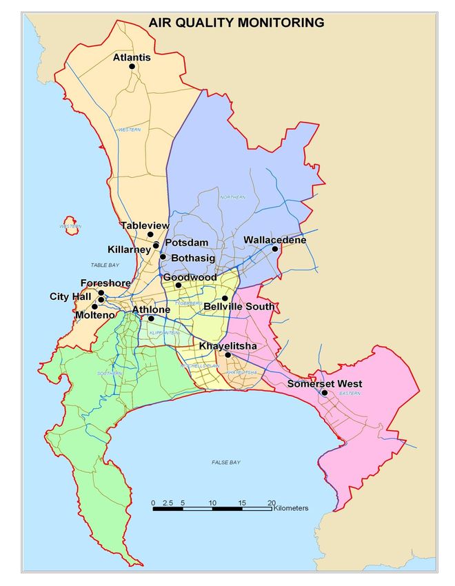
560                                    B. J. Abiodun et al.: The transport of atmospheric NOx and HNO3 over Cape Town

compounds (VOCs) in the presence of heat and sunlight pro-
duces ozone, a major component of smog. It is well known
that smog and ozone cause nose and throat irritation, and
eventually death. Ozone can also damage vegetation and re-
duce crop yields. Cape Town, Africa’s most popular tourist
city with about 3.5 million people (StatsSA, 2012), is usu-
ally covered with smog (called brown haze) in winter. Sev-
eral studies (e.g. Wicking-Baird et al., 1997) have linked the
brown haze to unpleasant odours, health effects and visibility
impairment in the city.
   A combination of geographical and meteorological factors
makes Cape Town favourable for the accumulation of air pol-
lutants. The location of Cape Town (33.9◦ S, 18.4◦ E) at the
southwestern tip of Africa (Fig. 1) influences the wind pat-
terns which it experiences. The city is bordered by the Table
Mountain complex to the southwest, False Bay to the     south,
                                                      Figure  1: Map of southern Africa showing Cape Town area (blue box) at the south western tip o
                                                                     Fig. 1. Map of southern Africa showing the Cape Town area (blue
and Table Bay to the west. At this subtropical latitude,  calm
                                                      South  Africa and the Mpumalanga Highveld (red box), the most industrialised area in Sout
                                                                     box) at the southwestern tip of South Africa and the Mpumalanga
conditions are sometimes produced over the city under Africa, at north eastern part of South Africa.
                                                          stag-      Highveld (red box), the most industrialised area in South Africa, in
nant anticyclonic flows. The subsidence temperature inver-           the northeastern part of South Africa.
sion suppresses vertical exchange of air and pollutants dur-
ing most periods of the year. In addition, radiative cooling
at night produces a stable layer at the surface to form sur-
face inversion, which prevents the vertical dispersion of pol-
lutants during the early mornings. The South Atlantic anti-          ported from remote sources to Cape Town. Since secondary
cyclone and the cold Benguela Current induce surface inver-          pollutants like HNO3 can be transported by wind to cause
sion, which strengthens over the Cape Town (Preston-Whyte            health impacts far from their original sources, it is impor-
et al., 1977). Owing to the temperature contrast between the         tant to investigate how pollutants transported from remote
cold Bengula Current and the warm land, sea breezes develop          sources in South Africa can contribute to the air-quality prob-
during the day and this traps pollutants within the Cape Town        lem in Cape Town. This paper addresses how NOx and HNO3
basin. Berg winds, which occur when a high-pressure system           transported from the Mpumalanga Highveld (the most indus-
over Kwazulu-Natal is associated with a high-pressure sys-           trialised region in South Africa) can accumulate over Cape
tem over the Western Cape with an approaching cold front,            Town.
favour brown haze episodes, because the warm northeast-                 The Mpumalanga Highveld accounts for 90 % of South
erly reduces dew-point temperature during the night (Jury            Africa’s emission of nitrogen oxides and other gases (Col-
et al., 1990). Consequently, extreme high-pollution events           lett et al., 2010). Previous studies (Freiman and Piketh, 2003;
occur from April to September; and, whenever the brown               Piketh et al., 2002) have considered regional scale transport
haze occurs during this period, it extends over most of Cape         and recirculation of pollutants emitted from the Highveld
Town and shifts according to the prevailing wind direction           (using trajectory models with reanalysis data with low reso-                  2
(Wicking-Baird et al., 1997).                                        lution) and showed that most of the pollutants from the High-
   Many studies have investigated pollution over Cape Town,          veld are transported to the Indian Ocean by the westerlies, at
but their focus has been on the influence of locally emitted         700 hPa.
pollutants. Wicking-Baird et al. (1997) showed that vehicles            However, since the Mpumalanga Highveld is located
are the principal source of pollution in Cape Town, account-         northeast of Cape Town, a persistent low-level, northeasterly
ing for about 65% of the brown haze. Local emitting indus-           flow over South Africa can transport the pollutants from the
tries also contribute considerably, accounting for about 22%         Highveld to Cape Town. Such a transport has not been cap-
of the brown haze. The use of wood for fires by a large sec-         tured by previous studies, which used low resolution atmo-
tor of the population accounts for about 11% of the brown            spheric data in trajectory models. In addition, trajectory mod-
haze, and natural sources, such as wind-blown dust and sea           els cannot account for chemical reactions that occur during
salt, contribute about 2 % towards the brown haze. Walton            the transport of air pollutants, making it difficult to account
(2005) identified the Caltex Oil Refinery and Consol Glass           for the concentration of primary and secondary pollutants
as the two main sources of pollution in the city, while the          separately. Meanwhile, in some cases, the concentration of
Cape Town Central Business District, Cape Town Interna-              the secondary pollutants may be higher than that of their pre-
tional Airport, and townships of Khayelitsha and Mitchell’s          cursors. In the present study, a high-resolution atmospheric-
Plain are also major sources. However, none of these previ-          chemistry model that accounts for the influence of topogra-
ous studies accounted for the contribution of pollutants trans-      phy, atmospheric conditions, and chemical reactions among

Atmos. Chem. Phys., 14, 559–575, 2014                                                    www.atmos-chem-phys.net/14/559/2014/
B. J. Abiodun et al.: The transport of atmospheric NOx and HNO3 over Cape Town 561
the atmospheric gasses is used to investigate the transport of pollution for the City Hall station, which is located oppo-
pollutants from the Mpumalanga Highveld to Cape Town. site the city’s busy taxi rank, bus station and rail terminus.
NOx concentration in the atmosphere is essentially the to- Goodwood is a mixed residential and commercial area with
tal concentration of nitric oxide (NO) and nitrogen dioxide nearby industry to the southeast and southwest. The nearby
(NO2 ), while the acid derivate, nitric acid (HNO3 ), is an ox- national road, the N2, carries commuter traffic from Cape
idative product of NOx , as shown in Reactions (R1)–(R4). Town’s northern suburbs to the City, and another busy na-
tional road, the N7, passes along the south side of this area.
NO + O3 → NO2 + O2 (R1)
Road traffic near these two stations is congested during the
NO2 + O → NO + O2 (R2) morning and evening commute. Although located near arte-
NO2 + OH → HNO3 (R3) rial roads, Bothasig and Tableview stations experience less
2NO2 + H2 O → HNO2 + HNO3 (R4) traffic-sourced pollution than the City Hall station, because
the number of commuters on the arterial roads is lower.
The ratio of NO to NO2 is determined by ozone availabil- The data used for this study comprises the hourly aver-
ity and sunshine (or temperature); and nitrous acid and nitric age of NO, NO2 and NOx concentrations, wind speed, wind
acid are produced by reaction of NO2 with moisture/water direction, and temperature for 10 years (2000–2009). The
Eq. (4). Nitrous acid is essentially dominant in heterogenous data were analysed to identify temporal variation of concen-
phase, while in gaseous phase condition, nitric acid domi- trations and associated atmospheric conditions to the peaks.
nates (Seinfeld and Pandis, 2006). Although production of Diurnal variation was analysed to investigate the concentra-
NOx from combustion of nitrogen is characterized by high tion peaks and the contribution of the atmospheric condi-
activation energy, 320kcal/mol (Dean and Bozzelli, 2000), tions. Monthly mean concentrations of pollutants and clima-
the sensitivity of the reaction to temperature is not only due tological variables were used to identify the influence of sea-
to the high activation energy, but also to increasing concen- sonal variation. Monthly temperature and rainfall data from
tration of oxygen atoms during the combustion. Most of the the Climate Research Unit (CRU; Mitchell and Jones, 2005)
reactions in Reactions (R1)–(R4) proceed at fairly low acti- were analysed to supplement the station data in validating the
vation energies, thus promoting abundant NOx and/or acids model simulation.
in the atmosphere. For example, the activation temperature
of Reaction (R1) is 210 K (Sander et al., 2011), indicating
that the reaction is feasible even at sub-zero temperatures. 3 Model descriptions and set-ups
The aim of the present study is to examine the transport
of NOx and HNO3 over South Africa and to investigate how The study applied the International Centre for Theoretical
pollutants from the Mpumalanga Highveld may contribute to Physics (ICTP) Regional Climate model (version 4) with
air pollution in Cape Town. The study combines an analysis chemistry (hereafter, RegCM) to simulate the climate and
of station observations and regional climate model simula- pollution transport over Southern Africa (Fig. 3a). The model
tion to achieve the aim. It calculates the flux budget of the allows online coupling of atmospheric and chemistry param-
pollutants over Cape Town and investigates the atmospheric eters. The climate component has been successfully tested
conditions that favour accumulation of pollutants over the over Southern Africa (Sylla et al., 2009). RegCM is a hydro-
city. The methodology used in the study is discussed in static, sigma-coordinate model (Pal et al., 2007; Giorgi et al.,
Sect. 2, results and discussions are in Sect. 3, while the con- 2012). The model has various options for physics and chem-
clusion is in Sect. 4. istry parameterisations. In the present study, the model used
the CCM3 (Kiehl et al., 1996) radiation scheme for radia-
2 Methodology tion calculations, the (Grell et al., 2005) mass-flux cumulus
scheme with Fritsch and Chappell (1980) closure for convec-
2.1 Observed data tion, and the Holtslag and Boville (1993) scheme for plane-
tary boundary-layer parameterisation.
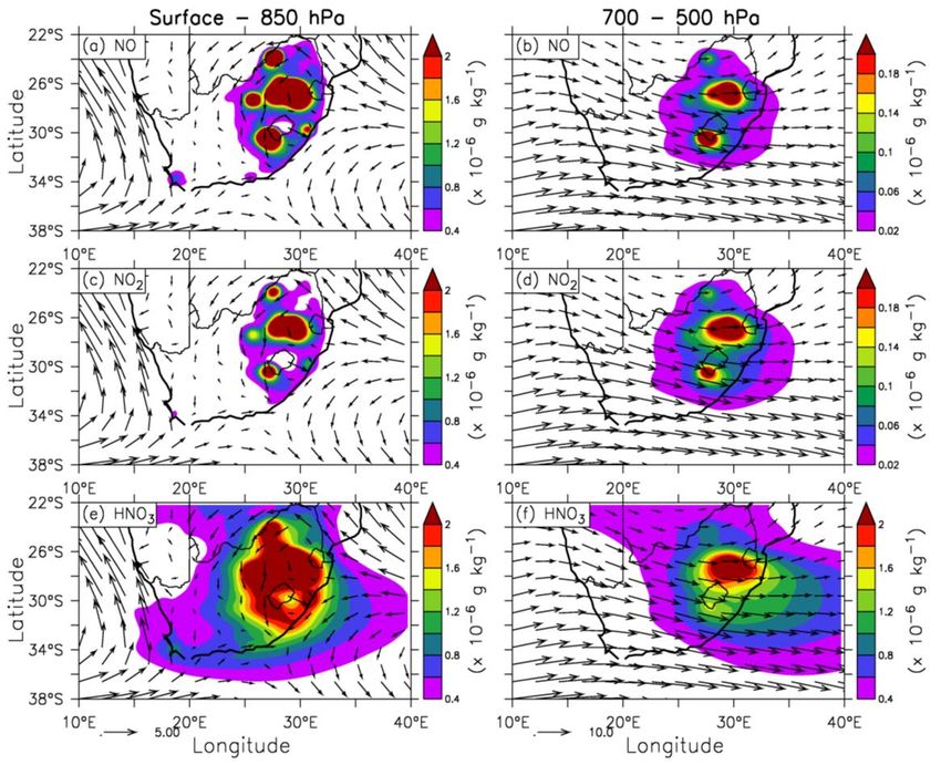
This study used meteorological and pollution data from four Surface-layer, land–atmosphere interactions were rep-
stations within the Cape Town air-quality monitoring net- resented with BATS1E (Biosphere-Atmosphere Transfer
work (Fig. 2). The network comprises 12 stations within a Scheme) (Dickinson et al., 1993), which is based on Monin–
500 km2 area and measures ambient concentrations of se- Obukhov similarity relations (Monin and Obukhov, 1954).
lected pollutants considered hazardous to human health and For the chemistry routines, the photochemical Carbon Bond
ecology (City of Cape Town, 2005), as well as relevant me- Mechanism-Z (CBM-Z) (Zaveri and Peters, 1999) was used.
teorological parameters that might explain high concentra- Photolysis is based on the Tropospheric Ultraviolet-Visible
tions. Model (TUV) scheme developed by Madronich and Flocke
The stations with relevant observations for the period of (1999). For dry deposition the model used the CLM4 (Com-
the study are City Hall, Goodwood, Bothasig and Table- munity Land Model 4) developed after Wesley (1989),
view (Fig. 2). Vehicular emissions are the prime source of and wet deposition follows the MOZART global model
www.atmos-chem-phys.net/14/559/2014/ Atmos. Chem. Phys., 14, 559–575, 2014
562                                                  B. J. Abiodun et al.: The transport of atmospheric NOx and HNO3 over Cape Town

                                                                                                  values over Mpumalanga and over Cape Town for this pe-
                                                                                                  riod are shown in Fig. 3c. The simulation covers a period of
                                                                                                  four years and three months (i.e. October 2000–December
                                                                                                  2004). The first three months’ simulations were discarded as
                                                                                                  model spin-up, while the remaining four years’ simulations
                                                                                                  were analysed for the study.

                                                                                                  3.1     Pollutants flux budget

                                                                                                  Flux budget analysis was used to calculate the net flux of the
                                                                                                  pollutants (NOx and HNO3 ) over Cape Town and to examine
                                                                                                  whether the city is a source or sink for the pollutants. The
                                                                                                  pollutant net flux (FNet ) is defined as:

                                                                                                  FNet = (FE − FW ) + (FN − FS )                              (1)

                                                                                                  where FE , FW , FN , and FS are the pollutant fluxes at the
                                                                                                  eastern, western, northern and southern boundaries of Cape
                                                                                                  Town (Fig. 1), respectively.
                                                                                                     A positive zonal flux (FE or FW ) implies a westerly pol-
                                                                                                  lutant flux (i.e. pollutant flux from the westerly direction),
                                                                                                  while a negative zonal flux means the opposite. A positive
                                                                                                  meridional flux (FN or FS ) denotes a southerly pollutant flux
                                                                                                  (i.e. pollutant flux from the southerly direction), while a neg-
                                                                                                  ative zonal flux means the opposite. A positive net flux indi-
                                                                                                  cates divergence of a pollutant over the city, meaning that the
                                                                                                  city is a net source for the pollutant. A negative net flux in-
                                                                                                  dicates convergence (or accumulation) of pollutants over the
Figure
  Fig.2:2.Map  of the
             Map     ofCape
                        theTown,
                             Capeshowing
                                   Town,theshowing
                                              air quality the
                                                          network
                                                              air inquality
                                                                     Cape Town and the location
                                                                            network    in         city, meaning that the city is a net sink for the pollutant.
of four observation stations (Bothasig, City Hall, Goodwood and Tableview) used in the study
  Cape    Town     and   the location   of  four   observation     stations (Bothasig,
(source: http://web1.capetown.gov.za/web1/cityairpol). The colour code indicates different
suburbs
  City inHall,
           the city.
                  Goodwood and Tableview) used in the study (source:
                                                                                                  4     Results and discussion
  http://web1.capetown.gov.za/web1/cityairpol). The colour code in-                         24
  dicates different suburbs in the city.
                                                                                                  This section presents and discusses the results of the study
                                                                                                  in three parts. The first part describes the temporal (diurnal
                                                                                                  and seasonal) variation of the observed pollutant concentra-
  (Emmons et al., 2010). Shalaby et al. (2012) presents a de-
                                                                                                  tions and meteorological variables at the four stations (City
  tailed description of the gas-phase chemistry in RegCM.
                                                                                                  Hall, Goodwood, Bothasig and Tableview) within the city
     The RegCM simulation was set up with a 35km horizontal
                                                                                                  (see Fig. 2). The second part compares RegCM simulation
  resolution. The simulation domain centres on 33◦ S and 24◦
                                                                                                  (pollutant concentrations and meteorological variables) with
  E and extends, with the Lambert conformal projection, from
                                                                                                  the observed data. The third part discusses the characteristics
  16.62◦ W to 54.41◦ E and from 10.5◦ S to 40.45◦ S (Fig. 3a).
                                                                                                  of the simulated NOx (NO and NO2 ) and HNO3 over Cape
  In the vertical, the domain spans 18 sigma levels, with high-
                                                                                                  Town.
  est resolution near the surface and lowest resolution near the
  model top. Initial and lateral boundary meteorological condi-                                   4.1     Observed nitrogen oxides and atmospheric
  tions were provided by ERA-Interim 1.5◦ × 1.5◦ gridded re-                                              conditions over Cape Town
  analysis data from ECMWF (European Centre for Medium-
  Range Weather Forecasts). The global emissions data sets                                        4.1.1    Diurnal variation
  (1◦ × 1◦ resolution) used in the simulation were derived
  from the Coupled Model Intercomparison Project Phase                                            The diurnal cycle of NO, NO2 , NOx (Fig. 4) shows that the
  5 (CMIP5) RCP (Representative Concentration Pathways,                                           pollutants have the highest concentration at City Hall and
  Moss et al., 2010; van Vuuren et al., 2011) emission, pro-                                      the lowest concentration at Tableview. This is because City
  vided with the standard RegCM package (http://clima-dods.                                       Hall is located in the heart of the city where the emission
  ictp.it/data/d8/cordex/RCP_EMGLOB_PROCESSED). The                                               of NO from daily anthropogenic activity (traffic, industrial,
  emissions data set has monthly variation; the horizontal dis-                                   business) is greatest. The diurnal variation of NO concentra-
  tribution of NO emission over Southern Africa, averaged be-                                     tion (Fig. 4a) shows two peaks (morning and evening peaks)
  tween 2001 and 2004, is shown in Fig. 3b, while the monthly                                     at City Hall, but one peak (in morning) at other stations

  Atmos. Chem. Phys., 14, 559–575, 2014                                                                              www.atmos-chem-phys.net/14/559/2014/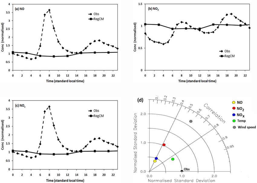
B. J. Abiodun et al.: The transport of atmospheric NOx and HNO3 over Cape Town                                                     563

                Figure 3: (a) RegCM simulation domain indicating the topography (in meters) of southern Africa
Fig. 3. (a) RegCM simulation domain indicating the topography (in metres) of southern Africa as seen by the model; (b) the annual mean
of NO emission as   seen
                 over     by the
                       South     model;
                             Africa used (b) themodel;
                                         in the  annual(c)
                                                        mean   of NO emission
                                                           the temporal variation over South
                                                                                   of NO     Africa
                                                                                         emission   used
                                                                                                  over    in the model;
                                                                                                       Mpumalanga   and Cape Town in
2001–2004.      (c)  the temporal variation  of NO  emission  over Mpumalanga      and Cape  Town  in 2001  - 2004.

                                                                                                                      25
Fig. 4. Diurnal variation
           Figure         of observed
                    4: Diurnal         (a) NO,of(b)
                                  variation         NO2 , (c) (a)
                                                 observed     NOxNO,
                                                                  (d) temperature,
                                                                      (b) NO2, (c)andNO
                                                                                      (e) wind speed at four monitoring stations in Cape
                                                                                        x (d) temperature, and (e) wind
Town. The values are for all seasons (2001–2008).
           speed at four monitoring stations in Cape Town. The values are for all seasons (2001-2008).

(Bothasig, Goodwood, and Tableview). The morning peaks                60 µg m−3 ) occurs at 16:00 SLT. Although Bothasig, Good-
(City Hall: 280 µg m−3 ; Goodwood: 120 µg m−3 ; Bothasig:             wood, and Tableview show no evening peak, the NO concen-
60 µg m−3 ; and Tableview: 20 µg m−3 ) occur at 08:00 SLT             tration is higher in the evening (18:00–20:00 SLT) than in the
(Standard Local Time), while the evening peak (City Hall:             afternoon.

www.atmos-chem-phys.net/14/559/2014/                                                       Atmos. Chem. Phys., 14, 559–575, 2014
564                                     B. J. Abiodun et al.: The transport of atmospheric NOx and HNO3 over Cape Town

Fig. 5. The monthly
         Figure     mean monthly
                 5: The  of observedmean
                                    (a) NO,of(b) NO2 , (c) NO
                                               observed     (a)x ,NO,
                                                                  (d) Temperature, (e) wind
                                                                        (b) NO2, (c)   NOx,speed, and (d) wind direction
                                                                                             (d) Temperature,            at four monitoring
                                                                                                                   (e) wind
stations in Cape Town (2001–2008).
        speed, and (d) wind direction at four monitoring stations in Cape Town (2001 -2008).

   The morning peaks and the evening peak at City Hall can                 However, the diurnal variation of meteorological variables
be attributed to the high commuter traffic in the city, be-             may also play an important role in the diurnal variation of
cause people rush to work and school in the morning (around             the pollutants’ concentration. The diurnal variation in wind
08:00 SLT) and return home in the evening (16:00 SLT).                  speed (Fig. 4e) and surface temperature (Fig. 4d) may en-
However, the concentration peak is higher in the morning                hance the concentrations of the pollutants in the morning and
than in the evening, because the traffic rush is greater in the         lower them in the afternoon. For instance, the weak surface
morning than in the evening, as schools and offices open at             wind speed in the morning (Fig. 4b) may lead to the accumu-
same time in the morning (08:00 SLT) but close at different             lation and higher concentration of NO, while the higher wind
times in the afternoon.                                                 speed in the afternoon may reduce NO concentration.
   The diurnal variation of NO2 differs from that of NO.                   Besides, in the morning, the surface inversion layer (in-
At City Hall, the diurnal variation of NO2 shows no dis-                duced by low surface temperature from the nocturnal radia-
tinct peak; instead, it shows a uniform concentration (about            tive cooling) can inhibit vertical mixing of the NO. In the
50 µg m−3 ) during the day (08:00–18:00 SLT) and a lower                afternoon, the surface heating increases the surface temper-
concentration (about 20 µg m−3 ) at night. In contrast, the             ature and the development of a mixing layer will erode the
diurnal variation of NO shows two distinct peaks at other               inversion layer. Hence, pollutants trapped below the surface
stations (Goodwood: 25 µg m−3 ; Tableview and Bothasig:                 layer will rise and disperse, reducing the NO concentration
18 µg m−3 ) in the morning (08:00 SLT) and in the evening               in the afternoon.
(19:00 SLT). However, at all stations, the NO2 concentration               In contrast, the increase in NO2 concentration in afternoon
is smaller than that of NO, because NOx are mainly emitted              may be attributed to an increase in temperature which can
in the form of NO, which is later oxidized to NO2 by different          enhance the generation of more NO2 owing to chemical re-
photochemical reactions (Eq. 1). The rate of these reactions            action (see Eq. 1). This could further explain why the NO2
depends on favourable atmospheric conditions. Nevertheless,             concentration is much higher at the City Hall (where27 maxi-
since the magnitude of NO concentration is about five times             mum temperature is about 27◦ C) than at Bothasig (where the
higher than that of NO2 (Fig. 4), the diurnal variation of NOx          maximum temperature is about 22◦ C).
(NO + NO2 ) follows that of NO.

Atmos. Chem. Phys., 14, 559–575, 2014                                                       www.atmos-chem-phys.net/14/559/2014/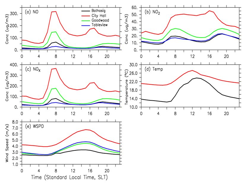
B. J. Abiodun et al.: The transport of atmospheric NOx and HNO3 over Cape Town                                                      565

Fig. 6. Comparison of the simulated (RegCM) and observed diurnal variation of (a) NO, (b) NO2 , and (c) NOx concentrations. (d) shows the
Taylor diagram, which uses correlation coefficient and normalised standard deviation to compare variations in the simulated and observed
(Obs) daily mean NO, NO2 , NOx , temperature (Temp), and wind speed. The average observation over the four stations is indicated as Obs.
The normalised standard deviations are obtained by dividing the simulated and observed standard deviations with the observed standard
deviation.

4.1.2   Seasonal variation                                             centration and atmospheric conditions that favour NO2 pro-
                                                                       duction. For instance, less NO concentration limits the pro-
                                                                       duction of NO2 in January (when the temperature is most
The concentration of the pollutants also varies with seasons           favourable for the production), and less favourable atmo-
(Fig. 5). The seasonal variations of the atmospheric con-              spheric conditions prevent a peak concentration of NO2 in
ditions may play a major role in the seasonal variation of             June, when the NO concentration reaches its peak.
the pollutants’ concentration. At all stations, NO shows a
maximum concentration (City Hall, 200 µg m−3 ; Goodwood,               4.2   Model validation
100 µg m−3 ; Bothasig, 100 µg m−3 ; Tableview, 30 µg m−3 ) in
early winter (June) and a minimum concentration (City Hall:            The diurnal variation of the simulated pollutants (NO, NO2
80 µg m−3 ; Goodwood, Bothasig and Tableview: 20 µg m−3 )              and NOx ) shows a weaker diurnal variation than the observed
in summer (December–February). Nevertheless, the seasonal              (Fig. 6). This is because the monthly emissions data used
variation is most pronounced at City Hall and least defined at         in simulation did not account for diurnal variation of the lo-
Tableview (Fig. 5a). The occurrence of maximum concentra-              cal sources (i.e. the high commuter traffic in the city) dis-
tion of NO in winter can be attributed to the weak wind speed          cussed earlier (see Sect. 3.1.1). The simulated diurnal varia-
and low surface temperature during this period, as both con-           tion shows the lowest concentration during the day (between
ditions do not favour the pollutant dispersion and its conver-         09:00 and 14:00 SLT), when the enhancement of boundary-
sion to NO2 through the reaction in Eq. (1).                           layer vertical mixing reduces the pollutants’ concentration at
   The seasonal variation of NO2 (and NOx ) is similar to that         lower level. This is consistent with a decrease in the observed
of NO (Fig. 5), except that: (1) the concentration of NO2 is           NO and NOx concentration between 12:00 and 15:00 SLT.
smaller than that of NO; (2) at City Hall, the maximum con-               The daily mean concentration of the simulated NO shows
centration of NO2 extends over more months (March–July)                a weak correlation with the observed values, and the standard
than that of NO; and (3) at Tableview, the maximum concen-             deviation is lower than the observed (Fig. 6). The correlation
tration of NO2 is in March–May instead of in June (as for              coefficient is about 0.4, and the normalised standard devi-
NO). The occurrence of maximum concentration of NO2 in                 ation (i.e. simulated standard deviation divided by the ob-
March–July can be attributed to a balance between NO con-              served standard deviation) is 0.4. The simulated correlation

www.atmos-chem-phys.net/14/559/2014/                                                       Atmos. Chem. Phys., 14, 559–575, 2014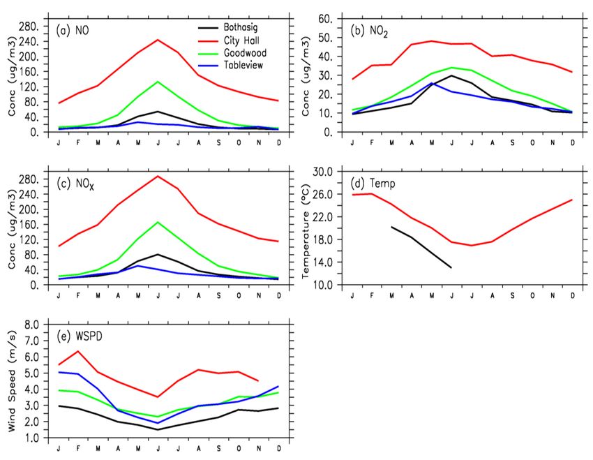
566                                      B. J. Abiodun et al.: The transport of atmospheric NOx and HNO3 over Cape Town

Fig. 7. Seasonal Figure    7: Seasonal
                   variation            variation
                              of observed         of observed
                                           and simulated      and(b)simulated
                                                         (a) NO,       NO2 , (c)(a)
                                                                                 NONO,    (b)Temperature
                                                                                    x , (d)   NO2, (c) NO(◦ xC),
                                                                                                             , (d)(e) Wind Speed (m s−1 ), and
                       −1
(f) Rainfall (mm day ). The NO,      NO2 and NOx concentration   are normalised with their annual  mean values. The average observation over
                  Temperature (oC),    (e) Wind Speed (m s-1), and    (f) Rainfall (mm day-1). The    NO, NO2 and NOx
the four stations is indicated as Obs (station).
                 concentration are normalised with their annual mean values. The average observation over the
                 four stations is indicated as Obs (station).
between the observed and simulated NO2 is also 0.4, but the              discrepancy may be attributed to the winter rainfall, which
normalized standard deviation (about 1.0) is much better than            cleanses the atmosphere of any accumulated pollutants.
that of NO. The normalized standard deviation of NOx (0.50;              Since RegCM underestimates the local emission of the pollu-
Fig. 6d) falls between those of NO and NO2 , but the cor-                tants, the building up of the pollutants in the atmosphere, af-
relation coefficient is also 0.4. There is a better correlation          ter the cleansing by the winter rain, may take a longer time in
between the simulated and observed atmospheric variables                 the model than in the observation. The simulated rainfall and
than with the pollutants’ concentrations, suggesting that the            temperature show a good agreement with CRU observation,
weak correlation between the observed and simulated pol-                 except that the model underestimates temperature in sum-
lutant concentration may be due to the RegCM chemistry.                  mer months, overestimates rainfall in winter, and underesti-
However, the RegCM shows its best performance in simu-                   mates rainfall in winter. However, the model underestimates
lating temperature – the correlation coefficient is 0.85 and             the concentrations of pollutants in winter (May–August) and
the normalized standard deviation is 0.8. The discrepancy be-            overestimates them in other months. The simulated rainfall
tween simulated pollutant and observation may be due to the              and temperature show a good agreement with CRU obser-
low resolution of the simulation and low resolution of the               vation, except that the model underestimates29temperature in
emission data sets with no diurnal variation. These would in-            summer months, overestimates rainfall in summer, and un-
fluence the capability of the model ability in simulating the            derestimates rainfall in winter.
spatial and temporal (i.e. diurnal and daily) variations of pol-
lutants in the city.                                                     4.3     Characteristics of the simulated pollutant and
   The seasonal variation of the simulated pollutants’ con-                      atmospheric conditions over South Africa
centration is similar to the observed, except that simulated
peak concentration lags the observed peak by two months                  4.3.1    Annual mean
(Fig. 7). The simulated peak concentrations are in April,
while the observed peak concentrations are in June. This                 RegCM simulates the hot spots of NO, NO2 and HNO3 con-
                                                                         centrations over the northeast of South Africa (Fig. 8). The

Atmos. Chem. Phys., 14, 559–575, 2014                                                        www.atmos-chem-phys.net/14/559/2014/
B. J. Abiodun et al.: The transport of atmospheric NOx and HNO3 over Cape Town 567
-6 -1
Figure
Fig. 8. RegCM4 8: RegCM4
simulated annual simulated annual concentration
mean (2001–2004) mean (2001for -2004)
NO (×concentration forpanels),
10−6 g kg−1 ; top NO (x NO10 2 g(×kg ; top
10−6 g kg−1 ; middle
panels) and HNO3 (× 10−6 g kg−1-6; bottom -1 panels) at low level (surface–850 hPa; left
-6 panels)
-1 and middle level (700–500 hPa; right panels)
panels), NO2 (x 10 g kg ; middle panels) and HNO3 (x 10 g kg ; bottom panels) at low-level
over South Africa. The corresponding wind speeds are shown with arrows; the arrows at the bottom of the bottom panels (e and f) show the
5 m s−1 and
wind scale of(surface – 850
10 m s−1 ,left
hPa; respectively.
panels) and middle-level (700 -500 hPa; right panels) over South Africa.
The corresponding wind speeds are shown with arrows; the arrows at bottom of the bottom
maximum concentration
panels (e andoff) NO
show(about
the wind 10−6 gofkg5−1
30 × scale m) sis-1 andtants
10 mfrom the hot spots towards the Indian Ocean, while the
s-1, respectively.
over the Mpumalanga Highveld, the area of intense indus- anticyclonic flow recycles the pollutant over southern Africa.
trial activities in South Africa (Collett et al., 2010). The At lower level, the wind pattern is dominated by northerly
maximum concentration of NO2 (about 5.0 × 10⁻⁶ g kg−1 ) and northeasterly flows over the continent, southwesterly and
is also over the Mpumalanga Highveld, but the magnitude southeasterly flows over the Atlantic Ocean, and easterly
is lower than that of NO, because NO2 is formed by oxi- flows over the Indian Ocean. The northerly and northeast-
dation of NO (see Eq. 1). The maximum concentration of erly flows transport pollutants from the hot spots toward the
HNO3 (about 5.0 × 10⁻⁶ g kg−1 ) is also lower than that of southern coast and to Cape Town. The northerly flows con-
NO, but HNO3 concentrations cover a wider area than those verge with the southerly winds along the southern coast. The
of NO and NO2 concentrations. For instance, the contour of convergence produces weak winds and induces accumulation
0.5 × 10⁻⁶ g kg−1 in HNO3 covers almost the entire country, of the pollutants over the southwestern half of South Africa,
but that of NO and NO2 are limited to the eastern part of the along the southern coasts, and over Cape Town. The east-
country (Fig. 8). This is because most of the NO and NO2 are erly flow transports fresh air from the Indian Ocean to the
converted to HNO3 as they are transported away from the hot eastern coast, but also picks up pollutants from the hot spots
spots. and transports them along the coastline towards Cape Town
The model simulation shows a difference in the trans- area. Hence, while the upper-level winds (westerlies) trans-
port of the pollutants (NO, NO2 and HNO3 ) at lower level port fresh air eastward from the Atlantic Ocean over the Cape
(surface–850 mb) and at upper level (700–500 mb) (Fig. 8). Town area, the surface winds (easterlies and northeasterlies)
30
At the upper level (i.e. 700 hPA), the wind pattern is domi- transport pollutants from the Mpumalanga Highveld toward
nated by a westerly flow with a weak trough over the western the city.
coast and an anticyclonic flow over the northeast of South The emphases of previous studies have been on the east-
Africa. At this level, the westerly flow transports most pollu- ward transport of Highveld pollutants by the upper-level
westerly flow and on the recirculation of the pollutants over
www.atmos-chem-phys.net/14/559/2014/ Atmos. Chem. Phys., 14, 559–575, 2014568 B. J. Abiodun et al.: The transport of atmospheric NOx and HNO3 over Cape Town
-6 -1
Figure
Fig. 9. Monthly 9: Monthly
anomalies anomalies
of the simulated of3the
HNO concentration 10−63gconcentration
simulated(×HNO kg−1 ) over South
(xAfrica.
10 g kg ) over South
Africa.
southern Africa by the anticyclones. For instance, Freiman 4.3.2 Seasonal variation
and Piketh (2003) show that 39 % of pollutants from the
Highveld are transported to the Indian Ocean, 33 % are re- The simulated HNO3 over South Africa exhibits a seasonal
cycled over the sub-continent, and only 6 % are transported variability in which atmospheric condition plays a major role
by the northerly flow to the south of the Indian ocean. The (Fig. 9). The highest variability in HNO3 occurs over the
present results suggest however that the amount of HNO3 Mpumalanga Highveld, with positive anomalies in April–
transported from the Highveld pollutants southward (and to- September and negative anomalies in October–March. The
wards Cape Town) may be substantial, and given that the anomalies can be attributed to the prevailing atmospheric
winds are weaker at lower level than at upper level, and the conditions during the periods. In summer (October–January),
pollutant concentrations are higher at low level than at upper the inversion layer over the eastern coast is elevated above the
level, it is important to have a better understanding of pollu- mountain range (i.e. the escarpment). This allows the easterly
tants’ transport at low level, especially over South Africa. flow from the Indian Ocean to penetrate inland and dilute
Using a high-resolution (about 1.5 × 1.5 km) simulation the concentration of HNO3 over the Mpumalanga Highveld
over the Western Cape, Jury et al. (1990) attributes the weak (Fig. 10). The reverse is the case in winter (April–August),
wind over the Western Cape to convergence of land and sea when the inversion layer is lower than the peak of the es-
breezes; the present study suggests however that the weak carpment. The easterly flow cannot penetrate inland with the
wind may be due to convergence of synoptic scale flows, be- fresh air; instead, it deflects around the mountain ranges,
cause the lower resolution (30 × 30 km) simulation used in southward along the coastline or northward toward 31 Mozam-
the present study cannot resolve land and sea breezes, yet bique. Rainfall may also lower HNO3 concentrations in sum-
the simulation features the weak wind and further shows that mer, because the eastern part of South Africa experiences
weak wind covers a wider domain than shown in Jury et intense rainfall in summer and the rainfall will cleanse the
al. (1990). atmosphere of HNO3 .
The seasonal variation of HNO3 is weaker over Cape
Town than over the Mpumalanga Highveld, but the anoma-
lies over Cape Town are substantial and are influenced by
transport of HNO3 from the Mpumalanga Highveld region.
Atmos. Chem. Phys., 14, 559–575, 2014 www.atmos-chem-phys.net/14/559/2014/B. J. Abiodun et al.: The transport of atmospheric NOx and HNO3 over Cape Town 569
Fig. 10. Vertical cross section of HNO3 concentration (× 10−6 g kg−1 ; shaded in upper
-6 panels)
-1 and temperature (◦ C; contours in upper
Figure 10: Vertical cross section of HNO 3 concentration (x 10 g kg ; shaded in upper
panels), vertical wind component o(× 100 mb s ; shaded in lower panels), and zonal wind component (m s−1 ; contours
−1 panels)
in lower panels) at
-1
◦ and temperature ( C; contours in upper panels), vertical wind component (x 100 mb s ;
latitude 26 S in January and July. Topography is shown in grey colour and the location of the Highveld indicated withshaded
arrow (↑).
in lower panels), and zonal wind component (m s-1; contours in lower panels) at latitude 26oS in
January and July. Topography is shown in grey colour and the location of the Highveld indicated
The seasonal variability shows strong positive anomalies of April–August but inward fluxes in other months. However, in
with arrow (↑).
HNO3 in February–April and weaker negative anomalies in most cases, the magnitudes of the outward fluxes at the west-
other months. The months with the positive anomalies fea- ern boundary are greater than the magnitude of outward or
ture easterly and northeasterly flows transporting HNO3 from inward fluxes at other boundaries. Hence, climatologically,
the Mpumalanga Highveld toward Cape Town, while the Cape Town is a net exporter of the pollutants, and most of
months with negative anomalies are characterized by south- the pollutants from the city are exported through the western
westerly winds transporting fresh maritime air towards Cape boundary. However, as it will be shown later, the situation is
Town. Note that, unlike the eastern part of South Africa, different during extreme pollution events.
Cape Town experiences its intense rainfall in winter. The re-
moval of HNO3 from the atmosphere by the winter rainfall 4.3.3 Transport of pollutants during extreme events in
may contribute to the negative anomalies in winter months. Cape Town
Table 1 presents the monthly budget of pollutants’ (NO,
NO2 , NOx and HNO3 ) fluxes over Cape Town at lower level. The time series of the simulated pollutants’ concentration
The monthly mean of the net flux is positive for all the pollu- over Cape Town (Fig. 11) shows that the extreme concentra-
tants in each month. That means that, over the city, the mag- tion events (defined as 99 percentiles; ≥ 3.3 × 10⁻⁶ g kg−1
nitude of outgoing pollutants is greater than the magnitude of for NOx ; ≥ 2.8 × 10⁻⁶ g kg−1 for HNO3 ) mostly occur in
incoming pollutants; so, Cape Town is a source for the pollu- April. For NOx (Fig. 11c), the extreme events occur once
tants. For all the pollutants, the maximum net flux occurs in in 2001 but twice in 2003 and 2004. For HNO32 3 , the extreme
April and the minimum in November, January, or August. events occur once 2001, thrice in 2002 and twice in 2003 and
The western boundary of the city always experiences out- 2004. However, the extreme events for NO x and HNO 3 rarely
ward fluxes of the pollutants, except in June when it expe- occur on the same day, suggesting that, in Cape Town, the at-
riences inward fluxes of HNO3 (Table 1). Its maximum out- mospheric conditions that induce NO x extreme events may
ward flux occurs in January. The northern boundary features be different from those that induce HNO 3 extreme events.
inward fluxes for the pollutants in April–August but outward The time difference may also be attributed to the chemical
fluxes in the remaining months. The reverse is the case at reactions which form HNO3 from NOx .
the southern boundary, where there are outward fluxes in
www.atmos-chem-phys.net/14/559/2014/ Atmos. Chem. Phys., 14, 559–575, 2014570 B. J. Abiodun et al.: The transport of atmospheric NOx and HNO3 over Cape Town
Table 1. The low-level flux budget of pollutants (NO, NO2 , NOx and HNO3 ) over Cape Town for each month, showing the inward and
outward fluxes at the western (FW ), eastern (FE ), southern (FS ) and northern (FN ) boundaries of Cape Town and the net flux (FNet ) over
the city. A positive zonal flux (FE or FW ) implies a westerly flux (i.e. a flux from a westerly direction), while a negative zonal flux means
the opposite. A positive meridional flux (FN or FS ) denotes a southerly flux (i.e. a flux from a southerly direction), while a negative zonal
flux means the opposite. Inward fluxes (from any boundary or direction) into the city are in bold font, while outward fluxes from the city are
in thin font. A positive FNet indicates divergence (i.e. depletion) of the pollutants over the city, while a negative net flux means convergence
(i.e. accumulation) of the pollutants over the city.
Jan Feb Mar Apr May Jun Jul Aug Sept Oct Nov Dec.
NO
FW −1.9 −2.4 −2.2 −1.3 −0.6 0.0 −0.4 −0.3 −1.1 −1.1 −1.6 −1.7
FE −0.4 −1.0 −0.8 0.3 0.5 0.9 0.6 0.9 0.2 0.2 −0.2 −0.4
FS 1.6 1.5 1.5 −0.4 −0.7 −1.5 −1.2 −0.6 0.3 0.4 1.5 1.4
FN 1.2 1.0 1.6 −0.2 −0.3 −0.7 −0.6 −0.3 0.1 0.4 1.0 1.2
FNet 1.1 0.9 1.5 1.7 1.5 1.7 1.6 1.5 1.2 1.3 0.9 1.0
NO2
FW −1.5 −2.0 −1.8 −1.0 −0.5 0.0 −0.4 −0.3 −0.9 −0.9 −1.3 −1.4
FE −0.3 −0.6 −0.4 0.2 0.3 0.5 0.3 0.4 0.0 0.1 −0.2 −0.2
FS 1.2 1.2 1.2 −0.3 −0.5 −1.0 −0.7 −0.4 0.2 0.3 1.1 1.0
FN 0.8 0.8 1.0 −0.1 −0.2 −0.4 −0.4 −0.2 0.1 0.3 0.7 0.8
FNet 0.9 1.0 1.2 1.4 1.1 1.0 1.0 0.9 0.8 1.0 0.8 0.8
NOx
FW −3.4 −4.4 −4.0 −2.2 −1.1 −0.1 −0.8 −0.6 −2.0 −2.0 −2.9 −3.0
FE −0.7 −1.5 −1.2 0.5 0.8 1.3 1.0 1.3 0.2 0.2 −0.4 −0.6
FS 2.8 2.7 2.7 −0.7 −1.2 −2.5 −1.9 −1.0 0.5 0.6 2.5 2.5
FN 1.9 1.8 2.6 −0.3 −0.6 −1.1 −1.0 −0.5 0.2 0.6 1.7 1.9
FNet 1.9 1.9 2.7 3.1 2.6 2.8 2.6 2.3 2.0 2.2 1.7 1.9
HNO3
FW −3.1 −4.7 −3.7 −1.5 −0.8 0.2 −0.6 −0.5 −2.2 −1.6 −2.6 −2.8
FE −1.7 −3.0 −1.6 0.0 0.0 0.6 0.0 0.2 −1.2 −0.7 −1.1 −1.5
FS 2.8 3.4 3.0 −0.4 −0.7 −1.7 −1.6 −0.7 0.7 0.7 2.5 2.6
FN 1.8 2.1 2.2 −0.3 −0.6 −1.2 −1.7 −0.6 0.0 0.4 1.6 1.7
FNet 0.4 0.4 1.2 1.6 1.0 0.9 0.6 0.8 0.4 0.6 0.5 0.4
The composite of wind flow during extreme pollution southerly flows over Cape Town will provide a favourable at-
events in Cape Town shows a transport of pollutants from mospheric condition for accumulation of the pollutants over
the Mpumalanga Highveld to Cape Town at surface (Fig. 12). the city during the extreme events.
For NOx extreme events, the low-level wind pattern is char- At 700 hPa (Fig. 13), there is a strong anticyclonic flow
acterized by northerly and northeasterly flows, transporting over southern Africa. This anticyclone will produce a strong
the pollutant from the Mpumalanga Highveld towards Cape subsidence over South Africa, and the subsidence will pre-
Town and the south coast. vent a vertical mixing of the pollutants, capping the high
Along the southern coastline, there is a confluence of the concentrations of pollutants close to the surface as they are
northerly flow and easterly flow; and the easterly flow also transported toward from the Mpumalanga Highveld toward
transports pollutants from the eastern part of South Africa to- Cape Town. The synoptic wind patterns that induce the ex-
wards Cape Town. The wind pattern also features a col over treme HNO3 events differ from those that induce the extreme
Cape Town. A col is a relatively neutral area of low pres- NOx events (Fig. 12d). With HNO3 extreme events, the low-
sure between two anticyclones, or a point of intersection of a level wind pattern features a strong northwesterly flow trans-
trough (in cyclonic flow) and a ridge (in anticyclonic flow). porting HNO3 from the Mpumalanga Highveld towards the
It is usually associated with a calm or light variable wind south coast. In addition, it shows a strong easterly flow trans-
which causes stagnation of air flow. A col can cause an ac- porting fresh air from Indian Ocean, but turns poleward as it
cumulation of atmospheric pollution (Stein et al., 2003). The approaches the escarpment, thereby deflecting the fresh air
formation of a col with the convergence of northeasterly and from the continent, at the same time forming a confluence
Atmos. Chem. Phys., 14, 559–575, 2014 www.atmos-chem-phys.net/14/559/2014/B. J. Abiodun et al.: The transport of atmospheric NOx and HNO3 over Cape Town 571
Fig. 11. The time series
Figure 11:ofThe
the simulated pollutants
time series concentration
of the simulated over Cape
pollutants Town in 2001–2004.
concentration The Town
over Cape extremeinvalues – percentiles) are
2001(99
indicated with 2004.
red dashed.
The extreme values (99 percentiles) are indicated with red dashed.
Table 2. The low-level flux budget of pollutants (NO, NO2 , NOx and HNO3 ) during extreme events over Cape Town, showing the inward
and outward fluxes at the western (FW ), eastern (FE ), southern (FS ) and northern (FN ) boundaries of Cape Town and the net flux (FNet ) over
the city. A positive zonal flux (FE or FW ) implies a westerly flux (i.e. a flux from a westerly direction), while a negative zonal flux means
the opposite. A positive meridional flux (FN or FS ) denotes a southerly flux (i.e. a flux from a southerly direction), while a negative zonal
flux means the opposite. Inward fluxes (from any boundary or direction) into the city are in bold font, while outward fluxes from the city are
in thin font. A positive FNet indicates divergence (i.e. depletion) of the pollutants over the city, while a negative net flux means convergence
(i.e. accumulation) of the pollutants over the city.
NO NO2 NOx HNO3
March April March April April March April May
FW −3.1 −0.4 −0.9 −1.0 −0.7 1.4 −0.5 1.0
FE −3.0 −0.7 −0.5 −0.9 −1.4 1.3 0.7 1.1
FS 0.8 −0.9 0.5 0.1 −0.8 −0.8 1.8 −0.6
FN −1.1 −2.0 −0.6 −1.1 −1.6 −0.4 0.8 −1.0
FNet −1.8 −1.3 −0.7 −1.1 −1.4 0.3 0.2 −0.3
flow with the northwesterly flow along the coast. The wind Table 2 shows that Cape Town is a sink for all the pollu-
patterns also feature a weak wind along the south coast and tants during the extreme events, except for HNO3 in March
33
a col over Cape Town. Hence, there is a band of high HNO3 and April. For NOx (NO and NO2 ), while the western bound-
concentration along the coast, linking the peak HNO3 con- ary experiences outward fluxes, the eastern and northern
centration at Cape Town with that over the Mpumalanga boundaries experience inward fluxes with higher magnitudes
Highveld. As with NOx extreme events, the 700 hPa wind than the outward fluxes at the western boundary. The direc-
pattern features a strong anticyclone (centering over the bor- tion of the fluxes at the southern boundary varies: inward
der between South Africa and Botswana), but with a stronger fluxes for NO in March, NO2 in March and April, but out-
northwesterly flow over the western flank of South Africa. ward fluxes for NO and NOx in April. Nevertheless, net
www.atmos-chem-phys.net/14/559/2014/ Atmos. Chem. Phys., 14, 559–575, 2014572 B. J. Abiodun et al.: The transport of atmospheric NOx and HNO3 over Cape Town
Figure 12:
Fig. 12. The composite The composite
of low-level of low-level
(surface–850 hPa) wind(surface – 850
flow (arrow) hPa)
during thewind flow
extreme (arrow)
pollution during
events the Town.
in Cape extreme
The correspond-
ing pollutant concentrations (NO, NO , NO and HNO ; × 10 −6 g kg−1 ) are shaded.
pollution events in Cape 2 Town. The3corresponding pollutant concentration (NO, NO2, NOx and
x
HNO3; x 10-6 g kg-1) are shaded.
fluxes for NOx (NO and NO2 ) are negative, meaning accu- the characteristic of observed NO and NO2 over Cape Town,
mulation of NOx (NO and NO2 ) over the city, during the ex- examined how well the regional model captures the charac-
treme event. teristics, and analysed the model simulations to describe the
The characteristics of HNO3 fluxes during the extreme influence of atmospheric conditions on the seasonal varia-
events differ from (and are more complex than) those of NOx . tions of the pollutants over South Africa. It calculated the
For HNO3 , the western and northern boundaries experience flux budget of the pollutant over the city for each month and
inward fluxes during the extreme events in March and May for composite of days with extreme pollution events.
but outward fluxes in April. The eastern boundary experi- The diurnal variation of NOx over Cape Town exhibits
ences outward fluxes of HNO3 , while the southern bound- two peaks (morning and evening peak) mainly owing to traf-
ary experiences inward fluxes in April but outward fluxes in fic rush, but the atmospheric conditions also play a critical
March and May. Nevertheless, the table indicates an accu- role on the morning peak. The seasonal variation is more
mulation of HNO3 over Cape Town in May, though not in influenced by changes in the atmospheric conditions than
March and April. changes in the local emissions from traffic or industries. The
model shows some biases in simulating the seasonal varia-
tion of NOx (NO and NO2 ) concentration as observed. The
5 Conclusion simulated peak concentrations lag the observed peak by two
months; the simulated peak concentrations are in April while
As part of ongoing efforts to understand the sources of pollu- the observed peak concentrations are in June. The correla-
tion in Cape Town, this study has applied a regional climate tion coefficient between the observed and simulated daily
model (RegCM) to study the transport of NOx and HNO3 34 the nor-
concentration of the pollutants is about 0.4, while
over South Africa, with emphasis on pollutants transported malized standard deviation varies between 0.4 and 1.0. How-
from the Mpumalanga Highveld to Cape Town. It also ex- ever, the model performs better in simulating the atmospheric
amines whether Cape Town is a net sink or source for the variables.
pollutants. The model accounts for the influence of south- While the results of this study agree with those from pre-
ern African complex topography, atmospheric conditions and vious studies that the Mpumalanga Highveld’s pollutants
pollutant chemical reactions in simulating the emission, dis- are transported eastward by the westerly flow at 700 hPa,
persion and transport of the pollutants. The study described
Atmos. Chem. Phys., 14, 559–575, 2014 www.atmos-chem-phys.net/14/559/2014/B. J. Abiodun et al.: The transport of atmospheric NOx and HNO3 over Cape Town 573
Figure
Fig. 13. The composite of13
700The
hPacomposite of 700extreme
wind flow during hPa wind flow
events of during extreme
pollutants events
(NO, NO ofx pollutants
2 , NO and HNO3 )(NO, NO2, at surface in
concentration
Cape Town. NOx and HNO3) concentration at surface in Cape Town.
they show that the reverse is the case at low level (surface– addition, since the results of the present study are based on
850 hPa), where the concentration of the pollutant is higher. four years of simulation from one model, there is need for
At the low level, the easterly and northeasterly flows trans- longer simulations with multi-models to establish the robust-
port the Mpumalanga Highveld’s pollutants westward toward ness of the findings. A longer simulation will account for the
Cape Town, and during the extreme events, the northeasterly influence of inter-annual variability on the results, while us-
flow transports NOx directly from the Mpumalanga Highveld ing multi-model simulations will provide opportunity for the
to Cape Town. A band of high concentration of HNO3 links comparison of models and for assessing the degree of inter-
the peak HNO3 concentration at Cape Town with that of the model variability. However, the present study suggests that
Mpumalanga Highveld, and the 700 hPa synoptic winds fea- the transport of NOx and HNO3 from the Mpumalanga High-
ture a strong anticyclone that induces strong subsidence over veld may contribute to the pollutants’ concentration in Cape
South Africa. The formation of a col over Cape Town during Town.
the extreme event makes conditions conducive for accumula-
tion of pollutants. However, the pollutants’ budget flux over
Cape Town shows that the city could be a net source or net Acknowledgements. The project was supported with grants from
sink for NOx and HNO3 during the extreme events. the National Research Foundation (NRF, South Africa) and the
Applied Centre for Climate and Earth Sciences (ACCESS). The
Since the seasonal peak of the simulated pollutant occurs
third author was supported with grants from the African Centre for
in April instead of June, and these two months have dif- Cities (ACC). Computations facility was provided35 by the Centre
ferent seasonal wind patterns, the simulated wind patterns for High Performance Computing (CHPC, South Africa). We thank
and pollutant transports the model associates with the sim- the anonymous reviewers, whose comments improved the quality
ulated extreme events in June may not be applicable to the of this manuscript.
observed extreme events in August. Hence, further studies
are needed to investigate the role of regional atmospheric Edited by: M. Palm
conditions and pollutant transports on the extreme pollution
events in August. However, enhanced observations of HNO3
would be valuable to future investigations and validation. In
www.atmos-chem-phys.net/14/559/2014/ Atmos. Chem. Phys., 14, 559–575, 2014574 B. J. Abiodun et al.: The transport of atmospheric NOx and HNO3 over Cape Town
References Likens, G. E. and Bormann, F. H.: Acid rain: a serious regional
environmental problem. Science, 184, 1176–1179, 1974.
Madronich, S. and Flocke, S.: The role of solar radiation in atmo-
Bravo, A. H., Soto, A. R., Sosa, E. R., Sánchez, A. P., Alarcón, spheric chemistry., edited by: Boule, P., in: Handbook of Envi-
J. A. L., Kahl, J., and Ruíz, B. J.: Effect of acid rain on building ronmental Chemistry, New York, Springer-Verlag, 1–26, 1999.
material of the El Tajín archaeological zone in Veracruz, Mexico, Minns C. K., Kelso, J. R. M., and Johnson, M. G.: Large-Scale
Environ. Pollut., 144, 655–660, 2006. Risk Assessment of Acid Rain Impacts on Fisheries: Mod-
Cheng, R. J., Hwu, J. R., Kim, J. T., and Leu, S. M.: Deterioration els and Lessons, Canad. J. Fish. Aquat. Sci., 43, 900–921,
of Marble Structures The Role of Acid Rain. Anal. Chem., 59, doi:10.1139/f86-113, 1986.
104A–106A, 1987. Mitchell, T. D. and Jones, P. D.: An Improved Method of Construct-
City of Cape Town: Air Quality Management Plan for the City of ing a Database of Monthly Climate Observations and Associated
Cape Town, Cape Town, 2005. High-resolution grids, Int. J. Clim., 25, 693–712, 2005.
Collett, K. S., Piketh, S. J., and Ross, K. E.: An assessment of the at- Monin, A. S. and Obukhov, A. M.: Osnovnye zakonomernosti tur-
mospheric nitrogen budget on the South African Highveld, South bulentnogo peremesivanija v prizemnom sloe atmosfery y (Ba-
Afr. J. Sci., 106, 1–9, 2010. sic laws of turbulent mixing in the atmosphere near the ground),
Dean, A. M. and Bozzelli, J. W.: Combustion Chemistry of Nitrogen Trudy Institute Geologicheskikh Geofizi, 24, 163–187, 1954.
In: Gas-Phase Combustion Chemistry, Gedited by: ardiner Jr., W. Moss, R. H., Edmonds, J. A., Hibbard, K. A.,Manning, M. R., Rose,
C., Springer Link pg. 1 – 123, ISBN: 978-1-4612-7088-1 (Print) S. K., van Vuuren, D. P., Carter, T. R., Emori, S., Kainuma, M.,
978-1-4612-1310-9 (Online), 2000. Kram, T., Meehl, G. A., Mitchell, J. F. B., Nakicenovic, N., Ri-
Dean, S. W.: Corrosion testing of metals under natural atmospheric ahi, K., Smith, S. J., Stouffer, R. J., Thomson, A. M., Weyant,
conditions. In Corrosion Testing and Evaluation, Silver Anniver- J. P., and Wilbanks, T. J.: The next generation of scenarios for
sary Volume, Philadelphia, PA, ASTM, 163–76, 1990. climate change research and assessment, Nature, 463, 747–756,
Dickinson, R. E., Henderson-Sellers, A. and Kennedy, P. J.: doi:10.1038/nature08823, 2010.
Biosphere-atmosphere transfer scheme (BATS) version 1e as Ostro, B. D., Lipsett, M. J., Wiener, M. B., and Selner, J. C.: Asth-
coupled to the NCAR community climate model, Technical re- matic responses to airborne acid aerosols, Am. J. Publ. Health,
port, Boulder, Colorado, 1993. 81, 694–702, 1991.
Emmons, L. K., Walters, S., Hess, P. G., Lamarque, J.-F., Pfister, Pal, J. S., Giorgi, F., Bi, X., Elguindi, N., Solmon, F., Gao, X., Fran-
G. G., Fillmore, D., Granier, C., Guenther, A., Kinnison, D., cisco, R., Zakey A., Winter, J., Ashfaq, M., Syed, F. S., Sloan, L.
Laepple, T., Orlando, J., Tie, X., Tyndall, G., Wiedinmyer, C., C., Bell, J. L., Diffenbaugh, N. S., Karmacharya, J., Konaré, A.,
Baughcum, S. L., and Kloster, S.: Description and evaluation of Martinez, D., da Rocha, R. P., and Steiner, A. L.: Regional Cli-
the Model for Ozone and Related chemical Tracers, version 4 mate Modeling for the Developing World: The ICTP RegCM3
(MOZART-4), Geosci. Model Dev., 3, 43–67, doi:10.5194/gmd- and RegCNET, B. Am. Meteorol. Soc., 88, 1395–1409, 2007.
3-43-2010, 2010. Piketh, S. J., Swap, R. J., Maenhaut, W., Annegarn, H. J., and For-
Fields, S.: Cycling out of Control, Environ. Health Perspect., 112, menti, P.: Chemical evidence of long-range atmospheric trans-
556–563, 2004. port over southern Africa, J. Geophys. Res., 107, 1–13, 2002.
Freiman, M. T. and Piketh, S. J.: Air transport into and out of the Preston-Whyte, R. A., Diab, R. D., and Tyson, P. D.: Towards an
industrial Highveld region of South Africa, J. Appl. Meteorol., inversion climatology of southern Africa, II, Non-surface inver-
42, 994–1002, 2003. sions in the lower atmosphere, South Afr. Geogr. J., 59, 47–59,
Fritsch, J. M. and Chappell, C. F.. Numerical prediction of con- 1977.
vectively driven mesoscale pressure systems, Part I: Convective Samie, F., Tidblad, J., Kucera, V., and Leygraf, C.: Atmospheric
parameterization, J. Atmos. Sci., 37, 1722–1733, 1980. corrosion effects of HNO3 – a comparison of laboratory-exposed
Gauderman, W. J., McConnell, R. O. B., Gilliland, F., London, S., copper, zinc and carbon steel. Atmos. Environ., 41, 4888–4896
Thomas, D., Avol, E., and Peters, J.: Association between air pol- 2007.
lution and lung function growth in southern California children, Sander, S. P., Abbatt, J., Barker, J. R., Burkholder, J. B., Friedl,
Am. J. Resp. Crit. Care Med., 162, 1383–1390, 2000. R. R., Golden, D. M., Huie, R. E., Kolb, C. E., Kurylo, M. J.,
Giorgi, F. and Anyah, R. O.: The Road Towards RegCM4., Clim. Moortgat, G. K., Orkin, V. L., and Wine, P. H.: Chemical Ki-
Res., 52, 3–6, 2012. netics and Photochemical Data for Use in Atmospheric Studies,
Grell, G. A., Peckham, S. E., Schmitz, R., McKeen, S. A., Frost, G., Evaluation No. 17, JPL Publication 10-6, Jet Propulsion Labora-
Skamarock, W. C., and Eder, B.: Fully coupled online chemistry tory, Pasadena, http://jpldataeval.jpl.nasa.gov, 2011.
within the WRF model, Atmos. Environ., 39, 6957–6975, 2005. Schulz, U., Trubiroha, P., Schernau, U., and Baumgart, H.: The ef-
Holtslag, A. A. M. and Boville, B. A.: Local versus nonlocal fects of acid rain on the appearance of automotive paint systems
boundary-layer diffusion in a global climate model, J. Climate, studied outdoors and in a new artificial weathering test, Progress
6, 1825–1842, 1993. in organic coatings, 40, 151–165, 2000.
Jury, M., Tegen, A., Ngeleza, E., and Dutoit, M.: Winter air pol- Schuster, P. F., Reddy, M. M., and Sherwood, S. I.: Effects of acid
lution episodes over Cape Town, Bound.-Layer Meteorol., 53, rain and sulfur dioxide on marble dissolution, Mat. Perform., 33,
1–20, 1990. 76–80, 1994.
Kiehl, J. T., Hack, J. J., Bonan, G. B., Boville, B. A., Briegleb, Schwartz, J. and Marcus, A.: Motility and air pollution in London:
B. P., Williamson, D. L., and Rasch, P. J.: Description of the a time-series analysis, Am. J. Epidemiol., 131 185–194, 1990.
NCAR community climate model (CCM3), Technical report
NCAR/TN-420+STR, Boulder, Colorado, 1996.
Atmos. Chem. Phys., 14, 559–575, 2014 www.atmos-chem-phys.net/14/559/2014/You can also read