The Twitter Social Mobility Index: Measuring Social Distancing Practices from Geolocated Tweets - OpenReview
←
→
Page content transcription
If your browser does not render page correctly, please read the page content below
The Twitter Social Mobility Index:
        Measuring Social Distancing Practices from Geolocated Tweets
               Paiheng Xu, Mark Dredze                           David A. Broniatowski
       Malone Center for Engineering in Healthcare Department of Engineering Management
       Center for Language and Speech Processing             and Systems Engineering
            Department of Computer Science         Institute for Data, Democracy, and Politics
                Johns Hopkins University               The George Washington University
           paiheng,mdredze@jhu.edu                        broniatowski@gwu.edu

                     Abstract                               While an important tool in the fight against
                                                         COVID-19, the implementation of social distanc-
    Social distancing is an important component          ing by the general public can vary widely. While
    of the response to the novel Coronavirus             a state governor may issue an order for the prac-
    (COVID-19) pandemic. Minimizing social in-
                                                         tice, individuals in different states may respond in
    teractions and travel reduces the rate at which
    the infection spreads, and ”flattens the curve”
                                                         different ways. Understanding actual reductions in
    such that the medical system can better treat        travel and social contacts is critical to measuring
    infected individuals. However, it remains un-        the effectiveness of the policy. These policies may
    clear how the public will respond to these poli-     remain in effect for an extended period of time.
    cies. This paper presents the Twitter Social         Thus, the public may begin to relax their practices,
    Mobility Index, a measure of social distancing       making additional policies necessary. Additionally,
    and travel derived from Twitter data. We use         epidemiologists already model the impact of social
    public geolocated Twitter data to measure how
                                                         distancing policies on the course of an outbreak
    much a user travels in a given week. We find a
    large reduction in travel in the United States       (Prem et al., 2020; Fenichel et al., 2011; Caley
    after the implementation of social distanc-          et al., 2008). These models may be more effective
    ing policies, with larger reductions in states       when incorporating actual measures of social dis-
    that were early adopters and smaller changes         tancing, rather than assuming official policies are
    in states without policies.       Our findings       implemented in practice.
    are presented on http://socialmobility.                 It can be challenging to obtain data on the effi-
    covid19dataresources.org and we will
                                                         cacy of social distancing practices, especially dur-
    continue to update our analysis during the pan-
    demic.                                               ing an ongoing pandemic. A recent Gallup poll
                                                         surveyed Americans to find that many adults are
1   Introduction                                         taking precautions to keep their distance from oth-
                                                         ers (Saad, 2020). However, while polling can pro-
The outbreak of the SARS-CoV-2 virus, a Coro-            vide insights, it cannot provide a solution. Polling
navirus that causes the disease COVID-19, has            is relatively expensive, making it a poor choice for
caused a pandemic on a scale unseen in a gen-            ongoing population surveillance practices and pro-
eration. Without an available vaccine to reduce          viding data on specific geographic locales, i.e. US
transmission of the virus, public health and elected     States and major cities (Dredze et al., 2016a). Addi-
officials have called on the public to practice social   tionally, polling around public health issues suffers
distancing. Social distancing is a set of practices in   from response bias, as individuals may overstate
which individuals maintain a physical distance so        their compliance with established public health rec-
as to reduce the number of physical contacts they        ommendations (Adams et al., 1999).
encounter (Maharaj and Kleczkowski, 2012; Kelso             Over the past decade, analyses of social media
et al., 2009). These practices include maintaining       and web data have been widely adopted to sup-
a distance of at least six feet and avoiding large       port public health objectives (Paul and Dredze,
gatherings (Glass et al., 2006). At the time of this     2017). In this vein, several efforts have emerged
writing, in the United States nearly every state has     over the past few weeks to track social distancing
implemented state-wide “stay-at-home” orders to          practices using these data sources. Google has re-
enforce social distancing practices (Zeleny, 2020).      leased “COVID-19 Community Mobility Reports”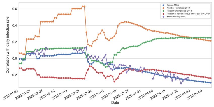
which use Google data to “chart movement trends         2    Data
over time by geography, across different categories
                                                        Twitter offers several ways in which a user can
of places such as retail and recreation, groceries
                                                        indicate their location. If a user is tweeting from
and pharmacies, parks, transit stations, workplaces,
                                                        a GPS enabled device, they can attach their exact
and residential” (Google, 2020). The Unacast “So-
                                                        coordinate to that tweet. Twitter may then display
cial Distancing Scoreboard” uses data collected
                                                        to the user, and provide in their API, the specific
from 127 million monthly active users to measure
                                                        place that corresponds to these coordinates. Al-
the implementation of social distancing practices
                                                        ternatively, a user can explicitly select a location,
(Unacast, 2020). Researchers at the Institute for
                                                        which can be a point of interest (coffee shop), a
Disease Modeling have used data from Facebook’s
                                                        neighborhood, a city, state, or country. If the tweet
“Data for Good” program to model the decline in
                                                        is public, this geolocation information is supplied
mobility in the Greater Seattle area and its effect
                                                        with the tweet.
on the spread of COVID-19 (Burstein et al., 2020).
                                                           We used the Twitter streaming API1 to download
Using cell phone data, the New York Times com-
                                                        tweets based on location. We used a bounding box
pleted an analysis that showed that stay-at-home
                                                        that covered the entire United States, including ter-
orders dramatically reduced travel, but that states
                                                        ritories. We used data from this collection starting
that have waited to enact such orders have contin-
                                                        on January 1, 2019 and ending on April 27, 2020.
ued to travel widely (Glanz et al., 2020). These
                                                        In total, this included 3,768,959 Twitter users and
efforts provide new and important opportunities to
                                                        469,669,925 tweets in United States.
study social distancing in real-time.
   We present the Twitter Social Mobility Index,        3    Location Data
a measure of social distancing and travel patterns      We process the two types of geolocation informa-
derived from public Twitter data. We use public         tion described in the previous section.
geolocated Twitter data to measure how much a              Coordinates The exact coordinates (lati-
user travels in a given week. We compute a metric       tude/longitude) provided by the user (”coordinates”
based on the standard deviation of a user’s geolo-      field in the Twitter JSON object). About 8% of our
cated tweets each week, and aggregate these data        data included ”coordinates”.
over an entire population to produce a metric for          Place The ”place” field in the Twitter json ob-
the United States as a whole, for individual states     ject indicates a known location in which the tweet
and for some US cities. We find that, taking the        was authored. A place can be a point of interest (a
US as a whole, there has been a dramatic drop in        specific hotel), a neighborhood (”Downtown Jack-
travel in recent weeks, with travel between March       sonville”), a city (”Kokomo, IN”), a state (”Ari-
16 and April 27, 2020 showing the lowest amount         zona”) or a country (”United States”). The place
of travel since January 1, 2019, the start of our       object contains a unique ID, a bounding box, the
dataset. Additionally, we find that travel reductions   country and a name. More information about the
are not uniform across the United States, but vary      location is available from the Twitter GEO API.
from state to state. However, there’s no clear corre-   A place is available with a tweet in either of two
lation between the social mobility and confirmed        conditions. First, Twitter identifies the coordinates
COVID-19 cases at the state level. A key advantage      provided by the user as occurring in a known place.
of our approach is that, unlike other travel and so-    Second, if the user manually selects the place when
cial distancing analyses referenced above, we rely      authoring the tweet.
on entirely public data, enabling others to replicate      Since coordinates give a more precise location,
our findings and explore different aspects of these     we use them instead of place when available. If
data. Additionally, since Twitter contains user gen-    we only have a place, we assume that the user is
erated content in addition to location information,     in the center of the place, as given by the place’s
future analyses can correlate attitudes, beliefs, and   bounding box.
behaviors with changes in social mobility.                 For points of interest and neighborhoods, Twit-
  Our findings are presented on http://                 ter only provides the country in the associated
socialmobility.covid19dataresources.org                 metadata. While in some cases the city can be
and we will continue to update our analysis during          1
                                                              https://developer.twitter.com/en/docs/tweets/filter-
the pandemic.                                           realtime/overview/statuses-filter
parsed from the name, and the state inferred, we user based on their centroid location for all time in
opted to exclude these places from our analysis for our collection.
states. The full location details can be obtained We compute the social mobility index for each
from querying the Twitter API, but the magnitude day and week between January 1, 2019 and April
of data in our analysis made this too time consum- 27, 2020. We select the date of March 16, 2020 as
ing. This excluded about 1.8% of our data. the start of social distancing on the national level,
We include an analysis of the 50 most populous though individual states have implemented prac-
United States cites. For this analysis, we included tices at different times. Therefore, we divide the
points of interest that had the city name in their data into two time periods: before social distancing
names, e.g. ”New York City Center”. Specifi- (January 1, 2019 - March 15, 2020) and after social
cally for New York City, we include places that distancing (March 16th, 2020 - April 27, 2020).
corresponded to each of the five New York City We then compute the group level reduction in
boroughs (Brooklyn, Manhattan, Queens, Staten social mobility by considering average values as
Island, The Bronx). follows:
In summary, for each geolocated tweet we have
an associated latitude and longitude. mobility after social distancing
Mobility Reduction = 1− .
mobility before social distancing
4 Computing Mobility (1)
We define the Twitter Social Mobility Index as fol- We also compute the reduction for each user and
lows. For each user, we collect all locations (coordi- then track the median value, number of users active
nates) in a one week period, where a week starts on in both periods, and proportion of active users that
Monday and ends the following Sunday. We com- completely reduce their mobility. We also conduct
pute the centroid of all of the the coordinates and a similar analysis for seasonal effects by comparing
consider this the “home” location for the user for mobility after social distancing and mobility during
that week. We then measure the distance between same period in 2019.
each location and the centroid for that week. For To handle sparse data issues in our dataset, we
distance, we measure the geodesic distance in kilo- exclude (1) users with less than 3 geolocated tweets
meters between two adjacent records using geopy2 . overall, and (2) a weekly record for a user if that
After collecting the distances we measure the stan- user has less than 2 geolocated tweets in that week.
dard deviation of these distances. In summary, this Additionally, due to data loss in our data collec-
measure reflects the area and regularity of travel tion process we remove two weeks with far less
for a user, rather than the raw distance traveled. data than other time periods by taking a 99.75%
Therefore, a user who takes a long trip with a small confidence limit on number of users and records.
number of checkins would have a larger social mo-
bility measure than a user with many checkins who 5 Results
traveled in a small area. As the measure is sensitive
Social Mobility Index Table 2 shows the Twit-
to the number of checkins, it would reflect when
ter Social Mobility Index measured in kilometers
people has less checkins during the pandemic.
for every state and territory in United States, and
We aggregate the results by week by taking the
United States as a whole. City results appear in
mean measure of all users in a given geographic
Table 3. We also include the rank of location by
area. We also present results for a 7-day moving
the group level reduction.
average aggregation as a measure of daily move-
A few observations. The overall drop in mobility
ment. We record the variance of these measures to
across the United States was large: 61.83%. Fig-
study the travel variance in the population, which
ure 1 shows the weekly social mobility index for
will indicate if travel is reduced overall but not for
the United States for the entire time period of our
some users.
dataset. The figure reflects a massive drop in mo-
We produce aggregate scores by geographic area
bility starting in March, with the four most recent
for the United State as a whole, for each US state
weeks the lowest on record in our dataset. Second,
and territory, and for the 50 most populous cities
every US state and territory saw a drop in mobility,
in the US. We determine the geographic area of a
ranging from 38.54% to 76.80% travel compared
2
https://github.com/geopy/geopy to numbers before March 16, 2020. However, theFigure 1: Mean social mobility index (KM) in United States from January 1, 2019 to April 27, 2020. Weeks with missing data are excluded from the figure. variance by state was high. States that were early week March 16 - 22, 2020 and 22.64% in the fol- adopters of social distancing practices are ranked lowing week. We compute a moving-average of highly on the reduction in travel: e.g. Washing- daily mobility data, and use an offline change point ton (3) and Maryland (9). In contrast, the eight detection method (Truong et al., 2020) on this trend. states that do not have state wide orders as of the 62.26% of the change points in 2020 are after the start of April (Zeleny, 2020) rank poorly: Arkansas national announcement date but before the dates (45), Iowa (37), Nebraska (35), North Dakota (22), when individual state policies were enacted. This South Carolina (38), South Dakota (46), Oklahoma suggest that the national announcement had the (50), Utah (14), Wyoming (53). We observe similar largest effect as compared to state policies, a simi- trends in the city analysis, but the median users in lar finding to the cell-phone-based mobility analy- these cities have a larger mobility reduction than sis of four large cities (Lasry et al., 2020). We also the ones in the states. observe that, among 40 states that have announced Besides the group level mobility reduction (Eq. Stay at Home policy, 92.5% of the states have a 4), we also examine the distribution of user level more stationary daily mobility time series before reduction. We only consider users that have at least the policy-announced date, compared to the mo- two checkins in both periods, leading to a subgroup bility time series over all time, suggesting a rapid of all the users in the dataset for the reduction dis- mobility change during pandemic. tribution. The median values for the reduction dis- Finally, Figure 2 shows a box-plot of the mo- tribution is close to 100% for most states. The me- bility variance across all users in a given time pe- dian values for seasonal reduction are all smaller, riod. The distribution is long-tailed with a lot zeros, but still suggest that people substantially reduce so we take the log of 1 plus each mobility index. their mobility during the pandemic. Moreover, in While mobility is reduced in general, some users the United States, 40% of the 818,213 active users are still showing a lot of movement, suggesting completely reduced their mobility, i.e., mobility that social distancing is not being uniformly prac- reduction of 100%. In contrast, the same period in ticed. These results clearly demonstrate that our 2019 saw a 31% reduction among 286,217 active metric can track drops in travel, suggesting that it users. can be used as part of ongoing pandemic response The White House announced “Slow the Spread” planning. guidelines for persons to take action to reduce the spread of COVID-19 on March 16, 2020. 49.06% Correlation What are some of the factors that of the states had their largest mobility drop in the may help explain our Twitter Social Mobility In-
Policy Correlation
State of emergency 0.2587
Date banned visitors to nursing homes 0.1510
Stay at home/ shelter in place 0.1507
Froze evictions 0.1411
Closed non-essential businesses 0.1359
Closed gyms 0.0765
Closed movie theaters 0.0737
Closed day cares 0.0563
Closed restaurants except take out 0.0341
Date closed K-12 schools -0.0821
Table 1: Pearson correlation between cumulative con-
firmed COVID-19 cases at May 10, 2020 and policy
Figure 2: User distribution of mean social mobility release date at each state.
index (KM) before/after social distancing in United
States.
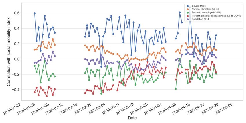
We conduct a similar correlation analysis be-
tween each data source and the social mobility in-
dex? How well does the index track COVID-19 dex, shown in Figure 4. As expected, Geographical
cases compared to other relevant factors? We an- state size has the highest positive correlation. We
alyze our data using a correlation analysis. We also observe that the number of people at risk for
compute daily infection rate by dividing the num- serious illness due to COVID-19 has negative cor-
ber of new confirmed COVID-19 cases in each US relation at the early stage of the pandemic.
state3 by the population of the state. We compare Table 1 investigates the effect of various restric-
the daily infection rate with social mobility index tion policies on confirmed cases by running a sim-
and the following trends (Raifman et al., 2020). ilar correlation analysis on cumulative confirmed
cases for each state on May 10, 2020. The policy
• The size of the state in square miles. types follow the data from (Raifman et al., 2020).
We use the time difference (in days) between May
• The number of homeless individuals (2019). 10, 2020 and policy-released date as the input for
the analysis, and assign a negative value (-1000) for
• The unemployment rate (2018)
states that haven’t announced the policy. The factor
• The percentage of the population at risk for with the highest correlation to the social mobility
serious illness due to COVID-19. index is the declaration of a state of emergency,
which is the broadest type of policy.
For each day we compute the correlation between
the daily infection rate and the above data by state. 6 Related Work
Figure 3 shows the correlation by day. We adopt There is a long line of work on geolocation predic-
infection rate because raw confirmed cases is not tion for Twitter, which requires inferring a location
as informative as the population has the highest for a specific tweet or user (Dredze et al., 2013;
correlation. However, the most significant factor in Zheng et al., 2018; Han et al., 2014; Pavalanathan
the early stage are still population related factors, and Eisenstein, 2015). This includes work on pat-
i.e., number of homeless. We don’t see signifi- terns and trends in Twitter geotagged data (Dredze
cant correlations with other factors including the et al., 2016c). While most of this work focused on
social mobility index. Starting from mid-March, a user, and thus is not suitable for tracking a user’s
we observe trends that unemployment rate, size of movements, there may be opportunities to combine
the state and social mobility index have increas- these methods with our approach.
ing correlation but still not significant enough (the
There have been many studies that have ana-
absolute correlation values < 0.5). The fluctua-
lyzed Twitter geolocation data to study population
tion in the middle is when states started to report
movements. Hawelka et al. (2014) demonstrated a
confirmed cases.
method for computing global travel patterns from
3
https://github.com/CSSEGISandData/COVID-19 Twitter, and Dredze et al. (2016b) adapted thisFigure 3: Pearson correlation between daily COVID-19 infection rates and various factors at state level.
Figure 4: Pearson correlation between social mobility index and various factors at state level.
method to support efforts in combating the Zika 7 Conclusion
epidemic.
We presented the Twitter Social Mobility Index, a
measure of social mobility based on public Twitter
geolocated tweets. Our analysis shows that overall
Several studies have used human mobility pat- in the United States there has been a large drop
terns from Twitter data (Jurdak et al., 2015; Huang in mobility. However, the drop is inconsistent and
and Wong, 2015; Birkin et al., 2014; Hasan et al., varies significantly by state. It appears that states
2013). These studies have included analyses of that were early adopters of social distancing prac-
urban mobility patterns (Luo et al., 2016; Soliman tices have more significant drops than states that
et al., 2017; Kurkcu et al., 2016). Finally, some of have not yet implemented these practices.
these analyses have considered mobility patterns Our work on this data is ongoing, and there are
around mass events (Steiger et al., 2015). several directions that warrant further study. First,as states begin to reopen, and some states main- Mark Dredze, Michael J Paul, Shane Bergsma, and
tain restrictions, tracking changes in population Hieu Tran. 2013. Carmen: A twitter geolocation sys-
tem with applications to public health. In Workshops
behaviors will be helpful in making policy deci-
at the Twenty-Seventh AAAI Conference on Artificial
sions. Second, we focused on the United States, Intelligence.
but Twitter data provides sufficient coverage for
many countries to replicate our analysis. Third, for Eli P Fenichel, Carlos Castillo-Chavez, M Graziano
each user in the dataset there exists tweet content, Ceddia, Gerardo Chowell, Paula A Gonzalez Parra,
Graham J Hickling, Garth Holloway, Richard Ho-
that can reflect a user’s attitudes, beliefs and behav- ran, Benjamin Morin, Charles Perrings, et al. 2011.
iors. Studying these together with their mobility Adaptive human behavior in epidemiological mod-
reduction could yield further insights. Our find- els. Proceedings of the National Academy of Sci-
ings are presented on http://socialmobility. ences, 108(15):6306–6311.
covid19dataresources.org and we will con- James Glanz, Benedict Carey, Josh Holder, Derek
tinue to update our analysis during the pandemic. Watkins, Jennifer Valentino-DeVries, Rick Rojas,
and Lauren Leather. 2020. Where America Didn’t
Stay Home Even as the Virus Spread. https:
//www.nytimes.com/interactive/2020/04/
References
02/us/coronavirus-social-distancing.
Alyce S Adams, STEPHEN B Soumerai, Jonathan Lo- html.
mas, and Dennis Ross-Degnan. 1999. Evidence of
self-report bias in assessing adherence to guidelines. Robert J Glass, Laura M Glass, Walter E Beyeler, and
International Journal for Quality in Health Care, H Jason Min. 2006. Targeted social distancing de-
11(3):187–192. signs for pandemic influenza. Emerging infectious
diseases, 12(11):1671.
Mark Birkin, Kirk Harland, Nicolas Malleson, Philip
Cross, and Martin Clarke. 2014. An examination Google. 2020. COVID-19 community mobility
of personal mobility patterns in space and time us- reports. https://www.google.com/covid19/
ing twitter. International Journal of Agricultural mobility/.
and Environmental Information Systems (IJAEIS),
5(3):55–72. Bo Han, Paul Cook, and Timothy Baldwin. 2014. Text-
based twitter user geolocation prediction. Journal of
Artificial Intelligence Research, 49:451–500.
Roy Burstein, Hao Hu, Niket Thakkar, Andrew
Schroeder, Mike Famulare, and Daniel Klein.
Samiul Hasan, Xianyuan Zhan, and Satish V Ukkusuri.
2020. Understanding the impact of covid-19 policy
2013. Understanding urban human activity and mo-
change in the greater seattle area using mobil-
bility patterns using large-scale location-based data
ity data. https://covid.idmod.org/data/
from online social media. In Proceedings of the
Understanding_impact_of_COVID_policy_
2nd ACM SIGKDD international workshop on ur-
change_Seattle.pdf.
ban computing, pages 1–8.
Peter Caley, David J Philp, and Kevin McCracken. Bartosz Hawelka, Izabela Sitko, Euro Beinat, Stanislav
2008. Quantifying social distancing arising from Sobolevsky, Pavlos Kazakopoulos, and Carlo Ratti.
pandemic influenza. Journal of the Royal Society 2014. Geo-located twitter as proxy for global mobil-
Interface, 5(23):631–639. ity patterns. Cartography and Geographic Informa-
tion Science, 41(3):260–271.
Mark Dredze, David A Broniatowski, Michael C Smith,
and Karen M Hilyard. 2016a. Understanding vac- Qunying Huang and David WS Wong. 2015. Model-
cine refusal: why we need social media now. Ameri- ing and visualizing regular human mobility patterns
can journal of preventive medicine, 50(4):550–552. with uncertainty: An example using twitter data. An-
nals of the Association of American Geographers,
Mark Dredze, Manuel Garcı́a-Herranz, Alex Ruther- 105(6):1179–1197.
ford, and Gideon Mann. 2016b. Twitter as a source
of global mobility patterns for social good. In ICML Raja Jurdak, Kun Zhao, Jiajun Liu, Maurice Abou-
Workshop on #Data4Good: Machine Learning in So- Jaoude, Mark Cameron, and David Newth. 2015.
cial Good Applications. Understanding human mobility from twitter. PloS
one, 10(7).
Mark Dredze, Miles Osborne, and Prabhanjan Kam-
badur. 2016c. Geolocation for twitter: Timing mat- Joel K Kelso, George J Milne, and Heath Kelly. 2009.
ters. In Proceedings of the 2016 Conference of the Simulation suggests that rapid activation of social
North American Chapter of the Association for Com- distancing can arrest epidemic development due to
putational Linguistics: Human Language Technolo- a novel strain of influenza. BMC public health,
gies, pages 1064–1069. 9(1):117.Abdullah Kurkcu, K Ozbay, and EF Morgul. 2016. Jeff Zeleny. 2020. Why these 8 Repub-
Evaluating the usability of geo-located twitter as a lican governors are holding out on
tool for human activity and mobility patterns: A case statewide stay-at-home orders. https:
study for nyc. In Transportation Research Board’s //www.cnn.com/2020/04/04/politics/
95th Annual Meeting, pages 1–20. republican-governors-stay-at-home-orders-coronaviru
index.html.
Arielle Lasry, Daniel Kidder, Marisa Hast, Ja-
son Poovey, Gregory Sunshine, Nicole Zviedrite, Xin Zheng, Jialong Han, and Aixin Sun. 2018. A
Faruque Ahmed, and Kathleen A Ethier. 2020. Tim- survey of location prediction on twitter. IEEE
ing of cmmunity mitigation and changes in re- Transactions on Knowledge and Data Engineering,
ported covid-19 and community mobility—four us 30(9):1652–1671.
metropolitan areas, february 26–april 1, 2020.
Feixiong Luo, Guofeng Cao, Kevin Mulligan, and Xi-
ang Li. 2016. Explore spatiotemporal and demo-
graphic characteristics of human mobility via twit-
ter: A case study of chicago. Applied Geography,
70:11–25.
Savi Maharaj and Adam Kleczkowski. 2012. Control-
ling epidemic spread by social distancing: Do it well
or not at all. BMC Public Health, 12(1):679.
Michael J Paul and Mark Dredze. 2017. Social mon-
itoring for public health. Synthesis Lectures on In-
formation Concepts, Retrieval, and Services, 9(5):1–
183.
Umashanthi Pavalanathan and Jacob Eisenstein. 2015.
Confounds and consequences in geotagged twitter
data. arXiv preprint arXiv:1506.02275.
Kiesha Prem, Yang Liu, Timothy W Russell, Adam J
Kucharski, Rosalind M Eggo, Nicholas Davies, Ste-
fan Flasche, Samuel Clifford, Carl AB Pearson,
James D Munday, et al. 2020. The effect of con-
trol strategies to reduce social mixing on outcomes
of the covid-19 epidemic in wuhan, china: a mod-
elling study. The Lancet Public Health.
J Raifman, K Nocka, D Jones, J Bor, S Lipson, J Jay,
and P Chan. 2020. Covid-19 us state policy database.
Boston, MA: Boston University.
Lydia Saad. 2020. Americans step up their so-
cial distancing even further. https://news.
gallup.com/opinion/gallup/298310/
americans-step-social-distancing-even-further.
aspx.
Aiman Soliman, Kiumars Soltani, Junjun Yin, Anand
Padmanabhan, and Shaowen Wang. 2017. Social
sensing of urban land use based on analysis of twitter
users’ mobility patterns. PloS one, 12(7):e0181657.
Enrico Steiger, Timothy Ellersiek, Bernd Resch, and
Alexander Zipf. 2015. Uncovering latent mobility
patterns from twitter during mass events. GI Forum,
1:525–534.
Charles Truong, Laurent Oudre, and Nicolas Vayatis.
2020. Selective review of offline change point de-
tection methods. Signal Processing, 167:107299.
Unacast. 2020. Social distancing scoreboard.
https://www.unacast.com/covid19/
social-distancing-scoreboard.Mobility (KM) User level reduction
location Before distancing After distancing Group level reduction Median reduction Median seasonal reduction Rank
AK 109.76 25.47 76.80% 99.84% 63.73% 1
AL 48.04 22.57 53.03% 84.47% 72.94% 47
AR 50.54 23.15 54.19% 91.87% 76.81% 45
AZ 62.85 23.47 62.66% 93.69% 85.55% 26
CA 78.58 29.60 62.33% 96.65% 91.35% 29
CO 72.23 24.47 66.12% 98.23% 93.37% 12
CT 45.51 14.89 67.28% 96.29% 89.25% 8
DC 77.67 19.74 74.58% 100.00% 97.75% 2
DE 43.63 13.61 68.81% 93.44% 85.08% 7
FL 76.99 32.24 58.13% 92.38% 82.92% 42
GA 65.64 27.11 58.70% 85.26% 78.00% 39
HI 147.61 70.75 52.07% 97.69% 89.21% 51
IA 50.42 20.59 59.17% 95.91% 89.82% 37
ID 70.77 33.36 52.86% 94.12% 78.19% 49
IL 55.59 19.38 65.15% 98.71% 93.01% 16
IN 45.86 17.15 62.60% 97.19% 89.61% 27
KS 65.50 23.19 64.60% 97.03% 81.57% 19
KY 44.67 15.31 65.74% 93.93% 83.42% 13
LA 45.98 19.39 57.83% 86.13% 77.76% 43
MA 58.69 17.64 69.95% 98.83% 93.93% 5
MD 46.10 15.19 67.04% 94.80% 88.67% 9
ME 59.68 22.45 62.38% 93.77% 78.53% 28
MI 56.24 20.96 62.72% 96.84% 90.42% 25
MN 64.01 21.68 66.13% 98.36% 91.34% 11
MO 52.27 20.08 61.59% 95.89% 88.65% 31
MS 50.24 24.36 51.51% 79.09% 69.11% 52
MT 69.93 32.96 52.86% 90.17% 65.58% 48
NC 52.11 19.73 62.14% 94.27% 85.26% 30
ND 65.77 23.65 64.04% 99.71% 97.21% 22
NE 55.11 21.88 60.29% 99.95% 91.40% 35
NH 55.09 19.48 64.64% 96.26% 85.35% 18
NJ 49.27 14.62 70.33% 97.28% 93.41% 4
NM 58.20 24.23 58.37% 95.66% 73.14% 41
NV 80.25 33.19 58.64% 93.42% 85.00% 40
NY 71.17 24.57 65.48% 98.94% 94.20% 15
OH 44.88 15.73 64.95% 94.81% 88.68% 17
OK 52.34 24.69 52.83% 88.38% 76.99% 50
OR 71.12 25.97 63.49% 97.51% 92.68% 24
PA 54.40 19.45 64.24% 97.59% 89.85% 20
PR 44.96 14.94 66.77% 97.26% 90.38% 10
RI 46.80 14.50 69.01% 96.74% 90.55% 6
SC 48.28 19.85 58.88% 86.03% 77.92% 38
SD 68.41 31.52 53.92% 95.91% 86.66% 46
TN 56.77 21.83 61.55% 94.89% 85.89% 32
TX 73.24 28.60 60.95% 93.81% 84.18% 34
UT 68.43 23.62 65.49% 93.56% 91.50% 14
VA 57.37 22.33 61.07% 95.62% 87.51% 33
VI 132.16 47.57 64.00% 98.66% 87.72% 23
VT 56.84 20.33 64.23% 96.35% 86.70% 21
WA 75.34 21.31 71.71% 98.43% 95.72% 3
WI 56.32 22.68 59.74% 96.88% 91.75% 36
WV 46.59 20.02 57.02% 88.95% 82.40% 44
WY 71.64 44.03 38.54% 84.95% 50.90% 53
United States 65.59 25.04 61.83% 95.86% 88.36% -
Table 2: Reduction of mobility for all states and territories in United States and United States. Ranks are based on
group level reduction.Mobility (KM) User level reduction
location Before distancing After distancing Group level reduction Median reduction Median seasonal reduction Rank
New York City 86.37 29.91 65.38% 99.70% 96.69% 27
Los Angeles 103.16 40.86 60.39% 98.69% 93.87% 40
Chicago 64.09 19.87 69.00% 99.96% 94.58% 14
Houston 53.70 21.50 59.96% 97.04% 88.00% 41
Phoenix 60.07 19.12 68.17% 96.32% 91.08% 18
Philadelphia 54.80 17.70 67.71% 99.16% 93.70% 19
San Antonio 45.43 15.93 64.93% 99.00% 91.33% 28
San Diego 79.21 28.19 64.41% 98.67% 92.77% 30
Dallas 63.92 21.85 65.81% 95.48% 89.32% 25
San Jose 60.63 14.82 75.55% 99.88% 97.34% 2
Austin 72.50 22.84 68.50% 99.66% 94.66% 17
Jacksonville 47.06 26.87 42.90% 96.60% 92.92% 50
Fort Worth 51.67 19.68 61.92% 95.33% 85.72% 37
Columbus 44.67 14.73 67.02% 96.91% 93.15% 22
San Francisco 113.77 31.99 71.89% 99.93% 98.94% 8
Charlotte 58.13 20.90 64.04% 96.26% 89.83% 31
Indianapolis 46.50 14.53 68.76% 99.26% 91.85% 15
Seattle 98.92 21.64 78.12% 99.98% 99.06% 1
Denver 81.11 23.08 71.55% 99.05% 96.30% 9
Washington 80.26 22.12 72.43% 99.93% 97.27% 7
Boston 77.58 27.47 64.59% 99.42% 96.40% 29
El Paso 51.10 21.50 57.92% 100.00% 95.97% 44
Detroit 53.94 22.38 58.50% 94.89% 83.68% 43
Nashville 72.83 23.94 67.13% 98.45% 94.88% 21
Portland 78.91 24.81 68.56% 99.45% 96.81% 16
Memphis 48.64 18.41 62.15% 98.65% 86.75% 35
Oklahoma City 46.07 16.78 63.57% 91.34% 75.19% 33
Las Vegas 80.21 35.69 55.50% 94.87% 83.90% 47
Louisville 45.52 12.97 71.51% 94.31% 77.68% 10
Baltimore 45.61 11.66 74.43% 96.10% 89.37% 4
Milwaukee 52.01 22.78 56.19% 97.01% 91.86% 46
Albuquerque 51.04 16.88 66.93% 98.95% 75.81% 23
Tucson 53.58 23.10 56.89% 95.73% 84.48% 45
Fresno 37.39 10.84 71.02% 96.06% 89.20% 11
Mesa 48.77 21.72 55.47% 92.40% 71.33% 48
Sacramento 62.14 25.45 59.05% 94.82% 94.47% 42
Atlanta 87.90 33.39 62.02% 93.50% 86.36% 36
Kansas City 62.93 17.23 72.61% 98.30% 96.54% 6
Colorado Springs 64.82 23.55 63.67% 99.47% 95.66% 32
Miami 114.33 55.77 51.22% 97.55% 88.56% 49
Raleigh 51.62 15.24 70.47% 97.79% 89.51% 12
Omaha 49.99 15.38 69.24% 100.00% 93.72% 13
Long Beach 54.97 20.51 62.70% 93.33% 89.75% 34
Virginia Beach 48.91 18.92 61.33% 96.35% 88.38% 39
Oakland 87.36 22.26 74.52% 98.41% 96.26% 3
Minneapolis 69.67 18.72 73.14% 99.14% 94.21% 5
Tulsa 48.54 18.51 61.85% 99.89% 93.20% 38
Arlington 56.42 18.27 67.62% 97.58% 93.25% 20
Tampa 70.50 23.55 66.59% 94.48% 83.23% 24
New Orleans 55.96 19.18 65.73% 97.00% 88.75% 26
Table 3: Reduction of mobility for top 50 United States cities by population. Ranks are based on group level
reduction.You can also read