Topographic disequilibrium, landscape dynamics and active tectonics: an example from the Bhutan Himalaya - Earth Surface Dynamics
←
→
Page content transcription
If your browser does not render page correctly, please read the page content below
Earth Surf. Dynam., 9, 895–921, 2021
https://doi.org/10.5194/esurf-9-895-2021
© Author(s) 2021. This work is distributed under
the Creative Commons Attribution 4.0 License.

          Topographic disequilibrium, landscape dynamics and
         active tectonics: an example from the Bhutan Himalaya
            Martine Simoes1 , Timothée Sassolas-Serrayet2 , Rodolphe Cattin2 , Romain Le Roux-Mallouf2,a ,
                                       Matthieu Ferry2 , and Dowchu Drukpa3
                   1 Universitéde Paris, Institut de physique du globe de Paris, CNRS, 75005 Paris, France
          2 Géosciences   Montpellier, Université de Montpellier, CNRS, Université des Antilles, Montpellier, France
                                    3 Department of Geology and Mines, Thimphu, Bhutan
                                           a now at: Géolithe, 38920, Crolles, France

                                     Correspondence: Martine Simoes (simoes@ipgp.fr)

                                Received: 3 December 2020 – Discussion started: 18 December 2020
                             Revised: 21 May 2021 – Accepted: 15 June 2021 – Published: 3 August 2021

       Abstract. The quantification of active tectonics from geomorphological and morphometric approaches com-
       monly implies that erosion and tectonics have reached a certain balance. Such equilibrium conditions are how-
       ever rare in nature, as questioned and documented by recent theoretical studies indicating that drainage basins
       may be perpetually re-arranging even though tectonic and climatic conditions remain constant. Here, we doc-
       ument these drainage dynamics in the Bhutan Himalaya, where evidence for out-of-equilibrium morphologies
       have for long been noticed, from major (> 1 km high) river knickpoints and from high-altitude low-relief regions
       in the mountain hinterland. To further characterize these morphologies and their dynamics, we perform field
       observations and a detailed quantitative morphometric analysis using χ plots and Gilbert metrics of drainages
       over various spatial scales, from major Himalayan rivers to their tributaries draining the low-relief regions. We
       first find that the river network is highly dynamic and unstable, with much evidence of divide migration and
       river captures. The landscape response to these dynamics is relatively rapid. Our results do not support the idea
       of a general wave of incision propagating upstream, as expected from most previous interpretations. Also, the
       specific spatial organization in which all major knickpoints and low-relief regions are located along a longitu-
       dinal band in the Bhutan hinterland, whatever their spatial scale and the dimensions of the associated drainage
       basins, calls for a common local supporting mechanism most probably related to active tectonic uplift. From
       there, we discuss possible interpretations of the observed landscape in Bhutan. Our results emphasize the need
       for a precise documentation of landscape dynamics and disequilibrium over various spatial scales as a first step
       in morpho-tectonic studies of active landscapes.

1   Introduction                                                   leads to steady state after a characteristic time that mostly de-
                                                                   pends on the erosional efficiency (e.g., Whipple and Tucker,
The morphology of the Earth’s surface and its evolution in         1999; Willett et al., 2001; Bonnet and Crave, 2003; Whip-
space and time result from the competition and balance be-         ple and Meade, 2004, 2006; Simoes et al., 2010). This con-
tween tectonics and surface processes. The interplay between       cept of steady state and equilibrium between tectonics and
these processes, with erosion followed by transport and de-        erosion provides an effective conceptual framework, com-
position of the produced sediments in subsiding basins, leads      monly used for investigating and quantifying active tectonics
to a continuous dynamic redistribution of masses, eventu-          from geomorphology (e.g., Lavé and Avouac, 2001). How-
ally modulated by climate (e.g., Allen, 2008). In erosive sys-     ever, topographic equilibrium may only be reached at a re-
tems, such as in uplifting and growing mountain ranges, such       gional scale (Willett and Brandon, 2002) and is expected not
physical competition between uplift and erosion theoretically

Published by Copernicus Publications on behalf of the European Geosciences Union.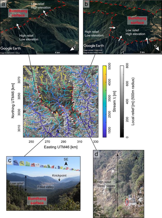
896                                                                         M. Simoes et al.: Landscape dynamics in Bhutan

to be achieved at the more local scale of the drainage net-       ther east, in Bhutan, where evidence for out-of-equilibrium
work even though tectonic and climatic boundary conditions        morphologies has for long been noticed, from the convex to-
remain constant, as illustrated by numerical (e.g., Sassolas-     pographic profile (Fig. 2a and b) and from high-altitude low-
Serrayet et al., 2019) or analog (e.g., Hasbargen and Paola,      relief regions (Fig. 1c) and major knickpoints (Fig. 2c) within
2000) models. The dynamics of the river network are ex-           the mountain hinterland (Duncan et al., 2003; Baillie and
pected to be even more pronounced in natural landscapes           Norbu, 2004; Grujic et al., 2006; Adams et al., 2015, 2016).
for which boundary and forcing conditions vary over time          These morphological features have been interpreted in a vari-
and space. In fact, the formalism used in earlier theoretical     ety of ways, mostly as reflecting either climatic (Grujic et al.,
studies to model erosion is oversimplified as it does not cap-    2006) or tectonic (Baillie and Norbu, 2004; Coutand et al.,
ture the complex 3D dynamic response of drainage basins,          2014; Adams et al., 2016) changes or, in other words, as rep-
in particular through the constant mobility of drainage di-       resenting the landscape transience towards a new equilibrium
vides (e.g., Goren et al., 2014; Willett et al., 2014). An ex-    state. However, recent findings in other contexts question
ample of such landscape dynamics during mountain-building         these interpretations: low-relief landscapes were shown to
lies in the progressive capture of longitudinal drainages by      form possibly dynamically in situ as a response to an increase
steeper transverse rivers, as exemplified in the field (e.g.,     in local base level (e.g., Babault et al., 2007) or to a persistent
Babault et al., 2012), in analog models (Viaplana-Muzas           drainage re-organization even in the case of constant tecton-
et al., 2015), or in the dynamic re-organization of the river     ics and climate (Yang et al., 2015). Finally, despite these ob-
network as a response to tectonic stresses (e.g., Castelltort     servations in Bhutan and the questions they raise, denudation
et al., 2012; Guerit et al., 2018). River captures were also      rates have been regarded as reflecting uplift rates and used to
evidenced in old orogens where topographic equilibrium is         derive the geometry of the underlying main active fault (Le
hypothesized (Prince et al., 2011). This mobility of drainage     Roux-Mallouf et al., 2015) or the timing of interpreted re-
divides leads to a lengthening of the time needed to reach        cent tectonic changes (Adams et al., 2016). Whether or not
theoretical steady state and generates a potential perpetual      these denudation rates are indeed representative of actual up-
transience of landscapes (e.g., Hasbargen and Paola, 2000;        lift rates needs to be probed. Because smaller drainage basins
Yang et al., 2015; Whipple et al., 2017b). It is expected to      are the most inclined to have denudation rates deviating from
generate variations in the sedimentation rates at river outlets   uplift rates in the case of disequilibrium (Sassolas-Serrayet
by modifying the sediment routing system (e.g., Viaplana-         et al., 2019), the answer to this question is intuitively depen-
Muzas et al., 2019) and to elucidate observed large disper-       dent on the size and location of the sampled drainage basins
sions in denudation rates, even in regions that are believed      within the overall drainage system.
to be in quasi-topographic steady state (Willett et al., 2014;       To explore the landscape dynamics of the Bhutan Hi-
Beeson et al., 2017; Sassolas-Serrayet et al., 2019). Interest-   malaya as well as their spatial and temporal characteristics,
ingly, this dispersion in measured denudation rates increases     we hereafter conduct a detailed morphometric analysis of this
most often for smaller drainage basins, further emphasizing       particular field example. We use χ plots (Perron and Royden,
that the concept of steady state is highly scale-dependent as     2013) and Gilbert metrics (Whipple et al., 2017b; Forte and
variations related to the local mobility of drainage divides      Whipple, 2018) for drainages of various dimensions, from
average out at the scale of large river basins (Matmon et al.,    major Himalayan rivers to more local tributary streams drain-
2003; Sassolas-Serrayet et al., 2019).                            ing high-altitude low-relief regions. Our analysis does not
   Here, we propose to further investigate these questions,       reveal any evidence for a general wave of incision migrat-
mostly derived from theoretical studies or in few field cases,    ing upstream the drainage network. Instead, we find ample
by considering the emblematic natural example of the Hi-          evidence for a high instability of the river network at various
malayan range in Bhutan (Fig. 1). Because of their high rates     spatial scales that has not been documented yet, with migrat-
of continental deformation and erosion, the Himalayas have        ing drainage divides and numerous captures. The co-location
for long been an ideal natural case for exploring the interac-    and spatial organization of all geomorphic features along a
tions between tectonics and surface processes, as well as the     longitudinal swath, whatever the considered spatial scale and
associated landscape response (e.g., Beaumont et al., 2001;       the dimensions of the investigated drainage basins, calls for a
Lavé and Avouac, 2001; Burbank et al., 2003; Godard et al.,       common local origin and support of the observed landscape
2004, 2014; Hodges et al., 2004; Thiede et al., 2004, 2005;       dynamics, most probably related to active uplift in the moun-
Grujic et al., 2006; Clift et al., 2010; Adlakha et al., 2013).   tain hinterland as proposed in some earlier studies. Finally,
In particular, the Himalayas of central Nepal have been con-      we discuss the implications of our findings, in particular in
sidered the archetype of a topography equilibrated on aver-       terms of how elevated low-relief regions may have formed
age, from their concave topography and hypsometry (Duncan         and in terms of relative timescales of landscape response to
et al., 2003) or from the observed consistency between de-        network re-organizations.
nudation (Godard et al., 2014), incision (Lavé and Avouac,
2001) and exhumation (e.g., Bollinger et al., 2006) rates over
various spatial and temporal scales. Such is not the case fur-

Earth Surf. Dynam., 9, 895–921, 2021                                                 https://doi.org/10.5194/esurf-9-895-2021
M. Simoes et al.: Landscape dynamics in Bhutan                                                                                             897

Figure 1. Topography, relief and geology of Bhutan. (a) Geological map of Bhutan, after Greenwood et al. (2016). Main tectono-stratigraphic
units are from south to north: the Gangetic Plain (GP), the Siwaliks Hills (SH), the Lesser Himalayan Sequence (LHS) including the Paro
metasediments (PM) in western Bhutan, the Greater Himalayan Sequence (GHS) including some leucogranites, and the Tethyan Sedimentary
Series (TSS). These units are separated by major tectonic contacts, which are from north to south: the Main Frontal Thrust (MFT), the Main
Boundary Thrust (MBT), the Main Central Thrust (MCT), and the South Tibetan Detachment (STD). Locally, some other contacts have been
described such as the Kakhtang Thrust (KT) in north-eastern Bhutan. To the north-west of Bhutan, north of the High Himalayan range, the
Yadong Rift (YR) is part of the southern Tibetan grabens. The extension of the geological map is reported over the shaded topographic map
of (b). (b) Topographic map of Bhutan, from ALOS World 3D – 30 m (AW3D30) DEM data. Main drainage basins are delineated by black
lines, and associated main rivers are color-coded and labeled. Thick colored lines correspond to the main trunk rivers, while thinner lines
indicate main tributaries. Major knickpoints are also reported along trunk and tributary rivers. Dashed rectangles locate the swath profiles
of Fig. 2a and b. Orange and green arrows on the side of these rectangles locate physiographic transitions T2 and T3 as placed in Fig. 2a
and b. Inset denotes the location of the topographic map with respect to regional political borders. (c) Map of local relief, as calculated from
the topography shown in (b), with a moving window of 500 m. Major high-altitude low-relief areas are manually delineated by dashed red
lines. These are from west to east: the Phobjikha (PS), the Bumthang (BS), and the Yarab (YS) surfaces. In western Bhutan, another region
of lower relief is also found in the Bhutan hinterland along the Wang Chhu and Amo Chhu, even though less well defined than the others: the
Wang surface (WS). From west to east, dashed rectangles locate the extension of Figs. S4, 9, 7 and S7 (Figs. S4 and S7 in the Supplement).

https://doi.org/10.5194/esurf-9-895-2021                                                          Earth Surf. Dynam., 9, 895–921, 2021
898 M. Simoes et al.: Landscape dynamics in Bhutan
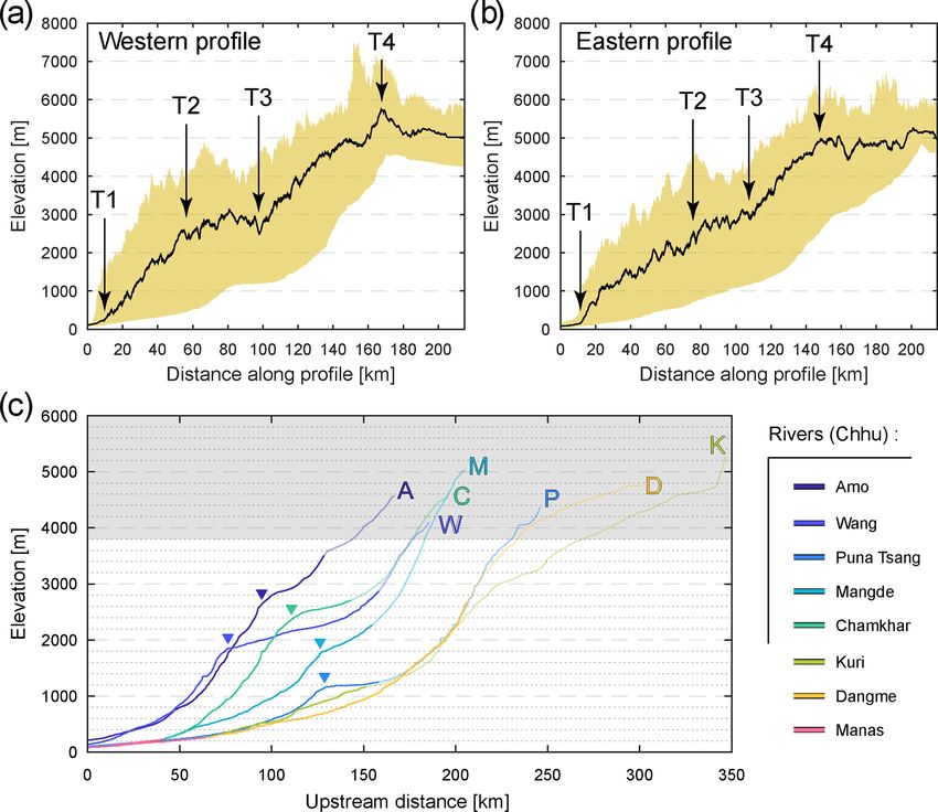
Figure 2. Topographic and longitudinal river profiles. (a, b) Swath topographic profiles across the western (a) and eastern (b) Bhutan
Himalaya over a 100 km wide region, from the Gangetic Plain up to the southern Tibetan Plateau. Location of the swaths is reported in
Fig. 1b. The colored area encompasses the whole range of altitude values, while the black line draws the median altitude across the profiles.
Major physiographic transitions, labeled T1 to T4, are also reported. (c) Longitudinal profiles of major and large rivers in Bhutan, illustrating
the variety of river profiles. Rivers are located on the maps of Fig. 1 and are here color-coded and labeled. Major knickpoints are also pointed
by triangles. Regions with altitudes above 3800 m (grey area) are not to be compared directly to the downstream sections, as these may have
a glacial imprint. Portions of the rivers north of physiographic transition T3 are reported by transparent segments. A: Amo Chhu; M: Mangde
Chhu; C: Chamkhar Chhu; W: Wang Chhu; P: Puna Tsang Chhu; D: Dangme Chhu; K: Kuri Chhu.
2 Geological and geomorphological background deposited on the Indian margin during the Proterozoic and
Paleozoic (e.g., Upreti, 1999; Long et al., 2011b, and refer-
2.1 Geological setting ences therein), and subsequently deformed, metamorphosed
and exhumed since the Mid–Late Miocene, mostly in the
One of the main characteristics of the Himalayan arc is form of duplexes in the mountain hinterland (e.g., Schelling
its structural and tectono-stratigraphic continuity over ca. and Arita, 1991; DeCelles et al., 2001; Huygue et al., 2001;
2500 km (e.g., Gansser, 1964, 1983; McQuarrie et al., 2008). Robinson et al., 2001; Bollinger et al., 2004, 2006; Long
From south to north, and therefore from the Gangetic Plain et al., 2012). Further north, the Greater Himalayan Se-
in the foreland to southern Tibet, major tectonic contacts are quence is thrusted over the Lesser Himalaya along the MCT.
the Main Frontal Thrust (MFT), the Main Boundary Thrust This sequence is constituted of granulites and ortho- and
(MBT), the Main Central Thrust (MCT) and the South Ti- para-gneisses of the former Indian margin, with widespread
betan Detachment (STD). The un-metamorphosed synoro- leucogranites (e.g., Le Fort et al., 1987; Guillot and Le Fort,
genic detrital series of the Siwaliks Group (e.g., Gautam and 1995). The MCT stands as a thick top-to-the-south shear
Rösler, 1999; Coutand et al., 2016) are thrusted over the zone, active by Early to Mid-Miocene (e.g., Tobgay et al.,
Gangetic Plain along the MFT, which stands as the south- 2012, and references therein), and subsequently deformed
ern deformation front of the orogen. The Lesser Himalayan by the duplexes of the Lesser Himalayan series. Finally, the
series are thrusted over the Siwaliks molasses along the Tethyan Sedimentary Sequence is formed of the sedimentary
MBT. These series are formed of metasediments, initially cover of the northern Indian margin (e.g., Liu and Einsele,
Earth Surf. Dynam., 9, 895–921, 2021 https://doi.org/10.5194/esurf-9-895-2021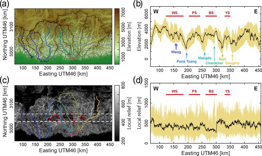
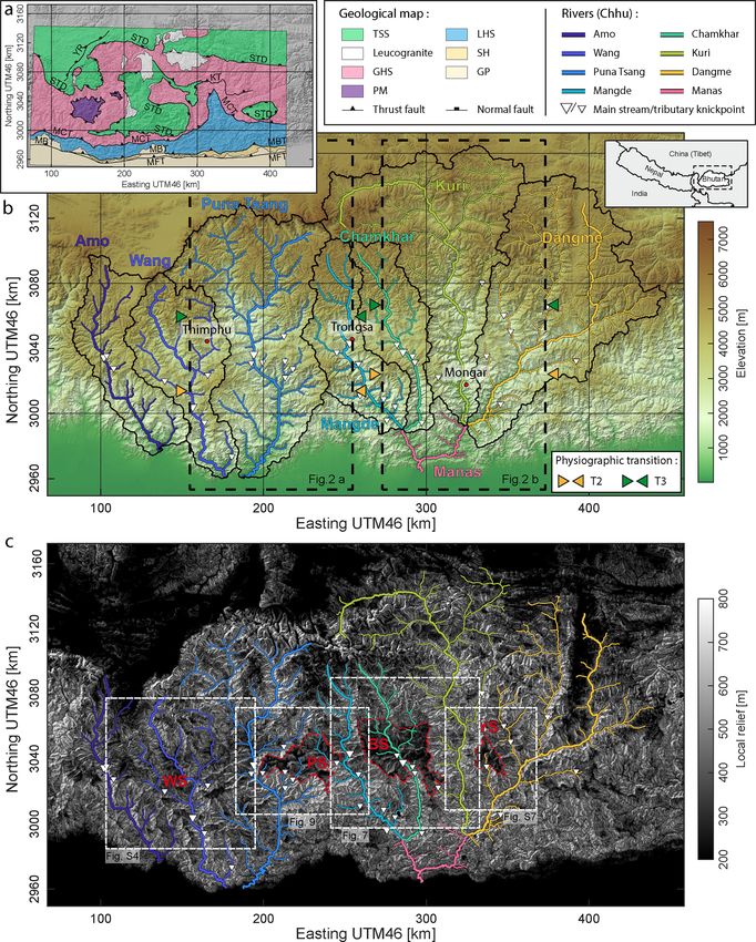
M. Simoes et al.: Landscape dynamics in Bhutan                                                                               899

1994); it is separated from the high-grade Greater Himalayan      surface (e.g., Bilham, 2019, and references therein). Even
rocks by the top-to-the-north normal STD. Except for the un-      though much less investigated, the Bhutan Himalaya is also
metamorphosed Siwaliks, the erodibility of the series present     seismically active (Drukpa et al., 2006). It was struck by
throughout the mountain range is found to be relatively com-      a major historical earthquake in 1714 (e.g., Hetenyi et al.,
parable (Lavé and Avouac, 2001; Adams et al., 2020).              2016), in addition to other past events recently revealed in
   The Bhutan Himalaya obeys this general tectonic and            geomorphological and paleoseismological studies along the
stratigraphic organization observed throughout the Hi-            frontal MFT–MBT thrust system (Berthet et al., 2014; Le
malayan arc (Fig. 1a), even though presenting some pecu-          Roux-Mallouf et al., 2016, 2020).
liarities and specificities (Gansser, 1983; Long et al., 2011a;
Greenwood et al., 2016). In particular, the Greater Himalayan     2.2   Geomorphology of Bhutan: general characteristics
and the Tethyan Sedimentary sequences are here much more
exposed throughout the mountain belt when compared to the         The topography of the Bhutan Himalaya is characterized by
Himalayas of central Nepal where these sequences are only         a convex profile, with four major physiographic transitions,
preserved in the form of individual klippen (e.g., Duncan         hereafter referred to as T1 to T4 from south to north (mod-
et al., 2003). In turn, Lesser Himalayan series mostly crop out   ified after Duncan et al., 2003; Baillie and Norbu, 2004;
along the main topographic mountain front, or within struc-       Adams et al., 2013) (Fig. 2a and b). The first one (T1) corre-
tural windows, such as the Paro window in western Bhutan          sponds to the rise of the mountain topographic front above
(Tobgay et al., 2012) or the larger Lesser Himalayan win-         the Gangetic Plain. Northward, topography increases con-
dow along the Kuri Chhu in eastern Bhutan (Long et al.,           tinuously up to ca. 3000 m on average for the first ca. 70–
2011b) (Fig. 1a). Because of the limited flexural subsidence      80 km (T2), then remains constant on average and high, in-
in the broken foreland of Bhutan (Verma and Mukhopad-             creases again after ca. 100–125 km (T3) and reaches aver-
hyay, 1977; Hammer et al., 2013), most probably related to        age values of ca. 5000 m by ca. 175 km (T4) and northwards
the presence of the Shillong Plateau basement high further        (Fig. 2a and b). Except for T2, these physiographic transi-
south (e.g., Biswas et al., 2007; Clark and Bilham, 2008; Yin     tions are also observed in central Nepal, where the abrupt
et al., 2010), the Siwaliks series is here much less developed    topographic rise between T3 and T4 has been interpreted
than elsewhere along the Himalayan arc (Hirschmiller et al.,      as related to the uplift of the High Himalayan range above
2014), and the MFT is even absent in western Bhutan (Long         the mid-crustal ramp of the MHT (e.g., Lyon-Caen and Mol-
et al., 2011a; Greenwood et al., 2016) (Fig. 1a).                 nar, 1983, 1985; Cattin and Avouac, 2000; Lavé and Avouac,
   All major thrust faults are interpreted to branch off the      2001; Bollinger et al., 2006). This interpretation is also ex-
Main Himalayan Thrust (MHT) at depth, which stands as the         pected to hold in Bhutan, as this elevation ascent coincides
main crustal-scale detachment at the base of the Himalayan        spatially with the location of the recently evidenced mid-
orogenic wedge (e.g., Schelling and Arita, 1991; DeCelles         crustal ramp (Coutand et al., 2014; Marechal et al., 2016;
et al., 2001). Overall, the geometry of the MHT appears quite     Diehl et al., 2017; Singer et al., 2017) – or possibly slightly
simple, with the frontal emerging ramp of the MFT, rooting        deported south of this ramp (Le Roux-Mallouf et al., 2015).
at depth into a wide shallowly north-dipping structural flat,        The abrupt topographic rise from T1 to T2 and the high-
and pursuing northward down to a mid-crustal ramp beneath         altitude region between T2 and T3 are mostly specific to the
the High Himalayan range. This general structure has been         landscape of the Bhutan Himalaya along the Himalayan arc
proposed throughout the Himalayas, in particular in Nepal         (Duncan et al., 2003; Adams et al., 2013). The region be-
(e.g., Lyon-Caen and Molnar, 1983, 1985; Schelling and            tween T2 and T3 is characterized by a locally relatively lower
Arita, 1991; Lavé and Avouac, 2001; Bollinger et al., 2004)       relief (Figs. 1c and 3a–d), in contrast to what is observed fur-
but also more recently suggested in Bhutan, as imaged from        ther south from T1 to T2 (Fig. 3e and f) but also further north
geophysics (Diehl et al., 2017; Singer et al., 2017), or ev-      from T3 to T4 where high-elevation crests are flanked by
idenced from the modeling of interseismic strain (Marechal        deep gorges (Duncan et al., 2003; Baillie and Norbu, 2004;
et al., 2016), thermochronological data (Coutand et al., 2014)    Grujic et al., 2006; Adams et al., 2015, 2016) (Fig. 1). More
or denudation rates (Le Roux-Mallouf et al., 2015). In the        precisely, these lower-relief regions may correspond either
details, the flat structure connecting both the frontal and the   to high-elevation regions around low-relief alluvial valleys
mid-crustal ramps could be locally more complex with sec-         drained by major rivers (e.g., the Wang and Bumthang re-
ondary ramps (e.g., DeCelles et al., 2001; McQuarrie et al.,      gions traversed by the Wang Chhu and Chamkhar Chhu, re-
2008; Adams et al., 2016; Hubbard et al., 2016).                  spectively) (Figs. 1c and 3a and b) or to smaller elevated
   The Himalayan range is actively absorbing shortening,          low-relief landscape patches connected to the main drainage
with rates increasing eastwards from ca. 13 to ca. 21 mm yr−1     network through tributary streams (e.g., Phobjikha or Yarab
along the arc (Stevens and Avouac, 2015). Active tecton-          surfaces) (Figs. 1c and 3c and d). These valleys or surfaces
ics are manifested by numerous historical earthquakes all         are characterized by well-developed soils with saprolite hori-
along the Himalayan arc in addition to paleoseismological         zons and locally contain bogs (Baillie et al., 2004; Adams
evidence of major earthquakes rupturing the MHT up to the         et al., 2016). It should be noted that high-elevation low-relief

https://doi.org/10.5194/esurf-9-895-2021                                               Earth Surf. Dynam., 9, 895–921, 2021
900 M. Simoes et al.: Landscape dynamics in Bhutan
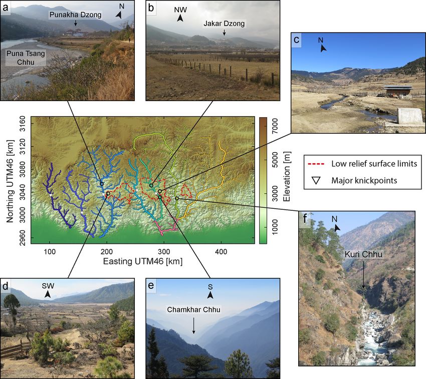
Figure 3. Field pictures representative of the various landscapes in the hinterland of the Bhutan Himalaya. Topographic map in the center
locates field pictures relative to low-relief regions (contoured with red dashed line) and to major knickpoints along rivers (rivers color-
coded as in Figs. 1 and 2). (a) Alluvial plain along the Puna Tsang Chhu, upstream of its major knickpoint. Picture taken near the Dzong
of Punakha. (b) Alluvial plain along the Chamkhar Chhu (Bumthang surface), upstream of its major knickpoint. Picture taken near Jakar.
(c) High-altitude low-relief area of Ura (south-easternmost portion of the Bumthang surface). (d) High-altitude low-relief area of Kotakha
(westernmost portion of the Phobjikha surface). (e) Deep gorge south of the major knickpoint along the Chamkhar Chhu. (f) Canyon along
the Kuri Chhu.
alluvial valleys found along some of the Himalayan rivers Present-day glacial valleys and cirques are mostly re-
(Fig. 3a and b) act as local base levels for upstream erosion. stricted to altitudes higher than ca. 4200 m (Iwata et al.,
Major rivers in Bhutan have their sources along the south- 2002) and are generally located either near T2 or mostly
ern flank of the High Himalayan peaks, except for the trans- north of T3. Glaciers likely advanced and expanded to al-
Himalayan Kuri Chhu and Dangme Chhu to the east, and to titudes of ca. 3800 m during the Holocene and Pleistocene
some extent the Amo Chhu to the west, whose headwaters are (Iwata et al., 2002; Meyer et al., 2009). There is no evidence
located within southern Tibet. These rivers are characterized for glacial imprint on the high-altitude low-relief landscapes
by a variety of profiles (Baillie and Norbu, 2004), but most investigated here, except locally along some of the southern
of them have significant knickpoints, in some cases of the edges of low-relief areas where altitudes reach ca. 4000 m
order of – or higher than – ca. 1 km (Fig. 2c). These knick- (Adams et al., 2016).
points occur at the head of gorges flowing through low-relief
landscapes or immediately downstream of them (Baillie and
Norbu, 2004; Adams et al., 2016) (Figs. 1 and 3e). They sep- 2.3 Geomorphology of Bhutan: previous interpretations
arate rivers in two main segments (Fig. 2c): river profiles are By comparing the morphology and geology of these two
steep downstream of these knickpoints, while upstream river regions of the Himalaya, Duncan et al. (2003) proposed
portions have alluvial fills (Fig. 3a and b) and are located in that topographic and morphologic differences between cen-
the low-relief portions of the mountain range, north of T2. tral Nepal and Bhutan could be related to an along-strike
tectonic segmentation of the Himalayan range and to the
Earth Surf. Dynam., 9, 895–921, 2021 https://doi.org/10.5194/esurf-9-895-2021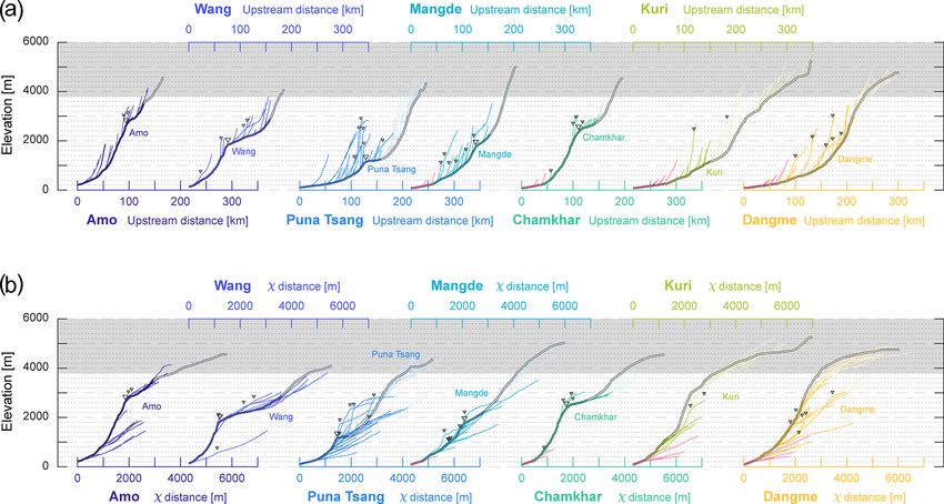
M. Simoes et al.: Landscape dynamics in Bhutan                                                                                  901

associated variable balance between uplift and erosion, in         laterally variable uplift should produce a significant along-
which the timing of large-scale deformation and uplift would       strike variability in exhumation rates, a pattern not seen in
be younger in Bhutan. This interpretation of a less mature         thermochronological data (Grujic et al., 2006; Coutand et al.,
landscape would be supported by the extensive exposure of          2014; Adams et al., 2015). Indeed, most significant variations
Great Himalayan and Tethyan sequences in Bhutan (e.g.,             in exhumation rates are across-strike and not along-strike and
Gansser, 1983; Long et al., 2011a; Greenwood et al., 2016)         should relate to cross-sectional changes in the geometry of
(Fig. 1a), which contrasts with the klippen of central Nepal       the underlying Main Himalayan Thrust (Coutand et al., 2014;
(e.g., Gansser, 1964; Schelling and Arita, 1991; DeCelles          Le Roux-Mallouf et al., 2015).
et al., 2001; Bollinger et al., 2004). Lateral variations in the       More recently, Adams et al. (2015) found that the de-
timing of major fault systems along the Himalayan arc can-         crease in exhumation rates since 4–6 Ma retrieved from ther-
not be excluded, such as for the Main Central Thrust by the        mochronology is observed everywhere in Bhutan, within or
Early to Mid-Miocene (e.g., Tobgay et al., 2012, and refer-        outside a supposed rain shadow, and proposed that it reflects
ences therein) or for the exhumation of the Lesser Himalayan       a southward transfer of deformation towards the Shillong
sequences since the Late Miocene (e.g., Huygue et al., 2001;       Plateau. Morphological characteristics in Bhutan are here
Robinson et al., 2001; Bollinger et al., 2006; Long et al.,        interpreted as a recent local rejuvenation of the landscape
2012, and references therein). However, such interpretation        related to uplift in the mountain hinterland that would not
would first require that the large-scale landscape response        have yet produced sufficient exhumation to be recorded in
time be much greater than what could be justifiable given the      cooling ages. Based on the observation that large rivers are
regional high erosion rates (e.g., Lavé and Avouac, 2001).         over-steepened between physiographic transitions T1 and T2
Also, in this case, erosion rates in Bhutan would be expected      (Fig. 2c) and that most of these rivers develop alluvial plains
to have increased in recent geological times, as a response        upstream of T2 (Fig. 3a and b), these authors proposed that
to balance uplift. However, thermochronological data rather        major convex knickpoints and upstream low-relief regions
suggest a general decrease in exhumation rates over the last       around alluvial valleys are the geomorphic response to the
4–6 Myr (Grujic et al., 2006; Coutand et al., 2014; Adams          uplift related to a local blind duplex in the Bhutan hinter-
et al., 2015).                                                     land (Adams et al., 2016). This interpretation also relies on
   This general decrease in exhumation rates since Late            the similarity between these observations and the results of
Miocene –Early Pliocene has been invoked by Grujic                 a numerical landscape evolution model (after Tucker et al.,
et al. (2006) to be related to the rain shadow generated by        2001) in which rivers adjust to higher uplift rates in the hin-
the coeval topographic rise of the Shillong Plateau further        terland of a mountain range by aggrading upstream of con-
south in the foreland of Bhutan (e.g., Biswas et al., 2007;        vex knickpoints. Major knickpoints are interpreted by Adams
Clark and Bilham, 2008; Govin et al., 2018; Rosenkranz             et al. (2016) as migrating upstream and upwards, and while
et al., 2018, and references therein). Such rain shadow would      so as removing packages of fill deposits in the upstream al-
have led to lower erosion rates and from there to locally in-      luvial valleys. Within this framework, low-relief regions are
creased relief and elevation by modifying the balance be-          interpreted as remnants of formerly incising valleys that were
tween uplift and erosion. Following this idea, high-altitude       filled in situ with sediments while locally uplifted. From
low-relief regions in Bhutan would be relict landscapes of         there, they are used to derive the amount of uplift with re-
prior wetter conditions. However, as noticed by Baillie and        spect to a theoretical initial river profile and the timing of the
Norbu (2004), the rain shadow by the Shillong Plateau is rel-      tectonic perturbation (Adams et al., 2016). Using denuda-
ative as climatic conditions are everywhere wet and tropi-         tion rates measured from in situ produced cosmogenic iso-
cal in Bhutan (Bookhagen and Burbank, 2006). Some vari-            topes in river sands, within and outside the low-relief areas,
ations exist along the foothills, with modern precipitation        Adams et al. (2016) suggest that this rejuvenation is ca. 0.8–
rates peaking to more than 6 m yr−1 on average in between          1 Myr old. Even though the idea of localized uplift over a
physiographic transitions T1 and T2, but climatic conditions       blind ramp is seducing, some details in their interpretation
are then relatively constant northward within the range inte-      need further investigation. Indeed, given the variety of river
rior (north of T2). Also, low-relief regions are mostly found      profiles in Bhutan (Fig. 2c), the choice of the river impacts
within the western half of Bhutan (Fig. 1c), where the Shil-       the amount of uplift derived by comparing the present pro-
long rain shadow is supposedly lowest or inexistent accord-        file with a theoretical one. Also, using differential denuda-
ing to Grujic et al. (2006).                                       tion rates to determine the timing of uplift implies that these
   In addition to these general observations on the overall to-    are representative of uplift rates, an assertion that may not
pography or the presence of low-relief areas in the range inte-    be valid in a setting where the landscape is inevitably out of
rior, Baillie and Norbu (2004) noticed the variety of river pro-   equilibrium (e.g., Sassolas-Serrayet et al., 2019).
files (Fig. 2c), despite overall similar climatic and lithologic       Previous interpretations have therefore attributed the
conditions along Bhutan and from there suggested that these        specificities of the morphology of the Bhutan Himalaya (by
morphologies be mostly related to lateral differential tecton-     contrast to that of central Nepal), to changes in either cli-
ics, accommodated by north–south faulting. However, such           matic or tectonic boundary conditions. They rely on the idea

https://doi.org/10.5194/esurf-9-895-2021                                                 Earth Surf. Dynam., 9, 895–921, 2021
902                                                                         M. Simoes et al.: Landscape dynamics in Bhutan

that high-altitude low-relief regions are either uplifted relict   lation map provides the drainage area upstream each pixel of
landscapes or remnants of formerly incising valleys that have      the DEM and from there allows one to choose the network
been filled in situ while uplifted and imply that major knick-     extension by defining a threshold source area. We extract the
points reflect a general transient wave of incision migrating      river network with a minimal drainage area of 50 km2 . This
upstream into the drainage system. These various assertions        systematic extraction avoids the manual ad hoc selection of
on the dynamics of the river network still need, however, to       specific rivers, which could otherwise bias the analysis.
be clearly documented and explored to verify or refine these          We extract the main river systems of the Bhutan Himalaya
interpretations.                                                   upstream of the topographic front (T1). This supposes that
                                                                   the Gangetic plain is taken as the base level of the extracted
                                                                   upstream drainage network. In eastern Bhutan, major river
3     Data and methods
                                                                   confluences occur just upstream the deformation front: in-
Field observations within the hinterland of Bhutan are com-        deed, the Manas Chhu forms downstream of the conflu-
plemented by a morphometric analysis of the landscape dy-          ence of the four trans-Himalayan rivers – Mangde Chhu,
namics, further detailed hereafter. Fieldwork was conducted        Chamkhar Chhu, Kuri Chhu and Dangme Chhu – from west
during two 2-week-long campaigns in January–February               to east, respectively (Fig. 1). In this specific case, we individ-
2015 and in February 2017.                                         ualize these river systems upstream of their confluences to
                                                                   improve the clarity of the figures and to facilitate their com-
                                                                   parison.
3.1     Topography: data and analytical tools                         Once the river network is extracted, we erase small-scale
Our study relies on topographic data obtained from the             topographic noise associated with DEM artifacts along river
ALOS World 3D – 30 m (AW3D30) digital elevation model              paths using the constrained regularized smoothing (CRS) al-
(DEM) provided by the Japanese Aerospace Exploration               gorithm (see Schwanghart and Scherler, 2017, for further de-
Agency. It has been shown that this DEM has the high-              tails). Smoothing parameters are carefully selected by cross-
est precision when compared to other DEMs with equiv-              checking so as to remove erratic noise while keeping real
alent resolution so that it is well suited to the analysis         topographic features such as knickpoints that may be present
of river profiles in high-relief regions (Schwanghart and          along river profiles. Here, we use a smoothness (parameter K
Scherler, 2017). For our analysis, we use the MATLAB-              in CRS algorithm) of 3.5 and a quantile carving (parameter τ
based function library TopoToolbox, which provides essen-          in CRS) between 10 and 90. The use of smoothed river pro-
tial tools for large-scale geomorphological approaches, in-        files allows for an easier extraction of knickpoints. It also
cluding drainage network and watershed extraction, or com-         allows for a more accurate computation of some stream met-
putation of usual river or topography metrics (Schwanghart         rics (gradient, steepness. . . ).
and Scherler, 2014). For additional information, in particu-
lar on the various algorithms of the library used hereafter,       3.2.2   Extraction of knickpoints
the reader is referred to the TopoToolbox documentation
(https://topotoolbox.wordpress.com, last access: July 2021)        Knickpoints are automatically detected using the “knick-
and to the references provided therein.                            pointfinder” algorithm implemented in TopoToolbox
   Topographic relief is determined as the difference between      (Schwanghart and Scherler, 2014). As for the smoothing
maximum and minimum altitudes in a sliding window of               of river profiles, detection parameters are refined by cross-
500 m radius so as to get a fine resolution on these metrics.      checking, and a tolerance value of 50 is used. The final
Even though we extract morphometric parameters along the           knickpoint list is then manually corrected. We do not con-
whole drainage network, we specifically focus on the region        sider knickpoints above altitudes of 3800 m as these may be
south of the High Himalayan peaks, i.e., south of physio-          mostly due to glacial or post-glacial morphologies. We also
graphic transition T3, where the fluvial network is suppos-        manually remove doubtful minor knickpoints most probably
edly the least affected by a potential glacial imprint (alti-      associated with imperfect local smoothing. This method
tudes < 3800 m) and where morphological features charac-           does obviously not give an exhaustive list of knickpoints
teristic of disequilibrium (major knickpoints, elevated low-       along Bhutanese rivers, but it ensures the retrieval of large
relief regions) have been described.                               knickpoints and of their spatial organization as needed for
                                                                   our study.

3.2     Drainage network analysis
                                                                   3.2.3   Computation of transformed coordinates (χ )
3.2.1    Drainage network extraction and pre-processing
                                                                   The computation of χ-transformed river coordinates has
To extract the hydrographic network, we use the single flow        proved useful for the understanding of landscape and
direction (SFD) algorithm implemented in TopoToolbox,              drainage network dynamics (e.g., Perron and Royden, 2013;
from which an accumulation map is computed. This accumu-           Willett et al., 2014; Yang et al., 2015; Whipple et al., 2017b).

Earth Surf. Dynam., 9, 895–921, 2021                                                  https://doi.org/10.5194/esurf-9-895-2021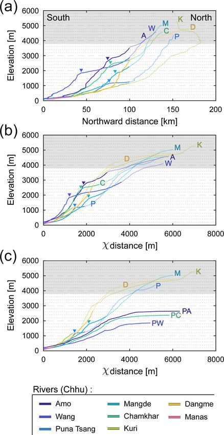
M. Simoes et al.: Landscape dynamics in Bhutan                                                                                               903

Figure 4. Schematic river profiles and metrics expected in the case of equilibrated rivers, of a wave of incision migrating upstream the river
network, or of stream piracy and divide migration. (a) Longitudinal (left) and χ (right) profiles of a main trunk river (dark line) and its
tributaries (grey lines) in the case that these rivers are in equilibrium with external forcing conditions that are constant over the whole area.
The χ profiles of these various rivers are here all linear (constant forcing conditions) and colinear (same forcing conditions), within a certain
variability related to natural conditions (Perron and Royden, 2013). (b) Longitudinal (left) and χ (right) profiles of a main trunk river (dark
line) and its tributaries (grey lines) in the case of the migration of a wave of incision through the river network. Knickpoints are present
along the various streams at variable locations, but their χ profiles are all concordant, within the variability due to natural conditions (Perron
and Royden, 2013). (c) χ profiles expected in the case of migrating divides (left) or river captures (right). Aggressor (or pirate) stream is
represented in red, and the victim in blue. The dark line represents the profile expected for rivers equilibrated with external forcing. Area
gain shifts the χ profiles of aggressor streams to lower χ values, above the equilibrium line. Conversely, area loss shifts the χ profiles of
victim streams to higher χ values, below the equilibrium line. Here, χ profiles are discordant (Willett et al., 2014). (d) Assessment of divide
migration and its direction from the across-divide contrast in χ (Willett et al., 2014) (left) or in Gilbert metrics such as local slope or relief
(Whipple et al., 2017b; Forte and Whipple, 2018) (right).

https://doi.org/10.5194/esurf-9-895-2021                                                           Earth Surf. Dynam., 9, 895–921, 2021
904                                                                         M. Simoes et al.: Landscape dynamics in Bhutan

In this coordinate system, the elevation z at a given position     profiles of main trunk and tributaries that migrate upstream
along the riverbed x depends of the integral quantity χ fol-       following a wave of incision in response to a common change
lowing Eq. (1):                                                    in forcing or boundary conditions are expected to cluster and
                                      1                          be concordant in transformed coordinates (Perron and Roy-
                 U                      n
                                                                   den, 2013) (Fig. 4b). Conversely, migrating knickpoints of
z(x) = z(xb ) +                             χ,              (1)
                KAm0
                                                                   differing origins (e.g., local discrete river captures) will be
                                                                   discordant both in longitudinal and χ profiles. In the case of
with                                                               migrating knickpoints, whether concordant or discordant in
       Zx               m                                        χ coordinates, the river steepness around knickpoints is rep-
                 A0          n
χ=                               dx,                               resentative neither of the actual local uplift rate nor of the
                A(x)                                               erodibility, but rather of the upstream migration of an inci-
       xb
                                                                   sion wave. Spatially fixed knickpoints, as a response to local
where xb locates the channel outlet; A(x) is the drainage area     variations in uplift or erodibility, are expected to be also dis-
upstream of the position x along the channel; A0 is a refer-       cordant in transformed coordinates.
ence scaling area; m and n are constant empirical parameters          Transformed χ plots are also useful to unravel drainage
most often expressed as the m/n ratio. This ratio can be re-       reorganization related to migrating divides and river captures
lated to the reference concavity index θref that describes how     (Willett et al., 2014). A river capture leads to a characteristic
the river gradient evolves along the river profile. Such inte-     χ profile (Willett et al., 2014) (Fig. 4c). Indeed, an abrupt
gral approach is based on the stream power equation of river       increase in drainage area due to a capture shifts the profile
incision (e.g., Howard, 1994; Whipple and Tucker, 1999).           of the pirate stream to lower χ values, i.e., above a theo-
It provides a simple metric for pointing out and analyzing         retical equilibrium profile. Conversely, area loss shifts the
variable forcing conditions or the nature of transient signals     profile of the victim stream to higher χ values, i.e., below
within the river network, by comparing trunk streams and           a theoretical equilibrium profile (Fig. 4c). χ profiles of rivers
their tributaries in profiles corrected for their variable up-     affected by captures are therefore expected to be discordant,
stream drainage areas – and therefore their variable spatial       transiently after the capture and before re-equilibrating to the
scales – (Perron and Royden, 2013) (Fig. 4).                       new boundary conditions. This is also expected for migrating
   The χ plot of an equilibrated concave river system obey-        divides without discrete captures (Yang et al., 2015), unless
ing the stream power equation, with uniform conditions, is a       the response of channels to drainage area changes is faster
straight line along which both main trunk stream and tribu-        than that of divide migration (Whipple et al., 2017b). Such
taries collapse (Fig. 4a). Furthermore, by setting A0 to unity,    signatures of captures or area loss by piracy in transformed
the slope of the χ profile is equal to the channel steep-          coordinates are defined relatively to an equilibrium river pro-
ness Ksn (Perron and Royden, 2013). This metric is linked          file, specified theoretically or in the field from equilibrated
to the uplift rate U and the erodibility coefficient K, by the     trunk or major rivers.
following equation:                                                   It should be noticed that a certain degree of discordance in
                   1                                             transformed χ profiles is acceptable given the variability of
                U    n
                                                                   natural conditions, even in the case of equilibrated rivers or
Ksn =                    .                                  (2)
                K                                                  in the case of rivers responding to a common wave of inci-
   For U and K varying along the profile of the river, steeper     sion (Fig. 4a and b). We choose not to define quantitatively
(gentler) segments in χ profiles relate either to locally higher   what could be taken as an acceptable degree of discordance
(lower) uplift rate or to lower (higher) erodibility. However,     in river profiles as it implies to specify a threshold that is by
any assessment of these parameters from river profiles is not      essence arbitrary. This will not affect our results, and conclu-
direct and straightforward as they depend on parameter n,          sions as major knickpoints in Bhutan are largely dispersed
which is not known a priori (e.g., Mudd et al., 2018). In the      and discordant in χ, amplitude and altitude.
following, we assume that there is no significant variation in        We also use maps of χ along the drainage network to de-
the erosion processes over the study region. Also, we do not       tect potential migrating divides and to assess the direction of
consider a specific value for n and use θref = 0.5 (see Sup-       these migrations. A contrast in the value of χ across a divide
plement, in which the effect of the chosen concavity index is      results in its migration toward the stream with the highest
tested for θref ranging between 0.3 and 0.7). Such assump-         χ (Willett et al., 2014) (Fig. 4d). Recent studies show, how-
tions allow for a relative comparison between the various          ever, that the direction of divide migration interpreted from
parts of the drainage network over our study area.                 a χ analysis is not straightforward and can be biased by the
                                                                   assumed river base level (Whipple et al., 2017b; Forte and
                                                                   Whipple, 2018). Spatially variable tectonic or climatic con-
3.2.4       Assessment of the drainage network dynamics
                                                                   ditions, as well as rock properties, may also maintain χ con-
We use transformed χ profiles to detect and analyze pertur-        trasts across stable divides. To overcome these limitations,
bations within the river network. Knickpoints in longitudinal      we strengthen our analysis of across-divide contrasts by us-

Earth Surf. Dynam., 9, 895–921, 2021                                                  https://doi.org/10.5194/esurf-9-895-2021
M. Simoes et al.: Landscape dynamics in Bhutan 905
Table 1. Drainage areas of large Himalayan rivers in Bhutan, taken
upstream of their outlet at the mountain front or upstream of a major
confluence.
River Drainage area
(km2 )
Amo Chhu 3752
Wang Chhu 4600
Puna Tsang Chhu 9701
Mangde Chhua 3819
Chamkhar Chhua 3174
Kuri Chhub 9652
Dangme Chhub 10 485
a The drainage areas of the Mangde Chhu and
Chamkhar Chhu are here calculated upstream of
their confluence. b The drainage areas of the Kuri
Chhu and Dangme Chhu are here calculated
upstream of their confluence.
ing “Gilbert metrics” associated with contrasts in elevation of
the riverbed, in mean upstream local slope and in mean up-
stream local relief at a given drainage reference area (Whip-
ple et al., 2017b; Forte and Whipple, 2018), taken here as
2 km2 . Migration of the divide is expected to occur towards
the stream with relative higher elevation and conversely with
relative lower local slope or relief (Fig. 4d).
In addition, we infer divide motion by locating morpho-
logical indicators of regressive erosion like beheaded chan-
nels (or wind gaps), from Google Earth satellite imagery or
field observations. These complementary methods enable a
more careful assessment of divide migration direction and
drainage network re-organization. Figure 5. Projected and transformed profiles of major and large
rivers in Bhutan. Rivers are located on the maps of Fig. 1, color-
coded and labeled. Major knickpoints are also pointed by trian-
4 Results gles. Regions with altitudes above 3800 m (grey area) are not to
be compared directly to the downstream sections as these may have
4.1 General observations and definition of the spatial a glacial imprint. Portions of the rivers north of physiographic tran-
scales of investigation sition T3 are reported by transparent segments. (P)A: (proto-)Amo
Chhu; (P)W: (proto-)Wang Chhu; P: Puna Tsang Chhu; M: Mangde
Based on the visual interpretation of longitudinal and χ pro- Chhu; (P)C: (proto-)Chamkhar Chhu; K: Kuri Chhu; D: Dangme
files, we define three profile types for major rivers in Bhutan Chhu. (a) Longitudinal profiles projected along a north–south axis,
(Figs. 2c and 5). First, the Kuri Chhu and Dangme Chhu approximately perpendicular to active tectonic structures and to
in eastern Bhutan are characterized by concave upward pro- structural directions (Fig. 1a). Except for the Wang Chhu, all major
files south of the High Himalayan range (south of physio- knickpoints are located ca. 75–80 km north of the mountain front.
graphic transition T3), with no remarkable major knickpoint. (b) Transformed river profiles, following the formalism of Perron
These rivers correspond to the two largest drainage basins, and Royden (2013). The Gangetic Plain is used as the base level for
with drainage areas > 9000 km2 (Table 1). Second, the Amo all these rivers. χ -transformed profiles are established with a con-
cavity of 0.5 (see Fig. S1 in the Supplement for similar transformed
Chhu, Wang Chhu and Chamkhar Chhu have major knick-
profiles but using other concavity values). (c) Theoretical trans-
points (> 1 km high), located approximately near T2. These formed river profiles of the proto-Wang Chhu, proto-Amo Chhu
knickpoints separate a steep river segment to the south from a and proto-Chamkhar Chhu, compared to the transformed profiles
river segment with lower gradient to the north. More specif- of other large rivers. Profiles of proto-rivers are determined here by
ically, the river portion with lower gradient flows within and removing all the drainage area upstream of the major knickpoint.
across an alluvial plain (Fig. 3b) located in a high-altitude A large portion of these theoretical profiles remains relatively flat
low-relief region (Fig. 1c). These rivers are those among the in transformed coordinates (for χ > ca. 3000 m) as the steepness
major Himalayan rivers of Bhutan with the smallest drainage of these rivers is low near their knickpoint (immediately upstream
basins (drainage areas of < 5000 km2 ) (Figs. 1 and S10 in and downstream), over a limited real distance of a few kilometers at
most.
https://doi.org/10.5194/esurf-9-895-2021 Earth Surf. Dynam., 9, 895–921, 2021906 M. Simoes et al.: Landscape dynamics in Bhutan
the Supplement, Table 1). Third, the Puna Tsang Chhu and and Mangde Chhu are not concordant in transformed coordi-
Mangde Chhu have intermediate characteristics: their longi- nates, with variable χ and most importantly with altitudes
tudinal profile is overall concave upward with a more modest that vary by ca. 600 m.
(< 1 km high) knickpoint near the region of T2, and they flow These observations suggest that major rivers share and
through a limited (Puna Tsang Chhu – Fig. 3a) or inexistent have adjusted overall to similar tectonic and/or climatic forc-
(Mangde Chhu) alluvial plain upstream of this knickpoint. ing conditions in our region of interest, even though these
These major rivers define the local base level for the rivers are located throughout Bhutan.
incision of their tributaries (Fig. 6). Longitudinal profiles
of tributaries exhibit a great variability relative to their 4.3 Large Himalayan rivers draining low-relief alluvial
trunk stream (Fig. 6a). This variability decreases and spe- plains
cific trends emerge when transformed into χ coordinates
(Fig. 6b). On the one hand, most tributaries appear colin- The Chamkhar Chhu, Wang Chhu and Amo Chhu have lon-
ear with their trunk stream in χ plots – at least colinear in gitudinal and χ profiles that are well above those of the for-
χ over comparable spatial regions of the mountain range, in merly discussed major Bhutanese rivers (Figs. 2c and 5b).
particular at the level of their confluence. On the other hand, This is not surprising for longitudinal profiles as these three
some tributaries plot above the trunk stream. These tribu- rivers have more modest drainage areas (Table 1), but this
taries are characterized by a downstream steep channel and pattern remains even in χ coordinates. It should also be
an upstream gentle segment. The gentle segments correspond noticed that the profiles of these rivers are not colinear in
to high-altitude low-relief patches of the landscape (Figs. 1 χ coordinates, with χ values and altitudes of major knick-
and 3c and d). points that vary by ca. 1000 and by ca. 1400 m, respectively
Given the above general observations of major rivers and (Fig. 5b).
of their tributaries, we define various scales of investigation These rivers are also characterized by the mobility of their
of the landscape dynamics in Bhutan. First, we analyze ma- drainage divides, as illustrated in Figs. 7 and S3 in the Sup-
jor trunk rivers draining the Bhutan Himalaya and discuss plement in the case of the Chamkhar Chhu. As intuitively
their diversity. Next, we focus on those showing major knick- expected, the high-altitude low-relief Bumthang region tra-
points and flowing through alluvial plains in high-altitude versed by the Chamkhar Chhu is being laterally aggressed
low-relief regions of the range. We finally analyze the trib- by the tributaries of the deeply incising Mangde Chhu (to
utaries of main trunk rivers, in particular near perched low- the west) and Kuri Chhu (to the east). As a result, the main
relief regions. For each spatial scale, we describe our results drainage divides around this low-relief region are migrating
and present the interpretations that can be directly derived inwards, and the drainage area is locally shrinking (Figs. 7
from them. We recall that we focus hereafter only on the re- and S3). The reverse situation is observed further south,
gions south of physiographic transition T3. downstream of the major knickpoint of the Chamkhar Chhu.
Gilbert metrics suggest that drainage divides are here mi-
grating outwards so that drainage area is locally increasing
4.2 Major Himalayan rivers (Figs. 7 and S3). Similar observations and conclusions are
Here, the longitudinal and χ profiles of the Kuri Chhu, Dan- reached for the Wang Chhu (Fig. S4), even though the situa-
gme Chhu, Puna Tsang Chhu and Mangde Chhu are dis- tion of the Wang Chhu is slightly more complex.
cussed and compared (Figs. 2c and 5). Except for the Mangde Altogether, our results indicate that the Chamkhar Chhu
Chhu, these rivers correspond to the largest drainage basins and possibly the Wang Chhu, flowing through high-altitude
of Bhutan (Table 1). low-relief alluvial plains in the hinterland, have overall dis-
The two easternmost major rivers (Kuri Chhu and Dangme equilibrium characteristics. Their χ profiles, well above the
Chhu) show a very similar long river profile, incising deep regional average defined by the transformed profiles of other
into the mountain range (Fig. 3f) as altitudes of ca. 2000 m major rivers throughout Bhutan (Fig. 5b), are possibly in-
are reached ca. 200 km from their outlet at the Gangetic Plain dicative of a gain of drainage area by large-scale river cap-
(Fig. 2c). This is also the case for the Puna Tsang Chhu, ca. tures (see Fig. 4c; following Willett et al., 2014; Yang et al.,
100–150 km further west in western Bhutan, which only de- 2015). This interpretation is comforted by the fact that the
parts locally from the previous longitudinal profiles by ca. transformed profiles of these rivers get closer to that of other
130 km from the outlet, at the level of its major – but rela- major rivers when corrected for the drainage area upstream of
tively modest (ca. 300–400 m high) – knickpoint. The lon- their major knickpoints (proto-Amo Chhu, proto-Wang Chhu
gitudinal profile of the Mangde Chhu is well above that of and proto-Chamkhar Chhu in Fig. 5c). Additionally, in the
these other major rivers. details, we find evidence for an ongoing dynamic rearrange-
When transformed into χ coordinates, the profiles of these ment of the river network within these large drainage basins,
four rivers compare well and are overall colinear within our with a specific pattern of drainage area loss and expansion on
region of interest south of T3 (Fig. 5b). It should be empha- either side of their major knickpoint.
sized here that the major knickpoints of the Puna Tsang Chhu
Earth Surf. Dynam., 9, 895–921, 2021 https://doi.org/10.5194/esurf-9-895-2021M. Simoes et al.: Landscape dynamics in Bhutan 907
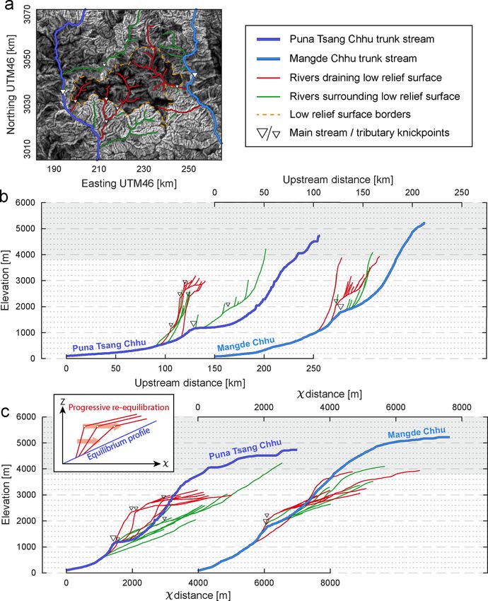
Figure 6. Longitudinal (a – top) and transformed χ (b – bottom) profiles of major rivers of Bhutan and of their tributaries (with drainage
area > 50 km2 ) (location in Fig. 1). Major drainage basins (and the corresponding horizontal axes of their profiles) are color-coded as in
Fig. 1. Trunk streams are reported in bold lines and tributaries in thinner lines. Lighter transparent colors are used for the river portions north
of physiographic transition T3. Major knickpoints are pointed out by triangles. Altitudes above 3800 m are considered aside (grey band)
as rivers may preserve a glacial imprint in these regions. χ -transformed profiles are established with a concavity of 0.5. Other concavities
have been tested and are illustrated in Fig. S2 in the Supplement. For an easier reading of the figure, horizontal axes (distance or χ ) are
alternatively reported below or above the graphs and follow the same color code as that of the rivers they are associated with.
4.4 Low-relief regions captured by secondary streams dinates, with χ values and altitudes that vary by up to ca.
1500 and ca. 1600 m, respectively, in the case of the Puna
At a more local spatial scale, modest high-altitude low-relief Tsang Chhu and its tributaries (Fig. 8c). These streams show
regions (Fig. 3c and d) are connected to the main drainage a peculiar pattern, most obvious in the case of the tributaries
network through secondary streams and tributaries, as for the of the Puna Tsang Chhu: the greater the χ coordinate of the
Phobjikha and Yarab regions (Fig. 1c). knickpoint, the lower the steepness of the stream segment
Starting from the profiles of Fig. 6, we further explore the downstream of the knickpoint, and therefore the closer (in
main features of the drainage network within and around the χ coordinates) the stream profile gets to the regional average
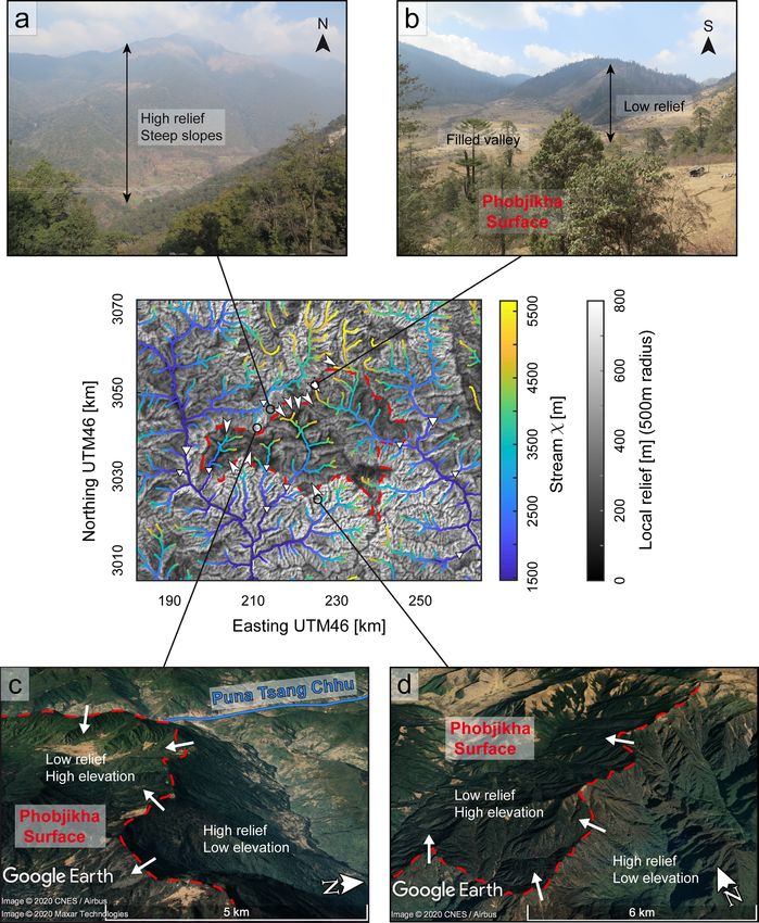
Phobjikha surface using longitudinal and χ profiles of the set by its trunk river (Fig. 8c).
secondary streams, with respect to their main trunk rivers, None of the streams have χ profiles clearly below the re-
the Puna Tsang Chhu and Mangde Chhu (Fig. 8). We here gional average driven by their main trunk channels (Fig. 8c).
follow the approach proposed by Yang et al. (2015) by dif- It is also noteworthy that the χ profiles of the streams ex-
ferentiating streams draining the interior of this low-relief re- ternal to the Phobjikha surface (in green in Fig. 8) remain
gion and those flowing around. External streams (in green in close to – and not above – the regional average imposed by
Fig. 8) have χ profiles mostly colinear with their main trunk their main trunk river (Fig. 8), even though they keep gain-
stream – and more specifically with the local χ profile of ing drainage area by regressive erosion of the low-relief area.
their trunk stream, near their confluence. In contrast, streams Indeed, across-divide contrasts in χ, relief and elevation sug-
draining the Phobjikha low-relief surface (in red in Fig. 8) gest that the Phobjikha region is being regressively eroded all
plot well above the Puna Tsang Chhu or Mangde Chhu in around by surrounding streams (Fig. 9), in particular along
χ coordinates, with a high and low steepness downstream its western divide with the Puna Tsang Chhu as contrasts
and upstream of a major knickpoint, respectively. in χ (Fig. 9) and mostly elevation (Fig. S6 in the Supple-
Interestingly, the streams draining the Phobjikha low- ment) are highest. Contrary to the previous observations on
relief region have major knickpoints that are not concordant low-relief regions drained by the Wang Chhu and Chamkhar
with the major knickpoint of their trunk stream in χ coor- Chhu (Figs. 7, S3 and S4), there is no evidence here for a
https://doi.org/10.5194/esurf-9-895-2021 Earth Surf. Dynam., 9, 895–921, 2021You can also read