Towards a Practical Clustering Analysis over Encrypted Data
←
→
Page content transcription
If your browser does not render page correctly, please read the page content below
Towards a Practical Clustering Analysis
                over Encrypted Data

             Jung Hee Cheon, Duhyeong Kim and Jai Hyun Park

         Department of Mathematical Sciences, Seoul National University
                  {jhcheon,doodoo1204,jhyunp}@snu.ac.kr

      Abstract. Clustering analysis is one of the most significant unsuper-
      vised machine learning tasks, and it is utilized in various fields associated
      with privacy issues including bioinformatics, finance and image process-
      ing. In this paper, we propose a practical solution for privacy-preserving
      clustering analysis based on homomorphic encryption (HE). Our work
      is the first HE solution for the mean-shift clustering algorithm. To re-
      duce the super-linear complexity of the original mean-shift algorithm,
      we adopt a novel random sampling method called dust sampling which
      perfectly fits in HE and achieves the linear complexity. We also substi-
      tute non-polynomial kernels by a new polynomial kernel so that it can
      be efficiently computed in HE.
      The HE implementation of our modified mean-shift clustering algorithm
      based on the approximate HE scheme HEAAN shows prominent perfor-
      mance in terms of speed and accuracy. It takes about 30 minutes with
      99% accuracy over several public datasets with hundreds of data, and
      even for the dataset with 262, 144 data it takes only 82 minutes applying
      SIMD operations in HEAAN. Our results outperform the previously best
      known result (SAC 2018) over 400 times.

      Keywords: clustering, mean-shift, homomorphic encryption, privacy

1   Introduction

For a decade, machine learning has received a lot of attention globally in various
fields due to its strong ability to solve various real world problems. Since many
frequently-used data such as financial data and biomedical data include per-
sonal or sensitive information, privacy is an inevitable issue on machine learning
in such fields. There have been several non-cryptographic approaches for privacy-
preserving machine learning including anonymization, perturbation, randomiza-
tion and condensation [34, 44]; however, these methods commonly accompany
the loss of information which degrades the utility of data.
    On the other hand, Homomorphic Encryption (HE), which allows compu-
tations over encrypted data without any decryption process, is theoretically
one of the most ideal cryptographic primitives to preserve the privacy without
loss of any data information. There have been a number of studies on privacy-
preserving machine learning based on HE, especially for supervised machine
learning tasks such as classification and regression; including logistic regres-
sion [5, 9, 15, 19, 27, 30, 31, 45] and (the prediction phase of) deep neural
networks [6, 25].
     Clustering analysis is one of the most significant unsupervised machine learn-
ing tasks, which aims to split a set of given data into several subgroups, called
clusters, in such a way that data in the same cluster are “similar” in some sense to
each other. As well as classification and regression, clustering is also widely used
in various fields dealing with private information including bioinformatics, image
segmentation, finance, customer behavior analysis and forensics [22, 20, 36].
     Contrary to classification and regression, there are only few works [4, 29] on
privacy-preserving clustering based on HE, and even only one of these works
provides a full HE solution, i.e., the whole procedure is done by HE operations
without any decryption process or trusted third party setting. The main reason
for the slow progress of the research on HE-based clustering is that there are a lot
of HE-unfriendly operations such as division and comparison. Recently, Cheon et
al. [14] proposed efficient HE algorithms for division and comparison of numbers
which are encrypted word-wisely, and this work takes a role of initiating active
research on HE-based clustering.

1.1   This Work
In this paper, we propose a practical solution of privacy-preserving clustering
analysis based on HE. Our solution is the first HE algorithm for mean-shift
clustering which is one of the representative algorithms for clustering analysis.
For given n-dimensional points P1 , P2 , ..., Pp and a function called kernel K :
Rn ×Rn → R≥0 , the mean-shift clustering utilizes the gradient descent algorithm
    Ppfinds local maxima (called modes) of the kernel density estimator F (x) =
which
1
p ·   i=1 K(x, Pi ) where K(x, Pi ) outputs a value close to 0 when x and Pi are
far from each other.
Core Ideas. The main bottlenecks of the original mean-shift algorithm to be
applied on HE are (1) super-linear computational complexity O(p2 ) for each
mean-shift process and (2) non-polynomial operations in kernel which are hard
to be efficiently computed in HE. To overcome these bottlenecks, we suggest
several novel techniques to modify the original mean-shift algorithm into an
HE-friendly form:
 • Rather than mean-shifting every given point, we randomly sample some
   points called dusts and the mean-shift process is done only for the dusts. As
   a result, the computational cost to seek the modes is reduced from O(p2 ) to
   O(d · p) where d is the number of dusts which is much smaller than p.
 • After the mode-seeking phase, one should match given points to the closest
   mode, which we call point-labeling. We suggest a carefully devised algorithm
   for labeling points with the modes which only consists of polynomial opera-
   tions so that it can be implemented by HE efficiently.
                                                                       Γ
 • We propose a new HE-friendly kernel K(x, y) = (1 − ||x − y||2 )2 +1 . The
   most commonly used kernel functions in clustering are Gaussian kernel and

                                         2
Fig. 1. Illustration of the Mean-shift Algorithm
Epanechnikov kernel. However, the derivatives of those functions, which
we should compute for each mean-shift process, are either exponential or
discontinuous. Our new kernel is a simple polynomial which requires only
log(degree) complexity to compute its derivative, and the clustering analy-
sis based on this HE-friendly kernel is very accurate in practice.
Practical Performance: Fast and Accurate. To the best of our knowledge,
the work in [29] has been a unique full HE solution to privacy-preserving clus-
tering so far. While their implementation takes as much as 619 hours for 400 2-
dimensional data, our algorithm takes only about 1.4 hours for the same dataset
which is more than 400 times faster than the previous result. Using a multi-
threading option with 8 threads, the running time is even reduced to half an
hour. The fast and accurate performance of our algorithm implies that the re-
search on HE-based privacy-preserving clustering is approaching to a practical
level.
Why Mean-shift Clustering? K-means clustering is another representative
algorithm for clustering, and many of the previous works on privacy-preserving
clustering exploited the K-means clustering algorithm. However, there are some
critical drawbacks in K-means clustering in the perspective of HE applications.
Firstly, K-means clustering requires a user to pre-determine the exact number of
clusters. However, there is no way to determine the number of clusters when the
only encrypted data are given. Therefore, the data owner should additionally
provide the number of clusters, but determining the exact number of clusters
from a given dataset also requires a costly process even in unencrypted state [41].
Secondly, K-means clustering is generally incapable when the shape of clusters
is non-convex, but the shape of clusters is also non-predictable information from
encrypted data.
31.2 Related Works
In the case of HE-based privacy-preserving clustering, to the best of our knowl-
edge, there has been proposed only a single solution [29] which does not require
any decryption process during the analysis. They transform the K-means clus-
tering algorithm into an HE algorithm based on the HE scheme TFHE [16, 17]
which encrypts data bit-wisely. One of their core idea is to modify the original
K-means clustering algorithm by substituting a homomorphic division of a ci-
phertext, which is very expensive, with a simple constant division. As a result, to
run their modified algorithm with TFHE over 400 2-dimensional data, it takes
about 619 hours (≈ 26 days) on a virtual machine with an Intel i7-3770 processor
with 3.4 GHz without parallelization options. Before this work, there has been
an attempt [4] to perform K-means clustering based on HE with trusted third
party; however, the HE scheme they used [32] was proved to be insecure [46].
Contrary to HE, there have been a number of works [7, 21, 28, 33, 38, 39,
40, 43] on privacy-preserving clustering based on another cryptographic tool
called Multi-party Computation (MPC), which is a protocol between several
parties to jointly compute a function without revealing any information of their
inputs to the others. For more details on MPC-based privacy-preserving cluster-
ing algorithms, we refer the readers to a survey paper written by Meskine and
Nait-Bahloul [35]. MPC is normally known to be much faster than HE; however,
MPC requires online computation of data owners and it yields significantly large
bandwidth. On the other hand, HE computation can be totally done in offline
after encrypted data are sent to a computing service provider. Since data owners
do not need to participate in the computation phase, HE-based solutions can be
regarded to be much more convenient and economic to data owners than MPC.
2 Backgrounds
2.1 Notations
We call each given data of the clustering problem a point. Let n be the dimension
of each point, and P = {P1 , P2 , ..., Pp } be the set of given points where p is the
number of elements in P . We denote the set of dusts, which will be defined in
Section 3, by D = {D1 , D2 , ..., Dd } where d is the number of dusts. There are
several auxiliary parameters for our new algorithms in Section 2 and Section 3:
ζ, t, Γ and T denote the number of iterations for Inv, MinIdx, Kernel and
Mode-seeking, respectively. R denotes the real number field, and R≥0 is a subset
of R which consists of non-negative real numbers. The set Bn (1/2) denotes the
n-dimensional ball of the radius 1/2 with center 0. For an n-dimensional vector
x ∈ Rn , the L2 -norm of x is denoted by ||x||. For a finite set X, x ← U (X) means
that x is sampled uniformly at random from X, and |X| denotes the number of
elements in X. For (row) vectors x ∈ Rn and y ∈ Rm , the concatenation of the
two vectors is denoted by (x||y) ∈ Rn+m . For a positive integer q, [·]q denotes a
residue modulo q in [−q/2, q/2).
42.2 Approximate Homomorphic Encryption HEAAN
For privacy-preserving clustering, we apply an HE scheme called HEAAN pro-
posed by Cheon et al. [13, 12], which supports approximate computation of real
numbers in encrypted state. Efficiency of HEAAN in the real world has been
proved by showing its applications in various fields including machine learn-
ing [15, 30, 31] and cyber-physical systems [11]. After the solution [30] based on
HEAAN won the first place in privacy-preserving genome data analysis compe-
tition called IDash in 2017, all the solutions for the next-year competition which
aimed to develop a privacy-preserving solution for Genome-wide Association
Study (GWAS) computation were constructed based on HEAAN.
In detail, let ct be a HEAAN ciphertext of a plaintext vector m ∈ CN/2 .
Then, the decryption process with a secret key sk is done as
Decsk (ct) = m + e ≈ m
where e is a small error attached to the plaintext vector m. For formal definitions,
let L be a level parameter, and q` := 2` for 1 ≤ ` ≤ L. Let R := Z[X]/(X N + 1)
for a power-of-two N and Rq be a modulo-q quotient ring of R, i.e., Rq := R/qR.
The distribution χkey := HW(h) over Rq outputs a polynomial of {−1, 0, 1}-
coefficients having h number of non-zero coefficients, and χenc and χerr denote
the discrete Gaussian distribution with some prefixed standard deviation. Fi-
nally, [·]q denotes a component-wise modulo q operation on each element of Rq .
Note that those parameters N , L and h satisfying a certain security level can be
determined by Albrecht’s security estimator [3, 2].
A plaintext vector m ∈ Cn/2 is firstly encoded as a polynomial in R by
applying a (field) isomorphism τ from R[X]/(X N + 1) to CN/2 called canonical
embedding. A naive approach is to transform the plaintext vector as τ −1 (m) ∈
R[X]/(X N + 1); however, the naive rounding-off can derive quite a large relative
error on the plaintext. To control the error, we round it off after scaling up by p
bits for some integer p, i.e., b2p · τ −1 (m)e, so that the relative error is reduced.
The full scheme description of HEAAN is as following:
• KeyGen.
- Sample s ← χkey . Set the secret key as sk ← (1, s).
- Sample a ← U (RqL ) and e ← χerr . Set the public key as pk ← (b, a) ∈
Rq2L where b ← [−a · s + e]qL .
- Sample a0 ← U (RqL2 ) and e0 ← χerr . Set the evaluation key as evk ←
(b0 , a0 ) ∈ Rq22 where b0 ← [−a0 s + e0 + qL · s2 ]qL2 .
L
• Encpk (m).
- For a plaintext m = (m0 , ..., mN/2−1 ) in CN/2 and a scaling factor p > 0,
compute a polynomial m ← b2p · τ −1 (m)e ∈ R
- Sample v ← χenc and e0 , e1 ← χerr . Output ct = [v · pk + (m + e0 , e1 )]qL .
• Decsk (ct).
- For a ciphertext ct = (c0 , c1 ) ∈ Rq2` , compute m0 = [c0 + c1 · s]q` .
- Output a plaintext vector m0 = 2−p · τ (m0 ) ∈ CN/2 .
5• Add(ct, ct0 ). For ct, ct0 ∈ Rq2` , output ctadd ← [ct + ct0 ]q` .
• Sub(ct, ct0 ). For ct, ct0 ∈ Rq2` , output ctsub ← [ct − ct0 ]q` .
• Multevk (ct, ct0 ). For ct = (c0 , c1 ), ct0 = (c00 , c01 ) ∈ R2q` , let (d0 , d1 , d2 ) =
−1
(c0 c00 , c0 c01 + c1 c00 , c1 c01 ). Compute ct0mult ← [(d0 , d1 ) + bqL · d2 · evke]q` , and
0
output ctmult ← [b(1/p) · ctmult e]q`−1 .
We omitted the parameters (N, L, h, p) as an input of the above algorithms
for convienience. Let ct1 and ct2 be ciphertexts of plaintext vectors m1 and m2 .
Then, the homomorphic evaluation algorithms Add and Mult satisfy
Decsk (Add(ct1 , ct2 )) ≈ m1 + m2 ,
Decsk (Multevk (ct1 , ct2 )) ≈ m1 m2
where denotes the Hadamard (component-wise) multiplication, i.e., addi-
tion and multiplication can be internally done in a Single Instruction Multi
Data (SIMD) manner even in encrypted state. For more details of the scheme
including the correctness and security analysis, we refer the readers to [13].
To deal with a plaintext vector of the form m ∈ CK having length K ≤ N/2
for some power-of-two divisor K of N/2, HEAAN encrypts m into a ciphertext of
an N/2-dimensional vector (m|| · · · ||m) ∈ CN/2 . This implies that a ciphertext
0
of m ∈ CK can be understood as a ciphertext of (m|| · · · ||m) ∈ CK for powers-
of-two K and K 0 satisfying K ≤ K 0 ≤ N/2 .
Bootstrapping of HEAAN. Since the output ciphertext of a homomorphic
multiplication has a reduced modulus by the scaling factor p compared to the
input ciphertexts, the homomorphic operation should be stopped when the ci-
phertext modulus becomes so small that no more modulus reduction can be done.
In other words, without some additional procedure the HE scheme only supports
polynomial operations with a bounded degree pre-determined by HEAAN pa-
rameters.
A bootstrapping algorithm, of which the concept was firstly proposed by Gen-
try [24], enables us to overcome the limitation on the depth of computation. The
bootstrapping algorithm gets a ciphertext with the lowest modulus ct ∈ Rq21
as an input, and outputs a refreshed ciphertext ct0 ∈ Rq2L0 where L0 is a pre-
determined parameter smaller than L. The important fact is that the bootstrap-
ping preserves the most significant bits of a plaintext, i.e., Decsk (ct) ≈ Decsk (ct0 ).
In 2018, a first bootstrapping algorithm for HEAAN was proposed by Cheon et
al. [12], and later it was improved by several works concurrently [8, 10].
Even though the performance of bootstrapping has been improved by active
studies, the bootstrapping algorithm is still regarded as the most expensive part
of HE. In the case of HEAAN, the performance of bootstrapping depends on the
number of plaintext slots K; roughly the computational complexity is O(log K)
considering SIMD operations of HEAAN.
2.3 Non-polynomial Operations in HEAAN
Since HEAAN basically supports homomorphic addition and multiplication, per-
forming non-polynomial operations in HEAAN is clearly non-trivial. In this sec-
6tion we introduce how to perform the division and a comparison-related oper-
ation called min-index in word-wise HE including HEAAN, which are required
for our mean-shift clustering algorithm. Note that the following methods are
essentially efficient polynomial approximations for the target operations.
Division. The Goldschmidt’s divison algorithm [26] is an approximate algorithm
to compute the inversion of a positive real number in (0, 2), and has been used
in various cryptographic applications [14, 18] to deal with inversion and division
operations through a polynomial evaluation. The algorithm approximates the
inversion of x ∈ (0, 2) by
∞
1 Y ζ−1
2i 2i
Y
= 1 + (1 − x) ≈ 1 + (1 − x)
x i=0 i=0
where ζ is a parameter we choose considering the approximation error. If the
range of an input is (0, m) for large m > 0 which is known, then the Gold-
schmidt’s division algorithm can be easily generalized by simply scaling down
the input into the range (0, 2) and scaling up the output after the whole process.
Algorithm 1 Inv(x; m, ζ)
Input: 0 < x < m, ζ ∈ N
Output: an approximate value of 1/x
1: a0 ← 2 − (2/m) · x
2: b0 ← 1 − (2/m) · x
3: for i ← 0 to ζ − 1 do
4: bi+1 ← b2i
5: ai+1 ← ai · (1 + bi+1 )
6: end for
7: return (2/m) · aζ
Min Index. In [14], Cheon et al. proposed the iterative algorithm MaxIdx to
compute the max-index of an array of positive numbers which can be homomor-
phically computed by HEAAN efficiently. More precisely, for an input vector
x = (x1 , x2 , .., xm ) where xi ∈ (0, 1)
are distinct numbers, then the output of
2t
Pm 2t
the max-index algorithm is a vector xi /( j=1 xj ) for sufficiently large
1≤i≤m
t > 0, whose i-th component is close to 1 if xi is the maximal element, and is
approximately 0 otherwise. If there are several maximal numbers, say x1 , ..., x`
for 1 ≤ ` ≤ m without loss of generality, then the output vector is approximately
(1/`, 1/`, ..., 1/`, 0..., 0).
As a simple application of max-index, one can also compute the min-index
of an array of positive numbers in (0, 1) by running the MaxIdx algorithm for
input (1−x1 , 1−x2 , ..., 1−xm ). The following algorithm describes the min-index
algorithm denoted by MinIdx.
7Algorithm 2 MinIdx((xi )m i=1 ; t, ζ)
Input: (x1 , ..., xm ) ∈ (0, 1)m where ` ≥ 1 elements are minimal, t ∈ N
Output: (y1 , ..., ym ) where yi ≈ 1/` if xi is a minimal element and yi ≈ 0
otherwise;
1: sum ← 0
2: for i ← 1 to m do
3: yi ← 1 − xi
4: for j ← 1 to t do
5: yi ← yi · yi
6: end for
7: sum ← sum + yi
8: end for
9: inv ← Inv(sum; m, ζ)
10: for i ← 1 to m do
t Pm t
11: yi ← yi · inv // yi ' (1 − xi )2 / j=1 (1 − xj )2
12: end for
13: return (y1 , ..., ym )
2.4 Mean-shift Clustering
The mean-shift clustering algorithm is a non-parametric clustering technique
which does not restrict the shape of the clusters and not require prior knowledge
of the number of clusters. The goal of the algorithm is to cluster the given points
by finding the local maxima (called modes) of a density function called Kernel
Density Estimator (KDE), and this process is essentially done by the gradient
descent algorithm. For given n-dimensional points P1 , P2 , ..., Pp and a function
K : Rn × Rn → R≥0 so-called kernel, the KDE map F : Rn → Rn is defined as
p
1 X
F (x) = · K(x, Pi ).
p i=1
The kernel K is defined by a profile k : R → R≥0 as K(x, y) = ck · k(||x − y||2 )
for some constant c > 0. Through a simple computation, one can check that
0 2
i || )·Pi
Pp
∇F (x) is parallel to i=1 Pkp (||x−P 0
0
2 − x where k is the derivative of k.
i=1 k (||x−Pi || )
As a result, the mean-shift process is to update the point x as
p p
!
X k 0 (||x − Pi ||2 ) X k 0 (||x − Pi ||2 )
x←x+ Pp 0 2
· P i − x = Pp 0 2
· Pi ,
i=1 j=1 k (||x − Pj || ) i=1 j=1 k (||x − Pj || )
which is the weighted mean of given points. The most usual choices of the
kernel
function are the Gaussian kernel KG (x, y) = ckG · exp −||x − y||2 /σ 2 and the
Epanechnikov kernel KE (x, y) = ckE · max(0, 1 − ||x − y||2 /σ 2 ) for x, y ∈ Rn
with an appropriate parameter σ > 0 and constants ckG and ckE . Algorithm 3 is
a full description of the original mean-shift clustering algorithm with Gaussian
kernel.
8Algorithm 3 MS-clustering-original(P = {P1 , ..., Pp }, T ; σ)
Input: P1 , P2 , · · · , Pp ∈ Rn , the number of iterations T ∈ N
Output: Label vector M of given points P1 , ...., Pp
1: for i ← 1 to p do
2: M i ← Pi
3: end for
4: for i ← 1 to T do
5: for j ← 1 to p do
6: sum ← 0
7: A ← 0d
8: for k ← 1 to p do
9: a ← exp(−||Pk − Mj ||2 /σ 2 )
10: A ← A + a · Pk
11: sum ← sum + a
12: end for
13: Mj ← (1/sum) · A
14: end for
15: end for
16: return M = (M1 , ..., Mp )
Freedman-Kisilev Mean-shift. A decade ago, Freedman and Kisilev [23] pro-
posed a novel fast mean-shifting algorithm based on the random sampling. As the
first step, for the given set P = {P1 , P2 , ..., Pp } which consists of n-dimensional
points, they randomly choose a subset P 0 ⊂ P of the cardinality p0 . Here the
cardinality p0 is indeed smaller than p but should not be too small so that the
subset P 0 approximately conserves the distribution of the points. For example, if
the random sampling factor p/p0 is too high, then Freedman-Kisilev mean-shift
algorithm shows a quite different result compared to that of the original mean-
shift algorithm. After the random sampling phase, the second step is simply to
run the original mean-shift algorithm on the randomly chosen subset P 0 and
obtain the modes of KDE constructed by P 0 not P . Since only p0 points are used
for mean-shifting process, the computational complexity of this phase is O(p02 ),
not O(p2 ). The last step so-called “map-backwards” is to find the closest point
in Pj0 ∈ P 0 for each point in Pi ∈ P and then output the mode mean-shifted
from Pj0 . The last step takes O(p0 · p) computational complexity which is still
smaller than O(p2 ). Note that the last step map-backwards in Freedman-Kisilev
mean-shift algorithm is not required in the original mean-shift algorithm, since
every point converges to some mode which takes a role of the label.
2.5 Clustering Quality Evaluation Criteria
To evaluate the quality of our clustering analysis results, we bring two measures:
accuracy and silhouette coefficient. The accuracy is measured by comparing the
clustering analysis result and the given true label information. Let Li and C(Pi )
9be the true label and the label obtained by clustering analysis of the point Pi ,
respectively, then the accuracy is calculated as
|{1 ≤ i ≤ p : Li = C(Pi )}|
Accuracy = .
p
Note that the measure is valid only if the number of clusters of the given true
label information equals to that of the clustering analysis result.
The silhouette coefficient [37] is another measure which evaluates the quality
of clustering analysis, which does not require true label information to be given.
Let Q1 ,...,Qk be the clusters of the given dataset P obtained by clustering anal-
ysis. For each point Pi which belongs to the cluster Qki , we first define two
functions A and B as
1 X 1 X
A(Pi ) = · dist(Pi , P` ), B(Pi ) = min · dist(Pi , P` ).
|Qki | − 1 j6=i |Qkj |
P` ∈Qki P` ∈Qkj
`6=i
Then, the silhouette coefficient is defined as
p
1 X B(Pi ) − A(Pi )
SilhCoeff = · ,
p i=1 max(B(Pi ), A(Pi ))
which indicates how well the points are clustered. It is clear that −1 ≤ SilhCoeff ≤
1, and the silhouette coefficient closer to 1 implies the better result of clustering.
3 HE-friendly Modified Mean-shift Clustering
In this section, we introduce several modifications on the mean-shift algorithm
so that the modified algorithm can be efficiently performed by HE. One big
drawback of the original mean-shift algorithm to be implemented by HE is the
evaluation of kernel functions. They usually contain non-polynomial operations,
but these operations cannot cannot easily computed with HE algorithms. To
overcome the problem, we suggest a new HE-friendly kernel function in Sec-
tion 3.1 which is computationally efficient and shows a good performance.
Another big drawback of the original mean-shift algorithm to be implemented
by HE is its high computational cost. The usual mean-shift process classifies data
by seeking modes and mapping points to its corresponding mode at the same
time. This strategy eventually forces us to perform mean-shift process on all data,
so it is computationally inefficient to be implemented by HE which necessarily
accompanies more than hundreds or thousands times of overhead. To address this
issue, we adopt a random sampling method called dust sampling, and separate
the total mean-shift clustering process into two phases: mode-seeking phase and
point-labeling phase. One can check the details on these two phases in Section 3.2
and Section 3.3 respectively, and the full description of our modified mean-shift
clustering algorithm is described in Section 3.4.
103.1 HE-friendly Kernel
As described in Section 2.4, the most popular kernel functions for mean-shift al-
gorithm are Gaussian kernel and Epanechnikov kernel. However, the derivatives
of both kernel functions, which should be computed in the mean-shift cluster-
ing algorithm, are either exponential or discontinuous that cannot be directly
computed with HE.
To overcome those drawbacks, we propose a new HE-friendly kernel function
which is a polynomial. We aim to construct a kernel function that vanishes
rapidly as its input goes far from the origin. Also, we consider about reducing
the number of multiplications during the computation of the kernel as well. For
each x ∈ [0, 1], our new profile k is calculated as following:
2Γ +1
k(x) = (1 − x) . (1)
The degree was set 2Γ + 1 to reduce the computational complexity of the deriva-
tive function k 0 which should be computed for mean-shift. Using this profile, a
new HE-friendly kernel is defined as following: For x, y ∈ Bn (1/2), the kernel
function K based on the profile k is
2Γ +1
K(x, y) = c · 1 − ||x − y||2 (2)
for some constant c > 0. The following algorithm, denoted by Kernel, shows a
very simple computation of k 0 (||x − y||2 ) up to constant −1/(2Γ + 1) which will
be eliminated. If one chooses bigger Γ , the kernel function will decrease more
rapidly, so the mean-shift process will focus more on closer points. Conversely, if
one chooses smaller Γ , the kernel function decreases slowly so that the mean-shift
process references wider area.
Algorithm 4 Kernel(x, y; Γ )
Input: x, y ∈ Bn (1/2), Γ ∈ N
Output: HE-friendly kernel value between A and B
1: a ← 1 − ||x − y||2
2: for i ← 1 to Γ do
3: a ← a2
4: end for
5: return a
Our new kernel function is composed of (Γ + 1) multiplications and one con-
stant addition, while Γ is very small compared to the degree of the kernel poly-
nomial (Γ = log(degree)). Thus, our new kernel function is very HE-friendly. At
the same time, it is non-negative and strictly decreasing, which are core condi-
tions of a kernel function for mean-shift algorithm. Moreover, its rapid decreasing
property provides high performance for mean-shift. The performance of our new
11kernel function is experimentally proved under various datasets (See Section 4).
In unencrypted state, the mean-shift clustering with our kernel shows almost
same performance with that with the Gaussian kernel under same datasets de-
scribed in Section 4.1.
3.2 Mode-seeking Phase
The biggest drawback of the original mean-shift clustering algorithm is its high
time complexity. It requires super-linear operations in the number of data points.
Since HE consumes considerably long time to compute each operation, it is
strongly demanded to modify mean-shift algorithm to practically use it with
HE.
To overcome those drawbacks, we use random sampling to reduce the total
number of operations for each mean-shift process. Instead of performing mean-
shift on every point, we perform the mean-shift process only on selected points
which we shall call dusts. Obviously each mean-shift process references all the
data so that dusts move to some modes of the KDE map. After sufficiently many
iterations, each dust converges to a mode, so we can seek all modes if we selected
enough dusts.
Advantage of the Dust Sampling Method. Our modification has a great
advantage on the number of operations. In the original mean-shift clustering
algorithm, every point shifts its position by referencing all of the other points.
Algorithm 5 Mode-seeking(P = {P1 , ..., Pp }, d, T ; Γ, ζ)
Input: Points P1 , P2 , · · · , Pp ∈ Bn (1/2), the number of dusts d ∈ N, the number
of mean-shift iterations T ∈ N
Output: Mean-shifted dusts Di ∈ Bn (1/2) close to modes for 1 ≤ i ≤ d
1: for i ← 1 to d do
2: Di ← U (P ) // selecting dusts among Pi ’s
3: end for
4: for i ← 1 to T do
5: for j ← 1 to d do
6: sum ← 0
7: A ← 0d
8: for k ← 1 to p do
9: a ← Kernel(Pk , Dj ; Γ )
10: A ← A + a · Pk
11: sum ← sum + a
12: end for Pp k0 (||Dj −Pi ||2 )
13: Dj ← Inv(sum; p, ζ) · A // Dj ← i=1 Pp k0 (||D 2 · Pi
j −P` || )
`=1
14: end for
15: end for
16: return D
12Hence, it needs O(p2 ) operations for each loop where p is the number of given
points. However, in our approach, only selected dusts shift their positions, so
we can complete each mean-shift loop with O(p · d) operations, where d is the
number of selected dusts. This drastically reduces the total number of operations
because we select only few dusts among numerous points.
Even though our approach requires less operations, its performance is accept-
able. Since we exploit the KDE map over all given points, the dusts converge
to modes exactly in the same way to the original mean-shift algorithm. Conse-
quently, we can seek all modes by selecting sufficiently many dusts.
How to Sample Dusts? There are many possible ways to set the initial po-
sition of dusts. We consider two candidates of initializing the dusts. One is to
uniformly select dusts from the space (so that can form a grid ) and the other is
to select dusts among the given points. The first strategy is tempting because it
guarantees high probability to seek all the modes. However, as the dimension of
the data set becomes higher, it requires too many dusts which directly increases
the total time complexity. On the other hand, the second strategy provides sta-
ble performance with less number of dusts even if the dimension and shape of
the data vary. Moreover, it chooses more dusts from the denser regions, so we
can expect that it succeeds in detecting all centers of clusters. Thus, we use the
second strategy, selecting dusts among given points as described in Algorithm 5.
Comparison to Freedman-Kisilev’s Method. At first glance, our approach
looks similar to that of Freedman and Kisilev [23]. Remark that they pick p0
random samples among the data, and run the original mean-shift clustering
algorithm only on the randomly sampled points.
Compared to Freedman-Kisilev mean-shift, the number of selected dusts d in
our mean-shift can be set smaller than the number of randomly sampled points
p0 . While our sampling method use the original KDE itself, Freedman-Kisilev
algorithm use KDE of the selected samples instead of the original KDE. As a
consequence, Freedman and Kisilev have to select substantially many samples
that can preserve the original KDE structure in some sense, while we do not
have such restriction on the number of dusts.
The computational complexity of each mean-shift process in Freedman and
Kisilev’s algorithm is O(p02 ) , while ours is O(d · p). If p0 is large enough so that
d · p < p02 , our mean-shift process requires even less computations. And even if
p0 has been set small enough so that p02 < p · d, the computational complexity
of the map-backwards process in Freedman-Kisilev mean-shift O(p · p0 ) is still
larger than that of point-labeling process in our mean-shift O(p · d) since p0 > d.
More importantly, the less number of selected dusts in our approach has a huge
advantage on HE implementation. Bootstrapping is the most expensive part
in HE, so minimizing the cost of bootstrapping, by reducing the number of
bootstrappings or setting the number of plaintext slots as small as possible, is
very important to optimize HE implementations. Since the mean-shift clustering
algorithm requires very large amount of computations, we have to repeatedly
execute bootstrapping on d dusts in the case of our algorithm and p0 samples in
the case of Freedman-Kisilev. Since d < p0 , the total bootstrapping procedure
13takes much less time in our mean-shift algorithm than the Freedman-Kisilev
mean-shift algorithm.
3.3 Point-labeling Phase
Let us move on to the second phase, point-labeling. After finding all the modes,
we should label each point by mapping it to its closest mode. A naive way to
label a point Pi is as followings:
Cnaive (Pi ) = argmin1≤j≤d dist(Dj , Pi )
where each Di denotes the mean-shifted dust after the mode-seeking phase.
However, the argmin function is very hard to compute in HE, and furthermore
this naive approach would label the points in the same cluster with different
indices. For example, let two dusts D1 and D2 converge to a same mode M
after the mean-shift process, and P1 and P2 are unselected points of which the
closed dusts are D1 and D2 respectively. We expect P1 and P2 to be classified
as a same cluster because both points are close to the same mode M . However,
with the naive way of point-labeling above, Cnaive (P1 ) = 1 does not match with
Cnaive (P2 ) = 2 due to the slight difference between D1 and D2 .
Fortunately, exploiting MinIdx algorithm in Section 2.3 resolves both prob-
lems of the naive approach. Let us define a modified point-labeling function C 0
as
C 0 (Pi ) = MinIdx (||Pi − Dk ||2 )1≤k≤d ; t, ζ .
Since MinIdx algorithm consists of polynomial operations, it can be evaluated by
HE for sure. Moreover, for appropriate parameters t and ζ, MinIdx((x1 , ..., xm ); t, ζ)
outputs a vector close to 21 , 12 , 0, ..., 0 when x1 and x2 are (approximately) min-
imal among xi ’s, rather than (1, 0, ..., 0) or (0, 1, ..., 0). Therefore, in the same
setting to above, we get C 0 (P1 ) ' C 0 (P2 ) ' 21 , 21 , 0, ..., 0 .
However, C 0 cannot be a complete solution when considering the case that a
lot of Di ’s converge to a same mode. Let D1 , ..., D` converged to the same mode
M after the mean-shifting process. Then for a point Pi which is close to the
mode M , it holds that C 0 (Pi ) ' 1` , 1` , ..., 1` , 0, ..., 0 . When ` is sufficiently large,
then we may not be able to distinguish between 1` and an approximation error
of MinIdx attached to 0. We refine this problem by adopting a vector NBHD ∈ Rd
of which i-th component indicates the number of Dj ’s very close to Di :
d
!
X
NBHD = Kernel(Dj , Dk ; Γ )
k=1 1≤j≤d
for proper parameter Γ ≥ 1, and define our final point-labeling function C as
C(Pi ) = C 0 (Pi ) NBHD.
Since Kernel(Dj , Dk ; Γ ) outputs approximately 1 if Dj ' Dk and 0 otherwise,
the j-th component NBHDi an approximate value of the number of dusts close to
14Algorithm 6 Point-labeling(P = {P1 , ..., Pp }, D = {D1 , ..., Dd }; Γ, ζ, t)
Input: P1 , .., Pp ∈ Bn (1/2), D1 , ..., Dd ∈ Bn (1/2), Γ ∈ N
Output: Cluster index Ci ∈ [0, 1]d of each Pi for 1 ≤ i ≤ p
1: for i ← 1 to d do
2: NHBDi ← 0
3: for j ← 1 to d do
4: NBHDi ← NBHDi + Kernel(Di , Dj ; Γ )
5: end for
6: end for Pd
7: NBHD ← (NBHDi )1≤i≤d // NBHDi = j=1 Kernel(Di , Dj ; Γ )
8: for i ← 1 to p do
Ci0 ← MinIdx (||Pi − Dk ||2 )1≤k≤d ; t, ζ
9:
10: Ci ← Ci0 NBHD
11: end for
12: return C = (Ci )1≤i≤p
Dj . Therefore, each component of C(Pi ) is approximately 0 or 1 for 1 ≤ i ≤ p.
More precisely, for 1 ≤ j ≤ d, C(Pi )j ' 1 if and only if Dj is one of the closest
dusts to Pi .
To sum up, with mean-shifted dusts D = {D1 , ..., Dd }, we label each point
Pi by
d
!
X
C(Pi ) = MinIdx (||Pi − Dk ||2 )1≤k≤d ; t, ζ
Kernel(Dj , Dk ; ζ) .
k=1 1≤j≤d
Parameters t and ζ control the accuracy of MinIdx, and the parameter ζ control
the accuracy of counting the number of converged dusts in each mode. Note
that the return type of C is a d-dimensional vector where the i-th component
Ci denotes C(Pi ).
Other Approaches of Point-labeling. Another possible choice of the point-
labeling function is coordinate-of-dust function that simply returns the dust clos-
est to the input point, i.e., Ccoord (Pi ) = Dargmin1≤j≤d dist(Dj ,Pi ) . However, the
minimum distance between Ccoord (Pi )’s cannot be bounded by any constant.
This limitation makes it unclear to determine whether two points Pi and Pj
satisfying Ccoord (Pi ) ' Ccoord (Pi ) in some sense belong to the same cluster or
not. Since we are using several approximate algorithms including Mode-seeking,
this obscure situation occurs quite often. Therefore, Ccoord is not the best choice
for point labeling.
Freedman and Kisilev [23] uses another strategy called the map-backwards
strategy. In this strategy, we label points by referencing the initial position of
dusts instead of their final position. For example, we can compute the label of
each point Pi ∈ P by a vector-matrix multiplication as followings:
Cback (Pi ) = MinIdx (||Pi − Dj0 ||2 )1≤j≤d ; t, ζ · (Kernel(Dj , Dk ))1≤j,k≤d
15where Dj0 is the initial position of each Dj ∈ D. Note that we treat the first term
as a 1 × d matrix and the second term as d × d matrix, and multiply them by
a matrix multiplication. As a result, the j-th entry of Cback (Pi ) would designate
the set of dust-neighborhood of the dust closest to Pi at the initial state.
This strategy is also reasonable, since the points close to the initial position
of each dust are generally expected to move close to the same mode through the
mean-shift process. We may regard this strategy as partitioning the points as
several regions through the initial position of dusts. However, the map-backwards
strategy is relatively inefficient compared to our point-labeling strategy in the
perspective of HE implementation. As we explained in Section 3.2, a less num-
ber of dusts is better for HE implementation. However, in the map-backwards
strategy with only small number of dusts, Furthermore, a vector-matrix multi-
plication is much more expensive than a Hadamard multiplication of two vectors
in HE.
3.4 Our Modified Mean-shift Clustering Algorithm
In summary, our modified mean-shift clustering procedure is done by two phases:
mode-seeking phase and point-labeling phase. In the first phase, we seek all the
modes which are candidates for center of clusters, and in the second phase,
we map each point to its closest mode with well-devised point-labeling function.
Algorithm 7 describes our HE-friendly modified mean-shift clustering algorithm:
Algorithm 7 Mean-shift-clustering(P = {P1 , ..., Pp }, d, T ; Γ1 , Γ2 , ζ1 , ζ2 , t)
Input: P1 , P2 , · · · , Pp ∈ Bn (1/2), Γ1 Γ2 , d, T ∈ N
Output: A label vector of P1 , P2 , ..., Pp
1: D ← Mode-seeking(P, d, T ; Γ1 , ζ1 )
2: C ← Point-labeling(P, D; Γ2 , ζ2 , t)
3: return C = (C1 , ..., Cp )
Complexity Analysis. In the mode-seeking phase, the mean-shift process is
iterated for T times. For each iteration, we calculate the kernel value between
all pairs of points and dusts. Note that the computational complexity of Kernel
between two n-dimensional points is O(n), so each mean-shift iteration takes
O(n · d · p) and hence the computational cost of Mode-seeking is O(n · d · p · T ).
The point-labeling phase consists of calculating vectors NBHD and Ci0 , and
Hadamard multiplications NBHD Ci0 for 1 ≤ i ≤ p. To obtain NBHD, we calculate
the kernel values between all pairs of dusts, so it takes O(n · d2 ) computations.
Also, to calculate Ci0 , we measure the distances from the given point to dusts, so
it requires O(n · d) computations. Note that the cost O(n) of a Hadamard mul-
tiplication is negligible. As a result, the computational cost of Point-labeling
is O(n · d · p) because d is always strictly smaller than p. To sum up, the cost of
16mode-seeking phase is O(n·d·p·T ) and that of point-labeling phase is O(n·d·p).
Consequently, the computational cost of our algorithm is O(n · d · p · T ).
We can reduce the computational cost of Mean-shift-clustering by at
most N/2, since HEAAN supports N/2 parallel computations in a SIMD manner
where N is a HEAAN parameter. Fortunately, we can apply SIMD efficiently to
our algorithm. The most heaviest parts of our algorithm are mean-shift process
and MinIdx both of which require O(n · p · d) computations. For mean-shift
process, we compute kernel values between all pairs of points and dusts. When
we have one ciphertext of
(P1 || P2 || · · · || Pp || P1 || P2 || · · · || Pp || · · · || P1 || P2 || · · · || Pp )
and another ciphertext of
(D1 || D1 || · · · || D1 || D2 || D2 || · · · || D2 || · · · || Dk || Dk || · · · || Dk )
N N
with k = 2np , then we can compute k · p = 2n kernel computations simultane-
ously, and the computational cost of each kernel
reduces to O(log n). As a result,
2
we can run Mode-seeking with O nlog·d·p·T
n·N computations in HEAAN. Similarly
we can reduce the number of computations for Point-labeling
2 as well.
Thereby
the total computational cost of our algorithm would be O nlog·d·p·T
n·N .
4 Experimental Results
4.1 Dataset Description
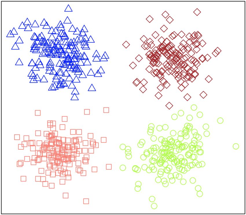
To monitor the performance, we implement our algorithm over four datasets
(Hepta, Tetra, TwoDiamonds, Lsun) with true labels which are publicly accessi-
ble from fundamental clustering problems suite (FCPS) [42] and one large-scale
dataset (LargeScale) randomly generated by ourselves. LargeScale dataset con-
sists of four clusters following Gaussian distributions with small variance and
distinct centers. Table 1 describes the properties of each dataset:
Table 1. Short descriptions of the datasets
Dataset Dimension # Data # Clusters Property
Hepta 3 212 7 Different densities
Tetra 3 400 4 Big and touching clusters
TwoDiamonds 2 800 2 Touching clusters
Lsun 2 400 3 Different shapes
LargeScale 4 262, 144 4 Numerous points
17Fig. 2. A visualization of LargeScale dataset
4.2 Parameter Selection
Our implementation is based on the approximate HE library HEAAN [1, 13].
We set HEAAN parameters (N, qL , h, χerr ) to satisfy 128-bit security, where N
is the ring dimension, qL is the initial modulus of a ciphertext, h is a hamming
weight of a secret polynomial, and χerr is the error distribution. As mentioned in
Section 2.2, we used Albrecht’s security estimator [2, 3] to estimate the bit secu-
rity of those HEAAN parameters. Note that since the modulus of the evaluation
2 2
key evk is qL , the input on the security estimator is a tuple (N, Q = qL , h, χerr ).
17
As a result, we set HEAAN parameters N = 2 and log qL = 1480, and followed
the default setting of HEAAN library [1] for error and secret distributions χerr ,
χenc andχkey .
We flexibly chose the clustering parameters T , Γ1 , Γ2 , ζ1 , ζ2 and t for each
dataset to optimize the implementation results. Let us denote the a tuple of pa-
rameters by params = (T, Γ1 , Γ2 , ζ1 , ζ2 , t). In the case of Hepta dataset, the best
choice of parameters was params = (5, 6, 6, 4, 4, 6), while params = (7, 6, 6, 5, 6, 6)
was the best for Tetra dataset, params = (8, 5, 5, 5, 6, 5) was the best for TwoDi-
amonds dataset, params = (5, 6, 5, 5, 8, 6) was the best for Lsun dataset, and
params = (5, 5, 5, 3, 3, 5) was the best for LargeScale dataset. We set the number
of dusts to be as small as possible (e.g., d = 8) to reduce the cost of bootstrap-
ping.
4.3 Experimental Results
In this subsection, we present experimental results on our mean-shift clustering
algorithm based on HEAAN. All experiments were performed on C++11 stan-
dard and implemented on Linux with Intel Xeon CPU E5-2620 v4 at 2.10GHz
processor.
In Table 2, we present the performance and quality of our algorithm on
various datasets. We use 8 threads for all experiments here. We describe the
18Table 2. Experimental results for various datasets with 8 threads
Quality Evaluation
Dataset Comp. Time Memory
Accuracy SilhCoeff
0.702
Hepta 25 min 10.7 GB 212/212
(0.702)
0.504
Tetra 36 min 10.7 GB 400/400
(0.504)
0.478
TwoDiamonds 38 min 9.6 GB 792/800
(0.485)
0.577
Lsun 24 min 9.4 GB -
(0.443)
0.781
LargeScale 82 min 20.7 GB 262127/262144
(0.781)
accuracy value by presenting both the number of well-classified points and the
total number of points. We present two silhouette coefficients; the one without
bracket is the silhouette coefficient of our clustering results, and the other one
with bracket is that of the true labels.
We complete the clustering on various datasets within a few dozens of min-
utes. In the case of FCPS datasets, their sizes are much smaller than the num-
ber of HEAAN plaintext slots we can manage. On the other hand, the size of
LargeScale dataset is big enough so that we can use full slots; therefore, we can
fully exploit SIMD of HEAAN for the LargeScale dataset. Consequently, the
performance of our algorithm for LargeScale dataset is quite nice in spite of its
huge size.
For all the five datasets, our algorithm achieves high accuracy. In the case
of Hepta, Tetra and LargeScale datasets, we succeed to label all data points by
its exact true label. For the TwoDiamonds dataset, we succeed to classify 792
points out of 800 points properly. Even for the rest 8 points, the label vector of
each point is close to its true label.
In the case of the Lsun dataset, our algorithm results in four clusters while
there are only three clusters in the true labels. Thereby, it is impossible to
measure the accuracy by comparing with the true labels, so one may think that
our algorithm is inadequate to the Lsun dataset. However, it is also reasonable to
classify the Lsun dataset with 4 clusters. In fact, our result shows even a better
quality in aspect of the silhouette coefficient. The silhouette coefficient for our
clustering result is 0.577, and that for the true labels is 0.443.
19We also checked the performance of our algorithm with several numbers of
threads for the Lsun dataset as described in Table 3. With a single thread, it
consumes 9.4 GB memory and takes 83 minutes. This result is much faster than
the result of the previous work in [29]; which takes 25.79 days to complete a
clustering process for the same dataset. Obviously we can speed up the perfor-
mance by using much more number of threads. For example, the running time
can be reduced to 16 minutes when using 20 threads with just small overhead
of memory.
Table 3. Experimental results for various # threads with the Lsun dataset
1 Thread 8 Threads 20 Threads
Time Memory Time Memory Time Memory
83 min 9.4 GB 24 min 9.4 GB 16 min 10.0 GB
Comparison to Freedman-Kisilev’s Method. The experimental results of
Freedman-Kisilev mean-shift clustering on the Tetra dataset under various p0 ,
the number of sampled points (see Section 2.4), shows how marginal p0 may
contaminate the performance. Note that our sampling method achieves 400/400
accuracy on the Tetra dataset with only 8 dusts.
In contrast, when p0 is either 8 or 16, Freedman-Kisilev algorithm even fails
to detect the correct modes from the original data. It detects only three clusters
while there actually exist four clusters; it classifies two different clusters as a sin-
gle cluster. Thus, the results on when p0 is either 8 or 16 are not even comparable
with the answer. This supports the argument that the KDE of Freedman-Kisilev
mean-shift may not fully represent the original KDE unless p0 is sufficiently big.
When p0 is bigger than 16, Freedman-Kisilev algorithm succeed to detect
four clusters as expected. However, the accuracy under each p0 = 32, 64, 128, 256
is 377/400, 368/400, 393/400, 399/400 respectively, while our sampling method
achieves 400/400 with only 8 dusts. This implies that the approximate KDE of
Freedman-Kisilev mean-shift may indicate modes with possible errors.
As a consequence, Freedman and Kisilev have to select substantially many
samples that can preserve the original KDE structure in some sense, while we
do not have such restriction on the number of dusts.
Acknowledgement
This work was supported in part by the Institute for Information & Commu-
nications Technology Promotion (IITP) Grant through the Korean Govern-
ment (MSIT), (Development of lattice-based post-quantum public-key cryp-
tographic schemes), under Grant 2017-0-00616, and in part by the National
20Research Foundation of Korea (NRF) Grant funded by the Korean Govern-
ment (MSIT) (No.2017R1A5A1015626). We also thank anonymous reviewers of
SAC’19 for very usual comments.
References
1. HEAAN Library. https://github.com/snucrypto/HEAAN, 2017.
2. M. R. Albrecht. A Sage Module for estimating the concrete security of Learning
with Errors instances., 2017. https://bitbucket.org/malb/lwe-estimator.
3. M. R. Albrecht, R. Player, and S. Scott. On the concrete hardness of learning with
errors. Journal of Mathematical Cryptology, 9(3):169–203, 2015.
4. N. Almutairi, F. Coenen, and K. Dures. K-means clustering using homomorphic
encryption and an updatable distance matrix: secure third party data clustering
with limited data owner interaction. In International Conference on Big Data
Analytics and Knowledge Discovery, pages 274–285. Springer, 2017.
5. C. Bonte and F. Vercauteren. Privacy-preserving logistic regression training. Cryp-
tology ePrint Archive, Report 2018/233, 2018. https://eprint.iacr.org/2018/
233.
6. F. Bourse, M. Minelli, M. Minihold, and P. Paillier. Fast homomorphic evaluation
of deep discretized neural networks. In Annual International Cryptology Confer-
ence, pages 483–512. Springer, 2018.
7. P. Bunn and R. Ostrovsky. Secure two-party k-means clustering. In Proceedings of
the 14th ACM Conference on Computer and Communications Security, CCS ’07,
pages 486–497, New York, NY, USA, 2007. ACM.
8. H. Chen, I. Chillotti, and Y. Song. Improved bootstrapping for approximate
homomorphic encryption. Cryptology ePrint Archive, Report 2018/1043, 2018.
https://eprint.iacr.org/2018/1043, To appear EUROCRYPT 2019.
9. H. Chen, R. Gilad-Bachrach, K. Han, Z. Huang, A. Jalali, K. Laine, and K. Lauter.
Logistic regression over encrypted data from fully homomorphic encryption. Cryp-
tology ePrint Archive, Report 2018/462, 2018. https://eprint.iacr.org/2018/
462.
10. J. H. Cheon, K. Han, and M. Hhan. Faster homomorphic discrete fourier transforms
and improved fhe bootstrapping. Cryptology ePrint Archive, Report 2018/1073,
2018. https://eprint.iacr.org/2018/1073, To appear IEEE Access.
11. J. H. Cheon, K. Han, S. M. Hong, H. J. Kim, J. Kim, S. Kim, H. Seo, H. Shim,
and Y. Song. Toward a secure drone system: Flying with real-time homomorphic
authenticated encryption. IEEE Access, 6:24325–24339, 2018.
12. J. H. Cheon, K. Han, A. Kim, M. Kim, and Y. Song. Bootstrapping for approximate
homomorphic encryption. In Annual International Conference on the Theory and
Applications of Cryptographic Techniques, pages 360–384. Springer, 2018.
13. J. H. Cheon, A. Kim, M. Kim, and Y. Song. Homomorphic encryption for arith-
metic of approximate numbers. In International Conference on the Theory and
Application of Cryptology and Information Security, pages 409–437. Springer, 2017.
14. J. H. Cheon, D. Kim, D. Kim, H. H. Lee, and K. Lee. Numerical methods for
comparison on homomorphically encrypted numbers. Cryptology ePrint Archive,
Report 2019/417, 2019. https://eprint.iacr.org/2019/417.
15. J. H. Cheon, D. Kim, Y. Kim, and Y. Song. Ensemble method for privacy-
preserving logistic regression based on homomorphic encryption. IEEE Access,
2018.
2116. I. Chillotti, N. Gama, M. Georgieva, and M. Izabachene. Faster fully homomorphic
encryption: Bootstrapping in less than 0.1 seconds. In International Conference on
the Theory and Application of Cryptology and Information Security, pages 3–33.
Springer, 2016.
17. I. Chillotti, N. Gama, M. Georgieva, and M. Izabachène. Faster packed homo-
morphic operations and efficient circuit bootstrapping for tfhe. In International
Conference on the Theory and Application of Cryptology and Information Security,
pages 377–408. Springer, 2017.
18. H. Cho, D. J. Wu, and B. Berger. Secure genome-wide association analysis using
multiparty computation. Nature biotechnology, 36(6):547, 2018.
19. J. L. Crawford, C. Gentry, S. Halevi, D. Platt, and V. Shoup. Doing real work
with fhe: The case of logistic regression. 2018.
20. I. S. Dhillon, E. M. Marcotte, and U. Roshan. Diametrical clustering for identifying
anti-correlated gene clusters. Bioinformatics, 19(13):1612–1619, 2003.
21. M. C. Doganay, T. B. Pedersen, Y. Saygin, E. Savaş, and A. Levi. Distributed
privacy preserving k-means clustering with additive secret sharing. In Proceedings
of the 2008 International Workshop on Privacy and Anonymity in Information
Society, PAIS ’08, pages 3–11, New York, NY, USA, 2008. ACM.
22. R. O. Duda, P. E. Hart, and D. G. Stork. Pattern classification. John Wiley &
Sons, 2012.
23. D. Freedman and P. Kisilev. Fast mean shift by compact density representation.
In 2009 IEEE Conference on Computer Vision and Pattern Recognition, pages
1818–1825. IEEE, 2009.
24. C. Gentry. A fully homomorphic encryption scheme. PhD thesis, Stanford Univer-
sity, 2009. http://crypto.stanford.edu/craig.
25. R. Gilad-Bachrach, N. Dowlin, K. Laine, K. Lauter, M. Naehrig, and J. Wernsing.
Cryptonets: Applying neural networks to encrypted data with high throughput
and accuracy. In International Conference on Machine Learning, pages 201–210,
2016.
26. R. E. Goldschmidt. Applications of division by convergence. PhD thesis, Mas-
sachusetts Institute of Technology, 1964.
27. K. Han, S. Hong, J. H. Cheon, and D. Park. Logistic regression on homomorphic
encrypted data at scale. 2019.
28. G. Jagannathan and R. N. Wright. Privacy-preserving distributed k-means cluster-
ing over arbitrarily partitioned data. In Proceedings of the Eleventh ACM SIGKDD
International Conference on Knowledge Discovery in Data Mining, KDD ’05, pages
593–599, New York, NY, USA, 2005. ACM.
29. A. Jäschke and F. Armknecht. Unsupervised machine learning on encrypted data.
In International Conference on Selected Areas in Cryptography, pages 453–478.
Springer, 2018.
30. A. Kim, Y. Song, M. Kim, K. Lee, and J. H. Cheon. Logistic regression model train-
ing based on the approximate homomorphic encryption. BMC Medical Genomics,
11(4):83, Oct 2018.
31. M. Kim, Y. Song, S. Wang, Y. Xia, and X. Jiang. Secure logistic regression based
on homomorphic encryption: Design and evaluation. JMIR Med Inform, 6(2):e19,
Apr 2018.
32. D. Liu. Practical fully homomorphic encryption without noise reduction. Cryptol-
ogy ePrint Archive, Report 2015/468, 2015. https://eprint.iacr.org/2015/468.
33. X. Liu, Z. L. Jiang, S.-M. Yiu, X. Wang, C. Tan, Y. Li, Z. Liu, Y. Jin, and J. Fang.
Outsourcing two-party privacy preserving k-means clustering protocol in wireless
22sensor networks. In 2015 11th International Conference on Mobile Ad-hoc and
Sensor Networks (MSN), pages 124–133. IEEE, 2015.
34. M. B. Malik, M. A. Ghazi, and R. Ali. Privacy preserving data mining techniques:
current scenario and future prospects. In Computer and Communication Technol-
ogy (ICCCT), 2012 Third International Conference on, pages 26–32. IEEE, 2012.
35. F. Meskine and S. Nait-Bahloul. Privacy preserving k-means clustering: A survey
research. 9, 03 2012.
36. F. Pouget, M. Dacier, et al. Honeypot-based forensics. In AusCERT Asia Pacific
Information Technology Security Conference, 2004.
37. P. J. Rousseeuw. Silhouettes: a graphical aid to the interpretation and validation
of cluster analysis. Journal of computational and applied mathematics, 20:53–65,
1987.
38. J. Sakuma and S. Kobayashi. Large-scale k-means clustering with user-centric pri-
vacy preservation. In Proceedings of the 12th Pacific-Asia Conference on Advances
in Knowledge Discovery and Data Mining, PAKDD’08, pages 320–332, Berlin, Hei-
delberg, 2008. Springer-Verlag.
39. S. Samet, A. Miri, and L. Orozco-Barbosa. Privacy preserving k-means clustering
in multi-party environment., 01 2007.
40. C. Su, F. Bao, J. Zhou, T. Takagi, and K. Sakurai. Privacy-preserving two-party
k-means clustering via secure approximation. In Proceedings of the 21st Inter-
national Conference on Advanced Information Networking and Applications Work-
shops - Volume 01, AINAW ’07, pages 385–391, Washington, DC, USA, 2007. IEEE
Computer Society.
41. C. A. Sugar and G. M. James. Finding the number of clusters in a dataset: An
information-theoretic approach. Journal of the American Statistical Association,
98(463):750–763, 2003.
42. A. Ultsch. Clustering with som: U* c. In Proc. Workshop on Self-Organizing Maps,
pages 75–82, Paris, France, 2005. Datasets available at https://www.uni-marburg.
de/fb12/arbeitsgruppen/datenbionik/data?language_sync=1.
43. J. Vaidya and C. Clifton. Privacy-preserving k-means clustering over vertically
partitioned data. In Proceedings of the Ninth ACM SIGKDD International Con-
ference on Knowledge Discovery and Data Mining, KDD ’03, pages 206–215, New
York, NY, USA, 2003. ACM.
44. K. J. Vinoth and V. Santhi. A brief survey on privacy preserving techniques in
data mining. IOSR Journal of Computer Engineering (IOSR-JCE), pages 47–51,
2016.
45. S. Wang, Y. Zhang, W. Dai, K. Lauter, M. Kim, Y. Tang, H. Xiong, and X. Jiang.
Healer: Homomorphic computation of exact logistic regression for secure rare dis-
ease variants analysis in gwas. Bioinformatics, 32(2):211–218, 2016.
46. Y. Wang. Notes on two fully homomorphic encryption schemes without bootstrap-
ping. IACR Cryptology ePrint Archive, 2015:519, 2015.
23You can also read