Towards an Intelligent Edge: Wireless Communication Meets Machine Learning - arXiv

Page created by Edwin Robbins
 
CONTINUE READING
Towards an Intelligent Edge: Wireless Communication Meets Machine Learning - arXiv
Towards an Intelligent Edge:
        Wireless Communication Meets Machine Learning
        Guangxu Zhu1, Dongzhu Liu1, Yuqing Du1, Changsheng You1, Jun Zhang2 and Kaibin Huang1

Abstract
The recent revival of artificial intelligence (AI) is revolutionizing almost every branch of science and technology. Given
the ubiquitous smart mobile gadgets and Internet of Things (IoT) devices, it is expected that a majority of intelligent
applications will be deployed at the edge of wireless networks. This trend has generated strong interests in realizing an
“intelligent edge” to support AI-enabled applications at various edge devices. Accordingly, a new research area, called
edge learning, emerges, which crosses and revolutionizes two disciplines: wireless communication and machine
learning. A major theme in edge learning is to overcome the limited computing power, as well as limited data, at each
edge device. This is accomplished by leveraging the mobile edge computing (MEC) platform and exploiting the
massive data distributed over a large number of edge devices. In such systems, learning from distributed data and
communicating between the edge server and devices are two critical and coupled aspects, and their fusion poses many
new research challenges. This article advocates a new set of design principles for wireless communication in edge
learning, collectively called learning-driven communication. Illustrative examples are provided to demonstrate the
effectiveness of these design principles, and unique research opportunities are identified.

I.    Introduction
We are witnessing a phenomenal growth in global data traffic, accelerated by the increasing popularity of
mobile devices, e.g., smartphones, tablets and sensors. According to the intersectional data corporation
(IDC), there will be 80 billion devices connected to the Internet by 2025, and the global data will reach 163
zettabytes, which is ten times of the data generated in 2016 [1]. The unprecedented amount of data, together
with the recent breakthroughs in artificial intelligence (AI), inspire people to envision ubiquitous computing
and ambient intelligence, which will not only improve our life qualities but also provide a platform for
scientific discoveries and engineering innovations. In particular, this vision is driving the industry and
academia to vehemently invest in technologies for creating an intelligent (network) edge, which supports
emerging application scenarios such as smart city, eHealth, eBanking, intelligent transportation, etc. This has
led to the emergence of a new research area, called edge learning, which refers to the deployment of
machine-learning algorithms at the network edge [2]. The key motivation of pushing learning towards the
edge is to allow rapid access to the enormous real-time data generated by the edge devices for fast AI-model
training, which in turn endows on the devices human-like intelligence to respond to real-time events.
Traditionally, training an AI model, especially a deep model, is computation-intensive and thus can only be
supported at powerful cloud servers. Riding the recent trend in developing the mobile edge computing
(MEC) platform, training an AI model is no longer exclusive for cloud servers but also affordable at edge
servers. Particularly, the network virtualization architecture recently standardized by 3GPP is able to support
edge learning on top of edge computing [3]. Moreover, the latest mobile devices are also armed with high-
performance central-processing units (CPUs) or graphics processing units (GPUs) (e.g., A11 bionic chip in
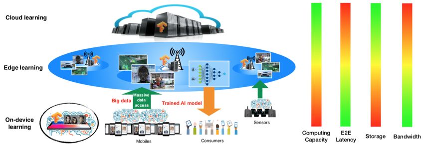
iPhone X), making them capable in training some small-scale AI models. The coexistence of cloud, edge and
on-device learning paradigms has led to a layered architecture for in-network machine learning, as shown in
Fig. 1. Different layers possess different data processing and storage capabilities, and cater for different types
of learning applications with distinct latency and bandwidth requirements.

G. Zhu, D. Liu, Y, Du, C, You and K. Huang are with the Dept. of Electrical and Electronic Engineering at the University of
Hong Kong, Hong Kong. Email: {gxzhu,dzliu,yqdu,csyou,huangkb}@eee.hku.hk. Corresponding Author: K. Huang.

J. Zhang is with the Dept. of Electronic and Computer Engineering at the Hong Kong University of Science and Technology,
Hong Kong. Email: eejzhang@ust.hk
                                                               !1
Towards an Intelligent Edge: Wireless Communication Meets Machine Learning - arXiv
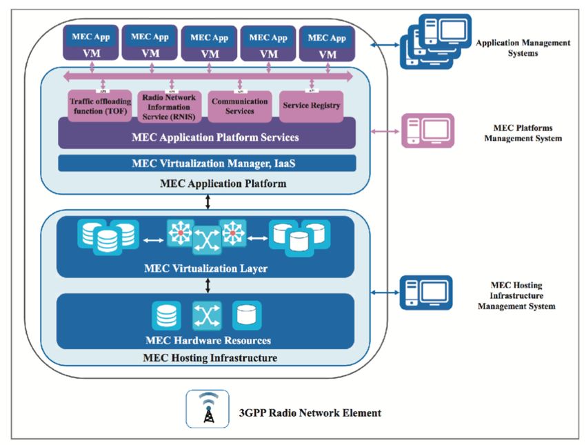
Compared with cloud and on-device learning, edge learning has its unique strengths. First, it has the most
balanced resource support (see Fig. 1), which helps achieving the best tradeoff between the AI-model
complexity and the model-training speed. Second, given its proximity to data sources, edge learning
overcomes the drawback of cloud learning that fails to process real-time data due to excessive propagation
delay and also network congestion caused by uploading data to the cloud. Furthermore, the proximity gives
an additional advantage of location-and-context awareness. Last, compared with on-device learning, edge
learning achieves much higher learning accuracy by supporting more complex models and more importantly
aggregating distributed data from many devices. Due to the all-rounded capabilities, edge learning can
support a wide spectrum of AI models to power a broad range of mission-critical applications, such as auto-
driving, rescue-operation robots, disaster avoidance and fast industrial control. Nevertheless, edge learning is
at its nascent stage and thus remains a largely uncharted area with many open challenges.

Fig. 1. Layered in-network machine learning architecture.
The main design objective in edge learning is the fast intelligence acquisition from the rich but highly
distributed data at subscribed edge devices. This critically depends on data processing at edge servers, as
well as efficient communication between edge servers and edge devices. Compared with increasingly high
processing speeds at edge servers, communication suffers from hostility of wireless channels (e.g., pathloss,
shadowing, and fading), and consequently forms the bottleneck for ultra-fast edge learning. In order to distill
the shared intelligence from distributed data, excessive communication latency may arise from the need of
uploading to an edge server a vast amount of data generated by millions to billions of edge devices, as
illustrated in Fig. 1. As a concrete example, the Tesla's AI model for auto-driving is continuously improved
using RADAR and LIDAR sensing data uploaded by millions of Tesla vehicles on the road, which can
amount to about 4,000 GB for one car per day. Given the enormity in data and the scarcity of radio
resources, how to fully exploit the distributed data in AI-model training without incurring excessive
communication latency poses a grand challenge for wireless data acquisition in edge learning.
Unfortunately, the state-of-the-art wireless technologies are incapable of tackling the challenge. The
fundamental reason is that the traditional design objectives of wireless communications, namely
communication reliability and data-rate maximization, do not directly match that of edge learning. This
means that we have to break away from the conventional philosophy in traditional wireless communication,
which can be regarded as a “communication-computing separation” approach. Instead, we should exploit the
coupling between communication and learning in edge learning systems. To materialise the new philosophy,
we propose in this article a set of new design principles for wireless communication in edge learning,
collectively called learning-driven communication. In the following sections, we shall discuss specific
research directions and provide concrete examples to illustrate this paradigm shift, which cover key
communication aspects including multiple access, resource allocation and signal encoding, as summarized
in Table 1. All of these new design principles share a common principle as highlighted below.

                                                            !2
Towards an Intelligent Edge: Wireless Communication Meets Machine Learning - arXiv
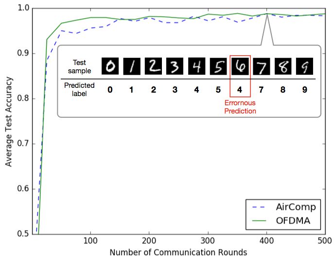
Principle of Learning-Driven Communication - Fast Intelligence Acquisition
   Efficiently transmit data or learning-relevant information to speed up and improve AI-model training at
                                                  edge servers.

         Table 1. Conventional Communication versus Learning-Driven Communication

   Commun. Tech.           Item           Conventional Commun.                 Learning-Driven Commun.

                           Target     Decoupling messages from users        Computing func. of distributed data
   Multiple access
     (Section II)        Case study                OFDMA                    Model-update averaging by AirComp

Resource Allocation   Target            Maximize sum-rate or reliability         Fast intelligence acquisition
   (Section III)    Case study          Reliability-based retransmission      Importance-aware retransmission

                                       Optimal tradeoffs between rate and       Latency minimization while
                           Target
  Signal Encoding                            distortion/reliability           preserving the learning accuracy
    (Section IV)                       Quantization, adaptive modulation
                         Case study                                             Grassmann analog encoding
                                                and polar code

At the high level, learning-driven communication integrates wireless communication and machine leaning
that have been rapidly advancing as two separate disciplines with few cross-paths. In this paper, we aim at
providing a roadmap for this emerging and exciting area by highlighting research opportunities, shedding
light on potential solutions, as well as discussing implementation issues.

II. Learning-Driven Multiple Access
a) Motivation and Principle
In edge learning, the involved training data (e.g., photos, social-networking records, and user-behaviour data)
are often privacy sensitive and large in quantity. Thus uploading them from devices to an edge server for
centralized model training may not only raise a privacy concern but also incur prohibitive cost in
communication. This motivates an innovative edge-learning framework, called federated learning, which
features distributed learning at edge devices and model-update aggregation at an edge server [4]. Federated
learning can effectively address the aforementioned issues as only the locally computed model updates,
instead of raw data, are uploaded to the server. A typical federated-learning algorithm alternates between two
phases, as shown in Fig. 2 (a). One is to aggregate distributed model updates over a multi-access channel and
apply their average to update the AI-model at the edge server. The other is to broadcast the model under
training to allow edge devices to continuously refine their individual versions of the model. This learning
framework is used as a particular scenario of edge learning in this section to illustrate the new design
principle of learning-driven multiple access.
Model-update uploading in federated learning is bandwidth-consuming as an AI model usually comprises
millions to billions of parameters. Overall the model updates by thousands of edge devices may easily
congest the air-interface, making it a bottleneck for agile edge learning. The said bottleneck is arguably an
artifact of the classic approach of communication-computing separation. Existing multiple access
technologies such as orthogonal frequency-division multiple access (OFDMA) and code division multiple
access (CDMA) are purely for rate-driven communication and fail to adapt to the actual learning task. The
need for enabling fast edge learning from massive distributed data calls for a new design principle for
multiple access. In this section, we present learning-driven multiple access as the solution, and showcase a
particular technique under this new principle.

                                                       !3
Towards an Intelligent Edge: Wireless Communication Meets Machine Learning - arXiv
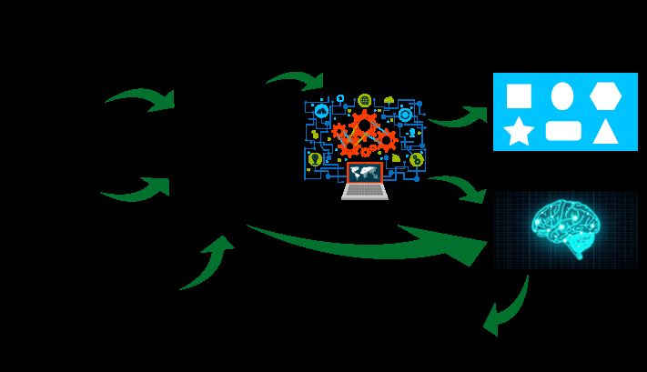
The key innovation underpinning the learning-driven multiple access is to exploit the insight that the
learning task involves computing some aggregating function (e.g., averaging or finding the maximum) of
multiple data samples, rather than decoding individual samples as in the existing scheme. For example, in
federated learning, the edge server requires the average of model updates rather than their individual values.
On the other hand, the multi-access wireless channel by itself is a natural data aggregator: the simultaneously
transmitted analog-waves by different devices are automatically superposed at the receiver but weighed by
the channel coefficients. The above insights motivate the following design principle for multiple access in
edge learning. It changes the traditional philosophy of “overcoming interference” to the new one of
“harnessing interference”.

                                 Principle of Learning-Driven Multiple Access
  Unique characteristics of wireless channels, such as broadcast and superposition, should be exploited for
                 functional computation over distributed data to accelerate edge learning.

                                                                                                                                                              + SB-otmef
                                                                                                                                                        nocaeb rewop
                                                                                                                                                 Local Model
                                                                                                                                                   Update
                                                                                                                             TI+TP
                                                                                                                                                                      Local
                                                                                                                )gnorts(                                      + SBDataset
                                                                                                                                                                  -otmef
                                                         Distributed                                                                                         nocaeb rewop
             Global Model   M                           Model Updates
                                                                                                                      )kaeTwI+( TP
                                                                                                                                                        TI
                                                                                                                )gnortsLocal
                                                                                                                       (     Model M1                     + SB-otmef
                                                                                                                                                         nocaeb rewop
                                                                                                                      )kaeTwI+( TP
                                                                                                                                   ..            Local Model
                                                                                                                                                                                 SB
                                                                                                                                    .              Update
                                                                                                                                                        TI
                                         Edge Server                                                                                                               Local
                                                                                                                )gnorts(                                          Dataset
         Global Model
            Update                                      Broadcast Model                                              )kaew(                                                      SB
                                   Update Aggregation
                                      1 X
                                                             d n a n o i t a m r o f n I f oTIg n i l p u o c e D g o l a
                                                         Under Training
                                   M=     Mk                                  Local Model M
                                      K
                                              k                                                      s r e f s n a rT r e w                  K

                                                                                                                  SB
                                                             d(a)n a n o i t a m r o f n I f o g n i l p u o c e D g o l a
                                                                                                     s r e f s n a rT r e w
                                                                                                      10
                                                                                                           7

                                                                                                                                                         AirComp

                                                             dna noitam rofnI fo gnilpuoceD gola      10 6
                                                                                                                                                         OFDMA with K=50
                                                                                                                                                         OFDMA with K=100
                                                                                                                                                         OFDMA with K=500
                                                               Communication Latency (OFDM Symbols)

                                                                                                     s r e f s n a rT r e w
                                                                                                      10 5

                                                                                                      10 4

                                                                                                                                                        32
                                                                                                      10 3

                                                                                                      10 2
                                                                                                                                                        32

                                                                                                      10 1
                                                                                                          10   15   20        25        30       35      40      45         50
                                                                                                                           Transmit SNR per User (dB)

                                                                                                                                                        32
                                                              (b)

Fig. 2. (a) Federated learning using wirelessly distributed data. (b) Performance comparison between AirComp and
OFDMA in test accuracy (left) and communication latency (right). The implementation details are specified as follows.
For AirComp, model parameters are analog-modulated and each sub-band is dedicated for single-parameter transmis-
sion; truncated-channel inversion (power control) under the transmit-power constraint is used to tackle the channel fad-
ing. For OFDMA, model parameters are first quantized into a bit sequence (16-bit per parameter). Then adaptive
MQAM modulation is adopted to adapt the data rate to the channel condition such that the spectrum efficiency is max-
imized while the target bit-error-rate of 10-3 is maintained.

                                                              !4
Following the new principle, the superposition nature of the multi-access channel suggests that by using
linear-analog modulation and pre-channel-compensation at the transmitter, the “interference” caused by
concurrent data transmission can be exploited for fast data aggregation. This intuition has been captured by a
recently proposed technique called over-the-air computation (AirComp) [5], [6]. By allowing simultaneous
transmission, AirComp can dramatically reduce the multiple access latency by a factor equal to the number
of users (i.e., 100 times for 100 users). It provides a promising solution for overcoming the communication
latency bottleneck in edge learning.

b) Case Study: Over-the-Air Computation for Federated Learning
Experiment settings: Consider a federated learning system with one edge server and K=100 edge devices.
For exposition, we consider the learning task of handwritten-digit recognition using the well-known MNIST
dataset that consists of 10 categories ranging from digit “0” to “9” and a total of 60000 labeled training data
samples. To simulate the distributed mobile data, we randomly partition the training samples into 100 equal
shares, each of which is assigned to one particular device. The classifier model is implemented using a 4-
layer convolutional neural network (CNN) with two 5x5 convolution layers, a fully connected layer with 512
units and ReLu activation, and a final softmax output layer (582,026 parameters in total).
AirComp versus OFDMA: During the federated model training, in each communication round, local
models trained at edge devices (using e.g., stochastic gradient descend) are transmitted and aggregated at the
edge server over a shared broadband channel that consists of Ns=1000 orthogonal sub-channels. Two
multiple access schemes, namely the conventional OFDMA and the proposed AirComp, are compared. They
mainly differ in how the available sub-channels are shared. For OFDMA, the 1000 sub-channels are evenly
allocated to the K edge devices, so each device uploads its local model using only fractional bandwidth that
reduces as K grows. Model averaging is performed by the edge server after all local models are reliably
received, and thus the communication latency is determined by the slowest device. In contrast, the AirComp
scheme allows every device to use the full bandwidth so as to exploit the “interference” for direct model
averaging over the air. The latency of AirComp is thus independent of the number of accessing devices.
Performance: The learning accuracy and communication latency of the two schemes are compared in Fig. 2
(b) under the same transmit signal-to-noise ratio (SNR) per user. As shown at the left-hand side of Fig. 2 (b),
although AirComp is expected to be more vulnerable to channel noise, it is interesting to see that the two
schemes are comparable in learning accuracy. Such accurate learning of AirComp is partly due to the high
expressiveness of the deep neural network which makes the learnt model robust against perturbation by
channel noise. The result has a profound and refreshing implication that reliable communication may not be
the primary concern in edge learning. Essentially, AirComp exploits this relaxation on communication
reliability to trade for a low communication latency as shown at the right-hand side of Fig. 2 (b). The latency
gap between the two schemes is remarkable. Without compromising the learning accuracy, AirComp can
achieve a significant latency reduction ranging from 10x to 1000x. In general, the superiority in latency of
AirComp over OFDMA is more pronounced in the low SNR regime and dense-network scenarios.

c) Research Opportunities
The new design principle of learning-driven multiple access points to numerous research opportunities, some
of which are described as follows.
•   Robust learning with imperfect AirComp. Wireless data aggregation via AirComp requires channel
    pre-equalization at the transmitting devices. Inaccurate channel estimation and non-ideal hardware at the
    low-cost edge devices may cause imperfect equalization and thus distort the aggregated data. For
    practical implementation, it is important to characterize the effects of the imperfect AirComp on the
    performance of edge learning, based on which new techniques can be designed to improve the learning
    robustness.
•   Asynchronous AirComp. Successful implementation of AirComp requires strict synchronization
    between all the participating edge devices. This may be hard to achieve when the devices exhibit high
                                                      !5
mobility or the learning system is highly dynamic with the participating devices changing frequently
    over time. To enable ultra-fast data aggregation in these scenarios, new schemes operated in an
    asynchronous manner or with a relaxed requirement on synchronization are desirable.
•   Generalization to other edge-learning architectures. The proposed AirComp solution targets
    federated-learning architecture. It may not be applicable for other architectures where the edge server
    needs to perform more sophisticated computation over the received data than simple averaging. How to
    exploit the superposition property of a multi-access channel to compute more complex functions is the
    main challenge in generalizing the current learning-driven multiple access design to other architectures.

III. Learning-Driven Radio Resource Management
a) Motivation and Principle
Based on the traditional approach of communication-computing separation, existing methods of radio-
resource management (RRM) are designed to maximize the efficiency of spectrum utilization by carefully
allocating the scarce radio resources such as power, frequency band and access time. However, such an
approach is no longer effective in edge learning, as it fails to exploit the subsequent learning process for
further performance improvement. This motivates us to propose the following design principle for RRM in
edge learning.

                                    Principle of Learning-Driven RRM
    Radio resources should be allocated based on the value of transmitted data so as to optimize the edge-
                                           learning performance.

Conventional RRM assumes that the transmitted messages have the same value for the receiver. The
assumption makes sum-rate maximization a key design criterion. When it comes to edge learning, the rate-
driven approach is no longer efficient as some messages tend to be more valuable than others for training an
AI model.
In this part, we introduce a representative technique following the above learning-driven design principle,
called importance-aware resource allocation, which takes the data importance into account in resource
allocation. The basic idea of this new technique shares some similarity with a key area in machine learning
called active learning. Principally, active learning is to select important samples from a large unlabelled
dataset for labelling (by querying an oracle) so as to accelerate model training with a labelling budget [7]. A
widely adopted measure of (data) importance is uncertainty. To be specific, a data sample is more uncertain
if it is less confidently predicted by the current model. For example, a cat photo that is classified as “cat”
with a correctness probability of 0.6 is more uncertain than that of a probability of 0.8. A commonly used
uncertainty measure is entropy, a notion from information theory. As its evaluation is complex, a heuristic
but simple alternative is the distance of a data sample from the decision boundaries of the current model.
Taking support vector machine (SVM) as an example, a training data sample near to the decision boundary is
likely to become a support vector, thereby contributing to defining the classifier. In contrast, a sample away
from boundaries makes no such contribution.
Compared with active learning, learning-driven RRM has its additional challenges given the volatile wireless
channels. In particular, besides data importance, it needs to consider radio-resource allocation to ensure a
certain level of reliability in transmitting a data sample. A basic diagram of learning-driven RRM is
illustrated in Fig.3 (a). In the following, we will provide a concrete case-study for illustration.

b) Case Study: Importance-Aware Retransmission for Wireless Data Acquisition
Experiment settings: Consider an edge learning system where a classifier is trained at the edge server based
on SVM, with data collected from distributed edge devices. The acquisition of high-dimensional training-
data samples is bandwidth consuming and relies on a noisy data channel. On the other hand, a low-rate
reliable channel is allocated for accurately transmitting small-size labels. The mismatch between the labels
                                                      !6
and noisy data samples at the edge server may lead to an incorrectly learnt model. To tackle the issue,
importance-aware retransmission with coherent combining is used to enhance the data quality. The radio
resource is specified by the limited transmission budgets with N=4000 samples (new/retransmitted). To train
the classifier, we use the MNIST dataset described in Section II-b) and choose the relatively less
differentiable class pair of ‘3' and ‘5' to focus on a binary classification case.
                                                        0.91
                                                        0.89                                                                                                                                                                                      0.91
                                                                                   Channel State Information                                                                           Radio                                                                                                                                                          0.9
                                                        0.87                            h1, h2, h3…
                                                                                                                                                                                     Resource
                                                                                                                                                                                                                       Learning                   0.89       Trained Model
                                                                                                                                                                                                                        Model                                                                                                                         0.8
                                                                                                                                                                                     Allocation
                                                                                      Received Data Samples                                                                                                                                       0.87
                                                        0.85                              S1, S2, S3…
                                                                               0.91                                                                                                                                                                       Learning Model
                                                                                                                                                                                                                                                  E.g. Classification using SVM                where y(i) is given0.8in (
                                                                                                                                                                                           Importance
                                                        0.83                                                                                                                                 Level
                                                                                                                                                                                                                                                  0.85
                                                                                                                                                                                                                                       Support Vector          Margin:     = min |wT xk + b|
                                                                                                                                                                                                                                                                                 k
                                                                                                                                                                                                                                                                                               the combined signal for
                                                                               0.89                                                                                                                                                                                                            machine learning are0.8rea
                                             Accuracy

                                                                                                                                                                                                                                                                       +         +

                                                        0.81                                                                                                                                                                                      0.83             +
                                                                                                                                                                                                                                                                           +
                                                                                                                                                                                                                                                                                 +             clips or video clips). As
                                                                                                                                                                                                                                                                             +
                                                                               0.87                                                                                       Importance            Real-time Model                                                                                x̂(T ) is given as 0.8

                                                                                                                                                                                                                                       Accuracy
                                                                                                                                                                                                                                                                         +           +
                                                                                                                                                                           Evaluation                                                             0.81                 +

                                                                                                                                                                                                                                                                                                                                           Accuracy
                                                       0.79
                                                      0.9                      0.85                                                                                                                                                           0.91 Hyperplane: wT x + b = 0
                                                                                                                                                                                                                                                                           +

                                                                                                                                                                                                                                                                                                                                                0.8
                                                                                                                                                                                                                                                                                                                                              SNR(T
                                                       0.77Server              0.83                                                                                                                                                               0.79
         Edge Devices                                Edge
                                                     0.88                                                                                                                                                                                     0.89                                                                                                    0.7
                                                                    Accuracy

                                                                                                                                                                                                  where the coefficient 2
        Edge Devices                                    0.75                   0.81                                                                                                                     Low-rate noiseless label channel        0.77
                                                                                                                                                                                                                                              0.87
                                                                                                                                                                                                  fact that only the noise
                                                                                                                                                                                                        High-rate noisy data channel
                                                     0.86                                                                                                                                            2                      0.7               TDMA

                                                                                                                                                                                                    2 affects the received
                                                       0.9
                                         0.79                                 Importance Aware        Edge Devices
                                                                                                            Retransmission                      0.75            Edge Server
                            0.73                                    (a)                                          Communication System Model  0.85                                                 MRC and its value grow
                          0.84           0.77        0.88                     Channel Aware            Retransmission
                                                                                                    Without        Retransmission
                                                                                                                             Figure 1. Edge learning system.                                      increases. The SNR        0.7
                                                                                                                                                                                                                             exp
                                                                                                                                                0.73
                                                                                                                                             0.83                                                                         Impo
                            0.71                                              Without Retransmission                                                                                              of a received data samp
                                                                                                    device    for   acquiring     a  new      sample      or   requesting        the   previ-                             Chan
                                                                                                                                                                                                                            0.7

                                                                                                                                                                                                                                   Accuracy
                          0.82           0.75        0.86                                                                                                                                         the   retransmission     decis
                                                               0.91                                 ously scheduled device for retransmission   0.71
                                                                                                                                             0.81                  to improve sample                                      With
                            0.69                                                           Importance        Aware     Retransmission                                                                  Transmission Budge
                                          Accuracy

                                  0      0.731000
                                                0.9 0.84             2000                  3000quality.         Retransmission
                                                                                                                       4000 is controlled by stop-and-wait ARQ. resource or a latency                                       0.7
                                              0.9                                          Channel       Aware     Retransmission
                           0.8                                 0.89                                 The positiveWithout      Retransmission
                                                                                                                     acknowledgment          0.79
                                                                                                                                                0.69 or negative ACK (NACK) transmission
                                                                                                                                               (ACK)                                                           40 budget for
                                         0.71      Transmission Budget NWithout                        Retransmission
                                                                                                    is sent to the target device based on                0 whether the currently    1000 to be N 2000          symbol blocks0.6
                          0.78
                                              0.88 0.82
                                             0.88              0.87           0.91                  received sample at the server
                                                                                                                                               0.91
                                                                                                                                             0.77 satisfies a pre-defined quality duration
                                                    0.9
                                                                                               0.9 requirement as elaborated in the sequel. Each edge device Transmission
                                                                                                                                                                                                            40(in  symbol
                                                                                                                                                                                                                       Budg  blo

                                                                                                                                                                                                                                                                                                       Average Number of Retransmissions
                                         0.69                                                                                                                                                                  35
                                                                                                     Accuracy

                                                        0.9           0.9                                                                                                                    is
                                              0        0.80.9 1000                 2000
                                                                                     0.9                 3000                   4000 0.75      0.89
                                              0.86             0.850.88       0.89                  assumed
                                                                                                clean            to have backlogged data. Upon receiving a request
                          0.76               0.86 0.88               Transmission Budget               Nsamples                                                                                          40

                                                                                                                                                                                                                                                                                                  Average Number of Retransmissions
                                                                                              0.88
                                                      0.88                            Quality       from the server, a device either transmits a randomly picked                                            3530Importance
                                                     0.780.88                 0.870.88                                                       0.73
                                                                                                                                               0.87
                                                                                                    new sample from its buffer or retransmits the previous sample.
                          0.74                0.840.86
                                             0.84              0.830.86                       0.86                                                                                                                Channel A
                                                                                                       The    noisy   data   channel    between       is  assumed       to  follow    block-             35
                                                                                                                                                                                                  where K denotes         the Re
                                                                                                                                                                                                                               nu
                                                                                                                                                          Test Accuracy

                                                      0.86                                                                                                                                                        Without
                                                                                                                                             0.71
                                                                                                                           Accuracy

                                                     0.760.86                 0.850.86              fading    where
                                                                                                         Channel
                                                                                                                                 clean samples
                                                                                                                        the channel
                                                                                                                    Aware                      0.85 remains static within a of retransmissions
                                                                                                                                          coefficient                                                       3025           spent
                          0.72                0.820.840.84 0.810.84
                                             0.82                                             0.84
                                                                                                    symbol     block Aware
                                                                                                         Uncertainty     and is independent            and    identically        distributed             30
                                                                              0.830.84                                                       0.69
                                                     0.740.84
                                                                                                    (i.i.d.)  over different blocks. 0.83
                                                                                                         Confidence Level
                                                                                                                                                During0 the i-th symbol        1000block, B. Learning   2000        Model 3
                                                                               Accuracy
                                                                               Accuracy

                                                                                                                                                       Accuracy

                                                               0.79  0.82                     0.82       Without Retransmission (i)                                                                         2520
                                                                                                                                                                                                                                    Accuracy
                           0.7                0.8 0.82
                                                0.8 0.82                      0.81                  the  device    sends    the  data   x
                                                                                                                                  Quality       using
                                                                                                                                          Channel        linear analog modulation,
                                                                                                                                                     Aware                                             For
                                                                                                                                                                                                         25 the task of edge
                                                                                                                                               0.81byAware                            Transmission              Budget       N
                                                                                                                                      Accuracy

                                                                                                                                                                                     Accuracy

                                                     0.720.82                       0.82            yielding the received signalUncertainty given                                                 of a classifier model b
                                                                                          Accuracy

                                                                      0.8                      0.8
                                                                                                        Accuracy

                                                               0.77                                                                    sConfidence Level
                                                                                                                Accuracy

                                                                                                                                                                          Accuracy

                                               10000.8 0.80.8 1500            0.79 0.8 2500                                                                                                       machine20 20
                                                                                                                                                                                                               (SVM). Prior
                                                                                                                                                                                                               15
                                                                                                                                                  Average

                                                                                                                                          Without
                               0     500     0.78
                                              0.78     0.7
                                                                            2000                         3000             3500              4000 P Retransmission
                                                                                                                                               0.79
                                                                     0.78Time Slot            0.78                      y(i) = h(i)                     x(i) + z(i) ,                      (1) sever has a small set o
                                                               0.75           0.77                                                          E[kxk2 ]                                              L0 . This allows the con
                                                  0.780.78                                                                                     0.77
                                             0.76
                                              0.76
                                                         0.78
                                                           0          500       10000.78     1500
                                                                                              0.76 where2000               2500 cleanclean  samples
                                                                                                                                          3000         clean
                                                                                                                                                           3500 samples
                                                                                                                                                     samples                4000        samples which is
                                                                                                                                                                                                         15
                                                                                                                                                                                                               10 for makin
                                                                                                                                                                                                            15used
                                                                     0.76                                    P is the transmit        power       constraint
                                                                                                                                              clean   samples    for a symbol    cleanblock,
                                                               0.73           0.75                       Time    Slot
                                                                                                    the fading coefficient clean     clean
                                                                                                                                         is   a0.75 samples
                                                                                                                                                 complex       random       variable              ning stage. The classifie
                                                                                                                                                                               samples(r.v.)
                                                                                                                                    (i)
                                                  0.760.76
                                                         0.76                       0.76
                                                                                                                                  hclean
                                                                                                                                     clean   samples
                                                                                                                                         samplessamples         ⇥ clean  ⇤
                                             0.74
                                              0.74                   0.74                     0.74 assumed to have a unit variance, i.e., E khk2 = 1, without                                     received
                                                                                                                                                                                                         10    data samples.
                                                                              0.73                                                                                                                          10 5hyperplane
                                                      0.74
                                                         0.74  0.71                 0.74
                                                                                                    loss of generality, and zImportance
                                                                                                                                    (i)
                                                                                                                                         is Channel
                                                                                                                                             the
                                                                                                                                               0.73additive
                                                                                                                                                      Channel white
                                                                                                                                                      LowAware  Aware Gaussian noise
                                                                                                                                                                                 High
                                                                                                                                                                                                  an optimal
                                                                                                                                                                                        Channel Aware                 Importa
                                                  0.74
                                             0.72
                                                                     0.72
                                                                              0.71
                                                                                              0.72 (AWGN) vector with the entriesChannel              UncertaintyAware
                                                                                                                                                       following
                                                                                                                                             Uncertainty     Aware
                                                                                                                                                      Confidence
                                                                                                                                                                   Aware
                                                                                                                                                                   Level
                                                                                                                                                                                            2
                                                                                                                                                                                              ) by
                                                                                                                                                                       i.i.d. CN (0,Uncertainty    Awaremaximizing
                                                                                                                                                                                                          5            its marg
                                                                                                                                                                                                                      Channe
                                              0.72                                                                                        Channel
                                                                                                                                             Channel Uncertainty
                                                                                                                                                     Aware
                                                                                                                                                        Aware        AwareChannel Confidence
                                                                                                                                                                                        Aware      Level
                                                                                                                                                                                                  distance    between    the hyp
                                                         0.72 0.69 0.7              0.72
                                                                                                    distributions. Analog uncoded                 transmission
                                                                                                                                                Channel
                                                                                                                                             Confidence
                                                                                                                                               0.71
                                                                                                                                          Uncertainty
                                                                                                                                                           Aware
                                                                                                                                                      Without
                                                                                                                                             UncertaintyAware
                                                                                                                                                             Level    is assumed
                                                                                                                                                               Retransmission
                                                                                                                                                           Aware
                                                                                                                                                                                          here
                                                                                                                                                                                        Without
                                                                                                                                                                               Uncertainty AwareRetransmission5  0    Withou
                                                      0.72                                                                                           Confidence      Level
                                                                                                                                                                                           Level lie on0 the margin0 2 are4
                                                  0.72                                         0.7                                              Uncertainty    Aware
                                                                      0       0.69        1000      to allow fast 2000 data transmission           [24]
                                                                                                                                             Without
                                                                                                                                          Confidence  3000
                                                                                                                                             Confidence   and
                                                                                                                                                        Level
                                                                                                                                                           Level
                                                                                                                                                     Without     for a higher
                                                                                                                                                        Retransmission
                                                                                                                                                                 Retransmission       energy
                                                                                                                                                                                       4000
                                                                                                                                                                               Confidence
                                              0.7                                                                                               Confidence     Level
                                                0.7                                 00.7            efficiency
                                                                                                        1000 (compared2000        with Without
                                                                                                                                          the    digital
                                                                                                                                             Without        counterpart)Without
                                                                                                                                                    Retransmission
                                                                                                                                                           3000
                                                                                                                                                       Retransmission            as pointed       directly0 determine the d
                                                                                                                                                                                        Retransmission
                                                                                                                                                                                       4000
                                                        0.70.7                                   Transmission                1000Budget        0.69
                                                                                                                                                Without
                                                                                                                                                    N3000 Retransmission
                                                                                                                                                                                                  the3500
                                                                                                                                                                                                        k-th data-label
                                                                                                                                                                                                                                 I
                                                    0.7                   0       500        1000  0
                                                                                                    out by1500  500
                                                                                                              [25].  We2000
                                                                                                              Transmission assume     2500
                                                                                                                                     that  1500
                                                                                                                                             perfect
                                                                                                                                         Budget         0
                                                                                                                                                          2000
                                                                                                                                                         channel
                                                                                                                                                          N
                                                                                                                                                                     35002500
                                                                                                                                                                     state           40003000
                                                                                                                                                                               information
                                                                                                                                                                                   1000                       0 4000 pair in
                                                                                                                                                                                                             2000
                                                  0             500          1000         1500 (CSI)2000     onTransmission
                                                                                                                 h (i)Time
                                                                                                                       is
                                                                                                                             Slot
                                                                                                                           available
                                                                                                                           2500         Budget
                                                                                                                                        at   the
                                                                                                                                              3000       N This
                                                                                                                                                       Time
                                                                                                                                                   server.
                                                                                                                                                              Slot
                                                                                                                                                                3500 allows       the
                                                                                                                                                                                   4000server     for the SVM   0   problem
                                                                                                                                                                                                                      2      4  is
                                                    0       0 0 500 500  500   10001000 0
                                                                                  1000        1500
                                                                                               1500500
                                                                                               1500             2000
                                                                                                             2000
                                                                                                              20001000     2500   2500 3000
                                                                                                                                1500
                                                                                                                              2500              20003000
                                                                                                                                             3000         3500 2500 3500
                                                                                                                                                             3500         4000  4000 Transmission
                                                                                                                                                                               3000         4000
                                                                                                                                                                                              3500          4000
                                                                                                                                                                                                                    Budget
                                                        0           500         1000          1500to Time
                                                                                                        compute
                                                                                                          Time
                                                                                                               Slot
                                                                                                              2000   the instantaneous
                                                                                                                  Slot         2500        Time  signal-to-noise
                                                                                                                                                3000Slot          3500ratio (SNR)   4000 of                           min kw  In
                                 (b)                                                                        Time
                                                                                                           Time
                                                                                                    the received     Slot
                                                                                                                   Slot
                                                                                                                      data   and  make(c)   the   retransmission         decision.
                                                                                                          Time Slot                                                                                                    w,b
                                                                                                       Retransmission Combining: To exploit the time diversity                                                          s.t. ck (
                                                                                                    gain provided by multiple independent noisy observations of
Fig. 3 (a) A communication system with learning-driven RRM. (b) Illustration                        the same data   of sample
                                                                                                                          the issue               of data-label
                                                                                                                                     from retransmissions,                ARQmismatch
                                                                                                                                                                                    together The original SVM work
                                                                                                           maximal ratio combining (MRC) technique are applied which is hardly the case
which is equivalent to that transmitted and received samples lie at with                              different           sides of the decision boundary
                                                                                                    to coherently combine all the observations for maximizing channel noise as in the c
(misalignment). (c) Classification performance for importance-aware retransmission                  the receive SNR. Toand                two baselines.
                                                                                                                                   be specific,        consider a data The        sampleMRC  x robust and be able to co
                                                                                                    retransmitted T times. All T received copies, say from symbol noise, a variant of SVM
combining technique is applied to coherently combine all the retransmission                         block observations
                                                                                                             n + 1 to n + T , can       forbe maximizing
                                                                                                                                                  combined by MRCthe                   receive
                                                                                                                                                                                 to acquire       technique is widely used
                                                                                                    the received sample, denoted as x̂(T ), as follows:                                           that is not linearly sep
SNR. The retransmission stops when the receive SNR meets a predefined threshold.                                    r
                                                                                                                       The      average             receive          SNR           is
                                                                                                                                                                                    !
                                                                                                                                                                                       10     dB. but with an additional
                                                                                                                                          n+T
                                                                                                                                          X
                                                                                                                       E[kxk2 ]                            (h(i) )⇤
                                                                                                                                                                               y(i)        (2) implementation details a
Importance-aware retransmission: Under a transmission budget constraint, the RRM problem can be         x̂(T ) =
                                                                                                                           P
                                                                                                                                   <
                                                                                                                                        i=n+1
                                                                                                                                                    Pn+T
                                                                                                                                                       m=n+1 |h
                                                                                                                                                                     (m)   | 2                    readers are referred to t

specified as: How many retransmission instances should be allocated for a given data sample? Concretely, in
each communication round, the edge server should make a binary decision on either selecting a device for
acquiring a new sample or requesting the previously scheduled device for retransmission to improve sample
quality. Given a finite transmission budget, the decision making needs to address the tradeoff between the
quality and quantity of received samples. As shown in Fig. 3 (b), data located near to the decision boundary
are more critical to the model training but also easier to commit the data-label mismatch issue. Therefore ,
they require more retransmission budget to ensure a pre-specified alignment probability (defined as the
possibility that the transmitted and received data lie at the same side of the decision boundary). This
motivates the said importance-aware retransmission scheme where the retransmission decision making is
                                                                                                                                                 !7
controlled by applying an adaptive SNR threshold. The adaptation is realized by weighting the threshold
with a coefficient that is equal to the distance between the sample to the decision boundary. This enables an
intelligent allocation of the transmission budgets according to the data importance such that the optimal
quality-quantity tradeoff can be achieved.
Performance: Fig. 3 (c) presents the learning performance of the importance-aware retransmission along
with two benchmark schemes, namely, conventional channel-aware retransmission with a fixed SNR
threshold and the scheme without retransmission. It is observed that if there is no retransmission, the learning
performance dramatically degrades after acquiring a sufficiently large number of noisy samples. This is
because the strong noise effect accumulates to cause the divergence of the model which justifies the need for
retransmission. Next, one can observe that importance-aware retransmission outperforms the conventional
channel-aware retransmission throughout the entire training duration. This confirms the performance gain
from intelligent utilization of the radio source for data acquisition. The effect of importance-aware resource
allocation can be further visualized by the selected four training samples as shown in the figure: the quality
varies with data importance in the proposed scheme while the conventional channel-aware scheme strives to
keep high quality for each data sample. This illustrates the proposed design principle and shows its
effectiveness in adapting retransmission to data importance.

c) Research Opportunities
Effective RRM plays an important role in edge learning, and the learning-driven design principle presented
above brings many interesting research opportunities. A few are described below.
• Cache-assisted importance-aware RRM. The performance of the developed importance-aware RRM can
  be further enhanced by exploiting the storage of edge devices. With sufficient storage space, edge devices
  may pre-select important data from the locally cached data before uploading, which can result in faster
  convergence of the AI-model training. However, the conventional importance evaluation based on data
  uncertainty may lead to undesired selection of outliners. How to incorporate the data representativeness
  into the data importance evaluation by intelligently exploiting the distribution of local dataset is the key
  issue to be addressed.
• Multi-user RRM for faster intelligence acquisition. Multiple access technologies such as OFDMA allow
  simultaneous data uploading from multiple users. The resultant batch data acquisition has an obvious
  advantage in enhancing overall efficiency. This mainly results from the fact that the batch-data processing
  reduces the frequency of updating an AI-model under training. However, due to the correlation of data
  across different users, accelerating model training may be at a cost of unnecessarily processing redundant
  information that has little contribution to improving the learning performance. Therefore, how to
  efficiently exploit data diversity in the presence of inter-user correlation is an interesting topic to be
  investigated on multi-user RRM design.
• Learning-driven RRM in diversified scenarios. In the case-study presented above, importance-aware
  RRM assumes the need of uploading raw data. However, in a more general edge-learning system, what is
  uploaded from edge devices to the edge server is not necessarily the original data samples but can be other
  learning-related contents (e.g., model updates in the federated learning presented in Section II). This makes
  the presented data-importance-aware RRM design not directly applicable to these scenarios. As a result, a
  set of learning-driven RRM designs should be proposed targeting different edge-learning systems.

IV. Learning-Driven Signal Encoding
a) Motivation and Principle
In machine learning, feature-extraction techniques are widely applied in pre-processing raw data so as to
reduce its dimensions as well as improving the learning performance. There exist numerous feature-
extraction techniques. For the regression task, principal component analysis (PCA) is a popular technique for
identifying a latent feature space and using it to reduce data samples to their low-dimensional features

                                                       !8
essential for training a model. Thereby, model overfitting is avoided. On the other hand, linear discriminant
analysis (LDA) finds the most discriminant feature space to facilitate data classification. Moreover,
independent component analysis (ICA) identifies the independent features of a multivariate signal which
finds applications such as blind source separation. A common theme shared by feature-extraction techniques
is to reduce a training dataset into low-dimensional features that simplify learning and improve its
performance. In the feature-extraction process, too aggressive and too conservative dimensionality-reduction
can both degrade the learning performance. Furthermore, the choice of a feature space directly affects the
performance of a targeted learning task. These make designing feature-extraction techniques a challenging
but important topic in machine learning.
In wireless communication, techniques of source-and-channel encoding are developed to also “preprocess”
transmitted data but for a different purpose, namely efficient-and-reliable delivery. Source coding samples,
quantizes, and compresses the source signal such that it can be represented by a minimum number of bits
under a constraint on signal distortion. This gives rise to a rate-distortion tradeoff. On the other hand, for
reliable transmission, channel coding introduces redundancy into a transmitted signal so as to protect it
against noise and hostility of wireless channels. This results in the rate-reliability tradeoff. Designing joint
source-and-channel coding essentially involves the joint optimization of the two mentioned tradeoffs.
Since both are data-preprocessing operations, it is natural to integrate feature extraction and source-and-
channel encoding so as to enable efficient communication and learning in edge-learning systems. This gives
rise to the area of learning-driven signal encoding with the following design principle.

                              Principle of Learning-Driven Signal Encoding
    Signal encoding at an edge device should be designed by jointly optimizing feature extraction, source
                       coding, and channel encoding so as to accelerate edge learning.
!
In this section, an example technique following the above principle, called Grassmann analog encoding
(GAE), is discussed. GAE represents a raw data sample in the Euclidean space by a subspace, which can be
interpreted as a feature, via projecting the sample onto a Grassmann manifold (a space of subspaces). An
example is illustrated in Fig. 4 (a), where data samples in the 3-dimensional Euclidean space are projected on
the Grassmann manifold. The operation reduces the data dimensionality but as a result distorts the data
sample by causing degree-of-freedom (DoF) loss. In return, the direct transmission of GAE encoded data
samples (subspaces) using linear-analog modulation not only supports blind multiple-input-multiple-output
(MIMO) transmission without channel-state information (CSI) but also provides robustness against fast
fading. The feasibility of blind transmission is due to the same principle as the classic non-coherent MIMO
transmission [8]. On the other hand, the GAE encoded dataset retains its original cluster structure and thus its
usefulness for training a classifier at the edge server. The GAE design represents an initial step towards
learning-driving signal encoding for fast edge learning.

b) Case Study: Fast Analog Transmission and Grassmann Learning
Experiment settings: Consider an edge-learning system, where an edge server trains a classifier using a
training dataset transmitted by multiple edge devices with high mobility. The transmissions by devices are
based on time sharing and independent of channels given no CSI. All nodes are equipped with antenna
arrays, resulting in a set of narrow-band MIMO channels. In this case study, we focus on transmission of
data samples that dominates the data acquisition process. Similar as Section III.b), labels are transmitted over
a low-rate noiseless label channel. The data samples at different edge devices are assumed to be independent
and identically distributed (i.i.d.) based on the classic mixture of Gaussian (MoG) model. The number of
classes is C = 2, and each data sample is a 1×48 vector. The temporal correction of each 4×2 MIMO channel
follows the classic Clark’s model based on the assumption of rich scattering, where the channel-variation
speed is specified by the normalized Doppler shift fDTs = 0.01, with fD and Ts denoting the Doppler shift and
the baseband sampling interval (or time slot), respectively. The training and test datasets are generated based
on the discussed MoG model, which comprise 200 and 2000 samples, respectively. After detecting the GAE
                                                       !9
encoded data at the edge side, the Bayesian classifier [8] on the Grassmann manifold is trained for data
labelling.

                                                                         Data in the
                                                                         Euclidean space
                                                                                                                                                            Data on the
                                                                                                                                                            Grassmannian

                                                          Grassmann manifold

                                                                                                               (a)

                                                                                                                                                                                           (i)
                                                                         {G(i) }                               MIMO                                        Block of                        b }
                                                                                                                                                                                          {G
                                                                                                                                                                              Analog
                                       Dataset              GAE                          Analog               Channel                                  array observations     detection
                                        {s(i) }                                       transmission                                                        {Y(i) }

                                                                                                                                                                                           Grassmann
                                                        Transmitter                                                                                    Receiver                            learning
                                                                                                                                                                                                                  Trained models

                                                                                                               (b)

                                                     Digital coherent MIMO
                                                     Analog coherent MIMO                                                                              Digital coherent MIMO
                                                     FAT
  Channel training overhead (%)

                                  12                                                                                                 10-2              Analog coherent MIMO
                                                                                                                                                       FAT
                                                                                                                  Classification error rate

                                  10

                                   8

                                   6                                                                                                 10-3

                                   4

                                   2
                                                                                                                                     10-4
                                   0
                                            2x10⁻³             4x10⁻³              6x10⁻³            8x10⁻³                                   2x10⁻³      4x10⁻³     6x10⁻³     8x10⁻³    10-2   1.2x10⁻²   1.4x10⁻²
                                                              Normalized Doppler shift                                                                               Normalized Doppler shift

                                                                   (c)                                                                                                          (d)

Fig. 4 (a) Principle of Grassmann analog encoding. (b) An edge-learning system based on FAT. (c) The channel-training
overhead versus normalized Doppler shift for the target classification error rate of 10-3. (d) Effect of Doppler shift. The
implementation details are specified as follows. Like FAT, analog MIMO transmits data samples directly by linear-
analog modulation but without GAE, thus requiring channel training. On the other hand, digital MIMO quantizes data
samples into 8-bit per coefficient and modulates each symbol using QPSK before MIMO transmission. All considered
schemes have no error control coding.
FAT versus coherent schemes: A novel design, called fast analog transmission (FAT), having the mentioned
GAE as its key component, is proposed in [8] for fast edge classification, as illustrated in Fig. 4 (b). The
performance of FAT is benchmarked against two high-rate coherent schemes: digital and analog MIMO
transmission, both of which assume an MMSE linear receiver and thus require channel training to acquire
the needed CSI. The main differences between FAT and the two coherent schemes are given as follows. First,
compared with analog MIMO, FAT allows CSI-free transmission. Moreover, FAT reduces transmission
latency significantly by using linear analog modulation while quantization is needed in digital MIMO, which
will extend the total transmission period.
Performance evaluation: The latency and learning performances of FAT are evaluated in Fig. 4 (c) and Fig.
4 (d), respectively. While FAT is free of channel-training, benchmark schemes incur training overhead that
                                                                                                                      !10
can be quantified by the fraction of a frame allocated for the purpose i.e., the ratio P/(P+D) with P and D
denoting the pilot duration and payload data duration, respectively. Given the classification-error rate of 10-3,
the curves of overhead versus Doppler shift for the FAT and two mentioned benchmarking schemes are
displayed in Fig. 4 (c). One can observe that the overhead grows monotonically with the Doppler shift as the
channel fading becomes faster. For high-mobility with Doppler approaching 10-2, the overhead can be more
than 12% and 6% for digital and analog coherent MIMO, respectively. Furthermore, given the same
performance, digital coherent MIMO (with QPSK modulation and 8-bit quantization) requires 4 times more
frames for transmitting the training dataset than the two analog schemes. In addition, classification error
rates of different schemes are compared in Fig. 4 (d) by varying Doppler shift. It is observed that in the range
of moderate to large Doppler shift (i.e., larger than 6×10⁻³), the proposed FAT outperforms the benchmarking
schemes. The above observations suggest that the GAE-based analog transmission can support fast data
acquisition in edge learning with a guaranteed performance.

c) Research Opportunities
Learning-driven signal encoding is an important research direction in the field of edge learning. Some
research opportunities are described as follows.
• Gradient-data encoding. For the trainings of AI models at the edge, especially in the setting of federated
  learning, the transmission of stochastic gradients from edge devices to the edge server lies at the center of
  the whole edge learning process. However, the computed gradients may have a high dimensionality, which
  is extremely communication inefficient. Fortunately, it is found in the literature that, by exploiting the
  inherent sparsity structure, a gradient for updating an AI model can be truncated appropriately without
  significantly degrading the training performance [9]. This inspires the design of gradient compression
  techniques to reduce communication overhead and latency.

• Motion-data encoding. A motion can be represented by a sequence of subspaces, which is translated into a
  trajectory on a Grassmann manifold. How to encode a motion dataset for both efficient communication and
  machine learning is an interesting topic for edge learning. For example, relevant designs can be built on the
  GAE method.

• Channel-aware feature-extraction. Traditionally, to cope with hostile wireless fading channels, various
  signal processing techniques such as MIMO beamforming and adaptive power control are developed. The
  channel-aware signal processing can be also jointly designed with the feature extraction in edge learning
  systems. Particularly, recent research in [10] has shown the inherent analogy between the feature extraction
  process for classification and the non-coherent communication. This suggests the possibility to exploit the
  channel characteristics for efficient feature-extracting, giving rise to a new research area of channel-aware
  feature-extraction.

V. Edge Learning Deployment
The success of edge learning depends on its practical deployment, which will be facilitated by recent
advancements in a few key supporting techniques. Specifically, the thriving AI chips and software platforms
lay the physical foundations for edge learning. Meanwhile, the recent maturity of MEC, supported by the
upcoming 5G networks, provides a practical and scalable network architecture for implementing edge
learning.

a) AI Chips
Training an AI model requires computation- and data-intensive processing. Unfortunately, CPUs that have
dominated computing in the last few decades fall short in these aspects, mainly for two reasons. First, the
Moors’s Law that governs the advancement of CPUs appears to be unsustainable, as transistor densification
is soon reaching its physical limits. Second, the CPU architecture is not designed for number crunching. In
particular, a small number of cores in a typical CPU cannot support the aggressive parallel computing, while
                                                       !11
placing cores and memory in separate regimes results in significant latency in data fetching. The limitations
of CPUs have recently driven the semiconductor industry to design chips customized for AI. There exist
diversified architectures for AI chips, many of which share two common features that are crucial for number
crunching in machine learning. First, an AI chip usually comprises many mini-cores for enabling parallel
computing. The number ranges from dozens for device-grade chips (e.g., 20 for Huawei Kirin 970) to
thousands for server-grade chips (e.g., 5760 for Nvidia Tesla V100) [11]. Second, in an AI chip, memory is
distributed and placed right next to mini-cores so as to accelerate data fetching. The rapid advancements in
AI chips will provide powerful brains for fast edge learning.

Fig. 5. 3GPP network virtualization architecture supporting implementation of edge computing and learning.

b) AI Software Platform
Given the shared vision of realizing an intelligent edge, leading Internet companies are developing software
platforms to provide AI and cloud-computing services to edge devices. They include AWS Greengrass by
Amazon, Azure IoT Edge by Microsoft, and Cloud IoT Edge by Google. These platforms currently rely on
powerful data centers. In the near future, as AI-enabled mission-critical applications become more common,
these platforms will be deployed at the edge to implement edge learning. Most recently, two companies,
Marvell and Pixeom, have demonstrated the deployment of Google TensorFlow micro-services at the edge to
enable a number of applications, including objective detection, facial recognition, text reading, and
intelligent notifications. To unleash the full potential of edge learning, we expect to see close cooperation
between Internet companies and telecom operators to develop a highly efficient air interface for edge
learning.

c) MEC and 5G Network Architecture
First, the network virtualization architecture, standardized by 3GPP for 5G, as shown in Fig. 5, provides a
platform for implementing edge computing and learning. The virtualization layer in the architecture
aggregates all geographically distributed computation resources and presents them as a single cloud for use
by applications in the upper layer. Different applications share the aggregated computation resources via
virtual machines (VMs). Second, network function virtualization specified in the 5G standard enables the
                                                         !12
telecommunication operators to implement network functions as software components, achieving flexibility
and scalability. Among others, the network functions support control and massage passing to facilitate
selecting user-plane functions, traffic routing, computation resource allocation, and supporting mobility [12].
Last, VMs provide an effective mechanism for multiple edge-learning applications hosted at different serves
to share the functions and resources of the same physical machines (e.g., operating systems, CPUs, memory,
and storage).

VI. Concluding Remarks
Edge learning, sitting at the intersection of wireless communication and machine leaning, enables promising
AI-powered applications, and brings new research opportunities. The main aim of this article is to introduce
a set of new design principles to the wireless communication community for the upcoming era of edge
intelligence. The introduced learning-driven communication techniques can break the communication
latency bottleneck and lead to fast edge learning, which are illustrated in three key topics: computation-
oriented multiple access for ultra-fast data aggregation, importance-aware resource allocation for agile
intelligence acquisition, and learning-driven signal encoding for high-speed data-feature transmission.
Besides the three presented research directions, there are many other research opportunities which deserve
further exploration. Some of them are described as follows.
•   Is noise foe or friend? In conventional wireless communication, noise is considered as the key obstacle
    to reliable communication. Thus the main focus has been on noise-mitigation techniques such as channel
    coding, diversity combining, and adaptive modulation. On the other hand, in machine learning, noise is
    not always harmful and can even be exploited for learning performance enhancement. For example,
    recent research shows that injecting noise perturbation into the model gradient during training can help
    loss-function optimization by preventing the learnt model being trapped at the poor local optimums and
    saddle points [13]. As another example, perturbing the training examples by a certain level of noise can
    be beneficial as it prevents the learnt model from overfitting to the training set, and thus endow on the
    model better generalization capability [14]. This motivates rethinking of the role of channel noise in edge
    learning. Apparently, the overuse of the conventional anti-noise techniques may lead to inefficient
    utilization of radio resources and even suboptimal learning performance. Therefore, how to regulate the
    channel noise to be at a beneficial level is an interesting topic in the area of learning-driven
    communication.
•   Mobility management in edge learning. In edge learning, the connection between the participating
    devices and the edge server is transient and intermittent due to the mobility of device owners. This poses
    great challenges for realizing low-latency learning. Specifically, edge learning is typically implemented
    under the heterogeneous network architecture comprising macro and small-cell base stations and WiFi
    access points. Thus, users’ movement will incur frequent handovers among the small-coverage edge
    servers, which is highly inefficient as excessive signalling overhead will arise from the adaptation to the
    diverse system configurations and user-server association policies. Moreover, the accompanying learning
    task migration will significantly slow down model training. As a result, intelligent mobility management
    is imperative for practical implementation of edge learning. The key challenge lies in the joint
    consideration of both the link reliability and task migration cost in the handover decision making.
•   Collaboration between cloud and edge learning. Cloud learning and edge learning can complement
    each other with their own strengths. The federation between them allows the training of more
    comprehensive AI models that consist of different levels of intelligence. For example, in the industrial
    control application, an edge server can be responsible to the training of low-level intelligence such as
    anomaly detector, for tactile response to the environment dynamics. On the other hand, a cloud server
    can concentrate on crystallizing the higher-level intelligence, such as the regulating physical rules behind
    the observations, for a better prediction of the ambient environment. More importantly, the collaboration
    between the cloud and edge learning can lead to mutual performance enhancement. Particularly, the
    performance of the low-level edge AI can be fed back to the cloud as a learning input for continuously
                                                      !13
refining the high-level cloud AI. In return, the more accurate cloud AI can better guide the model
    training at the edge. Nevertheless, how to develop an efficient cooperation framework with minimum
    information exchange between the edge server and cloud server is the core challenge to be addressed.

                                                      References
[1] N. Poggi, “3 Key Internet of Things trends to keep your eye on in 2017,” Blog, Jun. 2017. [Online]. Available:
https://preyproject.com/blog/en/3-key-internet-of-things-trends-to-keep-your-eye-on-in-2017/.
[2] S. Wang, T. Tuor, T. Salonidis, K. K. Leung, C. Makaya, T. He, and K. Chan, “When edge meets learning: Adaptive
control for resource-constrained distributed machine learning,” in Proc. IEEE Int. Conf. Comput. Comnun.
(INFOCOM), 2018.
[3] Y. Mao, C. You, J. Zhang, K. Huang and K. B. Letaief, “A survey on mobile edge computing: The communication
perspective,” IEEE Commun. Surveys Tuts., vol. 19, no. 4, pp. 2322-2358, 2017.
[4] H. B. McMahan, E. Moore, D. Ramage, S. Hampson, and B. Arcas, “Communication-efficient learning of deep
networks from decentralized data,” in Proc. Int. Conf. Artif. Intel. Stat. (AISTATS), 2017.
[5] O. Abari, H. Rahul, and D. Katabi, “Over-the-air function omputation in sensor networks,” 2016. [Online].
Available: http://arxiv.org/abs/1612.02307.
[6] G. Zhu and K. Huang, “MIMO Over-the-air computation for high-mobility multi-modal sensing,” 2018 [Online].
Available: https://arxiv.org/abs/1803.11129.
[7] B. Settles, "Active learning." Synthesis Lect. Artificial Intell. Machine Learning, vol. 6, no.1, pp. 1-114, 2012.
[8] Y. Du and K. Huang, “Fast analog transmission for high-mobility wireless data acquisition in edge learning,” 2018.
[Online]. Available: https://arxiv.org/abs/1807.11250.
[9] Y. Lin, S. Han, H. Mao, Y. Wang, and W. Dally, “Deep gradient compression: Reducing the communication
bandwidth for distributed training,” in Int. Conf. on Learning Representations (ICLR), 2018.
[10] M. Nokleby, M. Rodrigues, and R. Calderbank, “Discrimination on the Grassmann manifold: fundamental limits of
subspace classifiers.” IEEE Trans. Inf. Theory, vol. 61, no. 4, pp. 2133 - 2147, 2015.
[11] “NVIDIA TESLA V100 GPU Accelerator,” Nvidia Official Document. [Online]. Available: https://
www.nvidia.com/content/PDF/Volta-Datasheet.pdf.
[12] “MEC in 5G networks” ETSI White Paper No. 28, [Online]. Available: https://www.etsi.org/images/
files/ETSIWhitePapers/etsi_wp28_mec_in_5G_FINAL.pdf.
[13] A. Neelakantan, L. Vilnis, Q. V. Le, I. Sutskever, L. Kaiser, K. Kurach, and J. Martens, “Adding gradient noise
improves learning for very deep networks,” 2015. [Online]. Available: https://arxiv.org/abs/1511.06807.
[14] Y. Jiang, R. Zur, L. Pesce, and K. Drukker, “A study of the effect of noise injection on the training of artificial
neural networks,” in Proc. Int. Joint. Conf. Neural Netw., 2009.

                                                             !14
You can also read