Transformer Interpretability Beyond Attention Visualization
←
→
Page content transcription
If your browser does not render page correctly, please read the page content below
Transformer Interpretability Beyond Attention Visualization

                                                                            Hila Chefer1 Shir Gur1 Lior Wolf1,2
                                                                     1
                                                                       The School of Computer Science, Tel Aviv University
                                                                                2
                                                                                  Facebook AI Research (FAIR)
arXiv:2012.09838v2 [cs.CV] 5 Apr 2021

                                                                Abstract                                    trying to visualize Transformer models is, therefore, to con-
                                                                                                            sider these attentions as a relevancy score [41, 43, 4]. This is
                                           Self-attention techniques, and specifically Transformers,        usually done for a single attention layer. Another option is
                                        are dominating the field of text processing and are becom-          to combine multiple layers. Simply averaging the attentions
                                        ing increasingly popular in computer vision classification          obtained for each token, would lead to blurring of the sig-
                                        tasks. In order to visualize the parts of the image that            nal and would not consider the different roles of the layers:
                                        led to a certain classification, existing methods either rely       deeper layers are more semantic, but each token accumu-
                                        on the obtained attention maps or employ heuristic prop-            lates additional context each time self-attention is applied.
                                        agation along the attention graph. In this work, we pro-            The rollout method [1] is an alternative, which reassigns all
                                        pose a novel way to compute relevancy for Transformer               attention scores by considering the pairwise attentions and
                                        networks. The method assigns local relevance based on               assuming that attentions are combined linearly into subse-
                                        the Deep Taylor Decomposition principle and then prop-              quent contexts. The method seems to improve results over
                                        agates these relevancy scores through the layers. This              the utilization of a single attention layer. However, as we
                                        propagation involves attention layers and skip connections,         show, by relying on simplistic assumptions, irrelevant to-
                                        which challenge existing methods. Our solution is based             kens often become highlighted.
                                        on a specific formulation that is shown to maintain the to-            In this work, we follow the line of work that assigns rel-
                                        tal relevancy across layers. We benchmark our method                evancy and propagates it, such that the sum of relevancy
                                        on very recent visual Transformer networks, as well as              is maintained throughout the layers [27]. While the ap-
                                        on a text classification problem, and demonstrate a clear           plication of such methods to Transformers has been at-
                                        advantage over the existing explainability methods. Our             tempted [42], this was done in a partial way that does not
                                        code is available at: https://github.com/hila-                      propagate attention throughout all layers.
                                        chefer/Transformer-Explainability.                                     Transformer networks heavily rely on skip connection
                                                                                                            and attention operators, both involving the mixing of two
                                                                                                            activation maps, and each leading to unique challenges.
                                        1. Introduction                                                     Moreover, Transformers apply non-linearities other than
                                           Transformers and derived methods [41, 9, 22, 30] are             ReLU, which result in both positive and negative features.
                                        currently the state-of-the-art methods in almost all NLP            Because of the non-positive values, skip connections lead,
                                        benchmarks. The power of these methods has led to their             if not carefully handled, to numerical instabilities. Meth-
                                        adoption in the field of language and vision [23, 40, 38].          ods such as LRP [3] for example, tend to fail in such cases.
                                        More recently, Transformers have become a leading tool              Self-attention layers form a challenge since a naive propa-
                                        in traditional computer vision tasks, such as object detec-         gation through these would not maintain the total amount of
                                        tion [4] and image recognition [6, 11]. The importance of           relevancy.
                                        Transformer networks necessitates tools for the visualiza-             We handle these challenges by first introducing a rele-
                                        tion of their decision process. Such a visualization can aid        vancy propagation rule that is applicable to both positive
                                        in debugging the models, help verify that the models are fair       and negative attributions. Second, we present a normal-
                                        and unbiased, and enable downstream tasks.                          ization term for non-parametric layers, such as “add” (e.g.
                                           The main building block of Transformer networks are              skip-connection) and matrix multiplication. Third, we in-
                                        self-attention layers [29, 7], which assign a pairwise atten-       tegrate the attention and the relevancy scores, and combine
                                        tion value between every two tokens. In NLP, a token is             the integrated results for multiple attention blocks.
                                        typically a word or a word part. In vision, each token can             Many of the interpretability methods used in computer
                                        be associated with a patch [11, 4]. A common practice when          vision are not class-specific in practice, i.e., return the same

                                                                                                        1
visualization regardless of the class one tries to visualize,          regardless of the class used to compute the gradient that is
even for images that contain multiple objects. The class-              being propagated.
specific signal, especially for methods that propagate all the             The GradCAM method [32] is a class-specific approach,
way to the input, is often blurred by the salient regions of           which combines both the input features and the gradients
the image. Some methods avoid this by not propagating to               of a network’s layer. Being class-specific, and providing
the lower layers [32], while other methods contrast differ-            consistent results, this method is used by downstream ap-
ent classes to emphasize the differences [15]. Our method              plications, such as weakly-supervised semantic segmenta-
provides the class-based separation by design and it is the            tion [21]. However, the method’s computation is based only
only Transformer visualization method, as far as we can as-            on the gradients of the deepest layers. The result, obtained
certain, that presents this property.                                  by upsampling these low-spatial resolution layers, is coarse.
    Explainability, interpretability, and relevance are not uni-           A second class of methods, the Attribution propaga-
formly defined in the literature [26]. For example, it is not          tion methods, are justified theoretically by the Deep Tay-
clear if one would expect the resulting image to contain               lor Decomposition (DTD) framework [27]. Such methods
all of the pixels of the identified object, which would lead           decompose, in a recursive manner, the decision made by
to better downstream tasks [21] and for favorable human                the network, into the contributions of the previous layers,
impressions, or to identify the sparse image locations that            all the way to the elements of the network’s input. The
cause the predicted label to dominate. While some meth-                Layer-wise Relevance Propagation (LRP) method [2], prop-
ods offer a clear theoretical framework [24], these rely on            agates relevance from the predicated class, backward, to the
specific assumptions and often do not lead to better perfor-           input image based on the DTD principle. This assumes
mance on real data. Our approach is a mechanistic one                  that the rectified linear unit (ReLU) non-linearity is used.
and avoids controversial issues. Our goal is to improve                Since Transformers typically rely on other types of applica-
the performance on the acceptable benchmarks of the field.             tions, our method has to apply DTD differently. Other vari-
This goal is achieved on a diverse and complementary set               ants of attribution methods include RAP [28], AGF [17],
of computer vision benchmarks, representing multiple ap-               DeepLIFT [33], and DeepSHAP [24]. A disadvantage of
proaches to explainability.                                            some of these methods is the class-agnostic behavior ob-
    These benchmarks include image segmentation on a sub-              served in practice [20]. Class-specific behavior is obtained
set of the ImageNet dataset, as well as positive and negative          by Contrastive-LRP (CLRP) [15] and Softmax-Gradient-
perturbations on the ImageNet validation set. In NLP, we               LRP (SGLRP) [20]. In both cases, the LRP propagation
consider a public NLP explainability benchmark [10]. In                results of the class to be visualized are contrasted with the
this benchmark, the task is to identify the excerpt that was           results of all other classes, to emphasize the differences and
marked by humans as leading to a decision.                             produce a class-dependent heatmap. Our method is class-
                                                                       specific by construction and not by adding additional con-
2. Related Work                                                        trasting stages.
                                                                           Methods that do not fall into these two main categories
Explainability in computer vision Many methods were
                                                                       include saliency based methods [8, 35, 25, 48, 45, 47], Ac-
suggested for generating a heatmap that indicates local rel-
                                                                       tivation Maximization [12] and Excitation Backprop [46].
evancy, given an input image and a CNN. Most of these
                                                                       Perturbation methods [13, 14] consider the change to the
methods belong to one of two classes: gradient methods
                                                                       decision of the network, as small changes are applied to the
and attribution methods.
                                                                       input. Such methods are intuitive and applicable to black-
    Gradient based methods are based on the gradients with
                                                                       box models (no need to inspect either the activations or the
respect to the input of each layer, as computed through
                                                                       gradients). However, the process of generating the heatmap
backpropagation. The gradient is often multiplied by the in-
                                                                       is computationally expensive. In the context of Transform-
put activations, which was first done in the Gradient*Input
                                                                       ers, it is not clear how to apply these correctly to discrete
method [34]. Integrated Gradients [39] also compute the
                                                                       tokens, such as in text. Shapley-value methods [24] have a
multiplication of the inputs with their derivatives. However,
                                                                       solid theoretical justification. However, such methods suf-
this computation is done on the average gradient and a lin-
                                                                       fer from a large computational complexity and their accu-
ear interpolation of the input. SmoothGrad [36], visualizes
                                                                       racy is often not as high as other methods. Several variants
the mean gradients of the input, and performs smoothing by
                                                                       have been proposed, which improve both aspects [5].
adding to the input image a random Gaussian noise at each
iteration. The FullGrad method [37] offers a more com-
plete modeling of the gradient by also considering the gra-            Explainability for Transformers There are not many
dient with respect to the bias term, and not just with respect         contributions that explore the field of visualization for
to the input. We observe that these methods are all class-             Transformers and, as mentioned, many contributions em-
agnostic: at least in practice, similar outputs are obtained,          ploy the attention scores themselves. This practice ignores

                                                                   2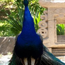
most of the attention components, as well as the parts of the         3.1. Relevance and gradients
networks that perform other types of computation. A self-
                                                                         Let C be the number of classes in the classification head,
attention head involves the computation of queries, keys,
                                                                      and t ∈ 1 . . . |C| the class to be visualized. We propagate
and values. Reducing it only to the obtained attention scores
                                                                      relevance and gradients with respect to class t, which is not
(inner products of queries and keys) is myopic. Other layers
                                                                      necessarily the predicted class. Following literature con-
are not even considered. Our method, in contrast, propa-
                                                                      vention, we denote x(n) as the input of layer L(n) , where
gates through all layers from the decision back to the input.
                                                                      n ∈ [1 . . . N ] is the layer index in a network that consists of
    LRP was applied for Transformers based on the premise             N layers, x(N ) is the input to the network, and x(1) is the
that considering mean attention heads is not optimal due to           output of the network.
different relevance of the attention heads in each layer [42].           Recalling the chain-rule, we propagate gradients with re-
However, this was done in a limiting way, in which no rel-            spect to the classifier’s output y, at class t, namely yt :
evance scores were propagated back to the input, thus pro-
viding partial information on the relevance of each head.                                             ∂yt                        ∂yt        ∂xi
                                                                                                                                                (n−1)
                                                                                     (n)
                                                                                                                  X
We note that the relevancy scores were not directly evalu-                       ∇xj         :=        (n)
                                                                                                              =                  (n−1)            (n)
                                                                                                                                                                  (1)
ated, only used for visualization of the relative importance                                      ∂xj               i       ∂xi              ∂xj
and for pruning less relevant attention heads.
                                                                      where the index j corresponds to elements in x(n) , and i
    The main challenge in assigning attributions based on at-
                                                                      corresponds to elements in x(n−1) .
tentions is that attentions are combining non-linearly from
                                                                         We denote by L(n) (X, Y) the layer’s operation on two
one layer to the next. The rollout method [1] assumes that
                                                                      tensors X and Y. Typically, the two tensors are the input
attentions are combined linearly and considers paths along
                                                                      feature map and weights for layer n. Relevance propagation
the pairwise attention graph. We observe that this method
                                                                      follows the generic Deep Taylor Decomposition [27]:
often leads to an emphasis on irrelevant tokens since even
average attention scores can be attenuated. The method                             (n)
                                                                                Rj       = G(X, Y, R(n−1) )                                                       (2)
also fails to distinguish between positive and negative con-
                                                                                                             (n)                       (n−1)
tributions to the decision. Without such a distinction, one                                  X             ∂Li (X, Y)                Ri
                                                                                         =            Xj                                                  ,
can mix between the two and obtain high relevancy scores,                                                         ∂Xj               (n)
                                                                                                                                   Li (X, Y)
                                                                                              i
when the contributions should have cancelled out. Despite
these shortcomings, the method was already applied by oth-            where, similarly to Eq. 1, the index j corresponds to ele-
ers [11] to obtain integrated attention maps.                         ments in R(n) , and i corresponds to elements in R(n−1) .
    Abnar et al. [1] present, in addition to rollout, a sec-          Eq. 2 satisfies the conservation rule [27], i.e.:
ond method called attention flow. The latter considers the                                X (n) X (n−1)
max-flow problem along the pair-wise attention graph. It                                     Rj =         Ri                 (3)
is shown to be sometimes more correlated than the rollout                                         j                     i
method with relevance scores that are obtained by applying
                                                                      LRP [2] assumes ReLU non-linearity activations, resulting
masking, or with gradients with respect to the input. This
                                                                      in non-negative feature maps, where the relevance propaga-
method is much slower and we did not evaluate it in our
                                                                      tion rule can be defined as follows:
experiments for computational reasons.
    We note this concurrent work [1] did not perform an                   (n)
                                                                                                                            X          x+  +
                                                                                                                                        j wji                 (n−1)
evaluation on benchmarks (for either rollout or attention-              Rj      = G(x+ , w+ , R(n−1) ) =                                                  Ri
                                                                                                                                            x+    +
                                                                                                                                  P
                                                                                                                             i         j0    j 0 wj 0 i
flow) in which relevancy is assigned in a way that is in-
                                                                                                                                                                  (4)
dependent of the BERT [9] network, for which the methods
were employed. There was also no comparison to relevancy              where X = x and Y = w are the layer’s input and weights.
assignment methods, other than the raw attention scores.              The superscript denotes the operation max(0, v) as v + .
                                                                         Non-linearities other that ReLU, such as GELU [18],
3. Method                                                             output both positive and negative values. To address this,
                                                                      LRP propagation in Eq. 4 can be modified by constructing
   The method employs LRP-based relevance to compute                  a subset of indices q = {(i, j)|xj wji ≥ 0}, resulting in the
scores for each attention head in each layer of a Transformer         following relevance propagation:
model [41]. It then integrates these scores throughout the at-
                                                                             (n)
tention graph, by incorporating both relevancy and gradient               Rj       = Gq (x, w, q, R(n−1) )
information, in a way that iteratively removes the negative                             X              xj wji                                     (n−1)
contributions. The result is a class-specific visualization for                    =            P                                               Ri                (5)
                                                                                                             {j 0 |(j 0 ,i)∈q}    xj 0 wj 0 i
self-attention models.                                                               {i|(i,j)∈q}

                                                                  3
In other words, we consider only the elements that have a wherePa and bP are large positive numbers. It is easy to verify
that Ru + Rv = ea + 1 − ea + eb + 1 − eb =
P
positive weighed relevance. R.
To initialize the relevance propagation, we set R(0) = 1t , As can be seen, while the conservation rule is preserved, the
where 1t is a one-hot indicating the target class t. relevance scores of u and v may explode. See supplemen-
tary for a step by step computation.
3.2. Non parametric relevance propagation: To address the lack of conservation in the attention
There are two operators in Transformer models that in- mechanism due to matrix multiplication, and the numerical
volve mixing of two feature map tensors (as opposed to a issues of the skip connections, our method applies a nor-
(n) (n)
feature map with a learned tensor): skip connections and malization to Rju and Rkv :
matrix multiplications (e.g. in attention modules). The two
operators require the propagation of relevance through both (n)
Rju
P P (n−1)
input tensors. Note that the two tensors may be of different (n) (n) j R
shapes in the case of matrix multiplication. R̄ju = Rju · Pi i u(n)
j Rj
(n) P v(n)
Rju
P
Given two tensors u and v, we compute the relevance j + k Rk
propagation of these binary operators (i.e., operators that P v(n)
k Rk
P (n−1)
process two operands), as follows: (n) (n) R
R̄kv = Rkv · Pi i v(n)
k Rk
P u(n) P v(n)
(n) (n)
j Rj + k Rk
Rju = G(u, v, R(n−1) ), Rkv = G(v, u, R(n−1) ) (6)
(n) (n) Following the conservation rule (Eq. 3), and the initial
where Rju and Rkv are the relevances for u and v re- P (n)
spectively. These operations yield both positive and nega- relevance, we obtain i Ri = 1 for each layer n.
tive values. The following lemma presents the properties of the nor-
The following lemma shows that for the case of addition, malized relevancy scores.
the conservation rule is preserved, i.e., Lemma 2. The normalization technique upholds the fol-
X (n) X (n) X (n−1) lowing properties: (i) it maintains the conservation rule,
Rju + Rkv = Ri . (7) (n) (n) P (n−1)
i.e.: j R̄ju + k R̄kv = i Ri
P P
j k i
, (ii) it bounds the
relevance sum of each tensor such that:
However, this is not the case for matrix multiplication. X (n) X (n) X (n−1)
Lemma 1. Given two tensors u and v, consider the rele- 0≤ R̄ju , R̄kv ≤ Ri (10)
j k i
vances that are computed according to Eq. 1. Then, (i) if
layer L(n) adds the two tensors, i.e., L(n) (u, v) = u + v Proof. See supplementary.
then the conservation rule of Eq. 2 is maintained. (ii) if the
layer performs matrix multiplication L(n) (u, v) = uv, then 3.3. Relevance and gradient diffusion
Eq. 2 does not hold in general.
Let M be a Transformer model consisting of B blocks,
Proof. (i) and (ii) are obtained from the output derivative of where each block b is composed of self-attention, skip con-
L(n) with respect to X. In an add layer, u and v are inde- nections, and additional linear and normalization layers in
pendent of each other, while in matrix multiplication they a certain assembly. The model takes as an input a sequence
are connected. A detailed proof of Lemma 3 is available in of s tokens, each of dimension d, with a special token for
the supplementary. classification, commonly identified as the token [CLS]. M
outputs a classification probability vector y of length C,
When propagating relevance of skip connections, we en- computed using the classification token. The self-attention
counter numerical instabilities. This arises despite the fact module operates on a small sub-space dh of the embedding
that, by the conservation rule of the addition operator, the dimension d, where h is the number of “heads”, such that
sum of relevance scores is constant. The underlying reason hdh = d. The self-attention module is defined as follows:
is that the relevance scores tend to obtain large absolute val-
ues, due to the way they are computed (Eq. 2). To see this, T
(b) Q(b) · K(b)
consider the following example: A = sof tmax( √ ) (11)
dh
a
1 − ea
e 1 O(b) = A(b) · V(b) (12)
u= , v = , R = (8)
eb 1 − eb 1
ea where (·) denotes matrix multiplication, O(b) ∈ Rh×s×dh
!
ea −ea +1 1 ea 1 − ea
u v
R = b = , R = (9) is the output of the attention module in block b,
e
1 eb 1 − eb
eb −eb +1 Q(b) , K(b) , V(b) ∈ Rh×s×dh are the query key and value
4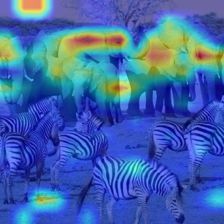
inputs in block b, namely, different projections of an input
x(n) for a self-attention module. A(b) ∈ Rh×s×s is the at-                                   Transformer
                                                                                                                      Gradients
                                                                                                                                  Transformer
                                                                                     Input                                                      Output
tention map of block b, where row i represents the attention                                    Block
                                                                                                                      Relevance
                                                                                                                                     Block

coefficients of each token in the input with respect to the to-                                Attetion

ken i. The sof tmax in Eq. 11 is applied, such that the sum
of each row in each attention head of A(b) is one.
   Following the propagation procedure of relevance and
gradients, each attention map A(b) has its gradients ∇A(b) ,                  Figure 1: Illustration of our method. Gradients and relevan-
and relevance R(nb ) , with respect to a target class t, where                cies are propagated through the network, and integrated to
nb is the layer that corresponds to the sof tmax operation                    produce the final relevancy maps, as described in Eq. 13, 14.
in Eq. 11 of block b, and R(nb ) is the layer’s relevance.
   The final output C ∈ Rs×s of our method is then defined
by the weighted attention relevance:                                          4. Experiments
             Ā(b) = I + Eh (∇A(b)                 R(nb ) )+       (13)           For the linguistic classification task, we experiment with
                        (1)          (2)                  (B)                 the BERT-base [9] model as our classifier, assuming a max-
                C = Ā        · Ā         · . . . · Ā            (14)
                                                                              imum of 512 tokens, and a classification token [CLS] that
where      is the Hadamard product, and Eh is the mean                        is used as the input to the classification head.
across the “heads” dimension. In order to compute the                             For the visual classification task, we experiment with the
weighted attention relevance, we consider only the positive                   pretrained ViT-base [11] model, which consists of a BERT-
values of the gradients-relevance multiplication, resembling                  like model. The input is a sequence of all non-overlapping
positive relevance. To account for the skip connections in                    patches of size 16 × 16 of the input image, followed by flat-
the Transformer block, we add the identity matrix to avoid                    tening and linear layers, to produce a sequence of vectors.
self inhibition for each token.                                               Similar to BERT, a classification token [CLS] is appended
   For comparison, using the same notation, the rollout [1]                   at the beginning of the sequence and used for classification.
method is given by:                                                               The baselines are divided into three classes: attention-
               Â(b) = I + Eh A(b)                                 (15)       maps, relevance, and gradient-based methods. Each has dif-
                            (1)        (2)                   (B)
                                                                              ferent properties and assumptions over the architecture and
             rollout = Â         · Â        · . . . · Â         (16)       propagation of information in the network. To best reflect
We can observe that the result of rollout is fixed given an                   the performance of different baselines, we focus on methods
input sample, regardless of the target class to be visualized.                that are both common in the explainability literature, and
In addition, it does not consider any signal, except for the                  applicable to the extensive tests we report in this section,
pairwise attention scores.                                                    e.g. Black-box methods, such as Perturbation and Shapely
                                                                              based methods, are computationally too expensive and in-
3.4. Obtaining the image relevance map                                        herently different from the proposed method. We briefly
    The resulting explanation of our method is a matrix C of                  describe each baseline in the following section and the dif-
size s × s, where s represents the sequence length of the in-                 ferent experiments for each domain.
put fed to the Transformer. Each row corresponds to a rele-                       The attention-map baselines include rollout [1], follow-
vance map for each token given the other tokens - following                   ing Eq. 16, which produces an explanation that takes into
the attention computation convention in Eq. 14, 11. Since                     account all the attention-maps computed along the forward-
this work focuses on classification models, only the [CLS]                    pass. A more straightforward method is raw attention, i.e.
token, which encapsulates the explanation of the classifica-                  using the attention map of block 1 to extract the relevance
tion, is considered. The relevance map is, therefore, derived                 scores. These methods are class-agnostic by definition.
from the row C[CLS] ∈ Rs that corresponds to the [CLS]                            Unlike attention-map based methods, the relevance prop-
token. This row contains a score evaluating each token’s                      agation methods consider the information flow through the
influence on the classification token.                                        entire network, and not just the attention maps. These base-
    We consider only the tokens that correspond to the ac-                    lines include Eq. 4 and the partial application of LRP that
tual input, without special tokens, such as the [CLS] token                   follows [42]. As we show in our experiments, the different
and other separators. In vision models, such as ViT [11],                     variants of the LRP method are practically class-agnostic,
the content tokens represent image patches. To obtain the                     meaning the visualization remains approximately the same
final relevance map, we reshape the sequence to the patches                   for different target classes.
grid size, √
√           e.g. for a square image, the patch grid size is                       A common class-specific explanation method is Grad-
   s − 1 × s − 1. This map is upsampled back to the size                      CAM [32], which computes a weighted gradient-feature-
of the original image using bilinear interpolation.                           map to the last convolution layer in a CNN model. The best

                                                                          5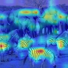
way we found to apply GradCAM was to treat the last at-              ERASER [10] for rationales extraction, where the goal is
tention layer’s [CLS] token as the designated feature map,           to extract parts of the input that support the (ground truth)
without considering the [CLS] token itself. We note that             classification. The BERT model is first fine-tuned on the
the last output of a Transformer model (before the classifi-         training set of the Movie Reviews Dataset and the various
cation head), is a tensor v ∈ Rs×d , where the first dimension       evaluation methods are applied to its results on the test set.
relates to different input tokens, and only the [CLS] token          We report the token-F1 score, which is best suited for per-
is fed to the classification head. Thus, performing Grad-            token explanation (in contrast to explanations that extract an
CAM on v will impose a sparse gradients tensor ∇v, with              excerpt). To best illustrate the performance of each method,
zeros for all tokens, except [CLS].                                  we consider a token to be part of the “rationale” if it is part
Evaluation settings For the visual domain, we follow                 of the top-k tokens, and show results for k = 10 . . . 80 in
the convention of reporting results for negative and pos-            steps of 10 tokens. This way, we do not employ threshold-
itive perturbations, as well as showing results for seg-             ing that may benefit some methods over others.
mentation, which can be seen as a general case of ”The               4.1. Results
Pointing-Game” [19]. The dataset used is the validation
set of ImageNet [31] (ILSVRC) 2012, consisting of 50K                Qualitative evaluation Fig.2 presents a visual comparison
images from 1000 classes, and an annotated subset of                 between our method and the various baselines. As can
ImageNet called ImageNet-Segmentation [16], containing               be seen, the baseline methods produce inconsistent perfor-
4,276 images from 445 categories. For the linguistic do-             mance, while our method results in a much clearer and con-
main, we follow ERASER [10] and evaluate the reason-                 sistent visualization.
ing for the Movies Reviews [44] dataset, which consists of               In order to show that our method is class-specific, we
1600/200/200 reviews for train/val/test. This task is a binary       show in Fig. 3 images with two objects, each from a dif-
sentiment analysis task. Providing explanations for ques-            ferent class. As can be seen, all methods, except Grad-
tion answering and entailment tasks of the other datasets in         CAM, produce similar visualization for each class, while
ERASER, which require input sizes of more than 512 to-               our method provides two different and accurate visualiza-
kens (the limit of our BERT model), is left for future work.         tions.
    The positive and negative perturbation tests follow a two-       Perturbation tests Tab. 1 presents the AUC obtained for
stage setting. First, a pre-trained network is used for ex-          both negative and positive perturbation tests, for both the
tracting visualizations for the validation set of ImageNet.          predicted and the target class. As can be seen, our method
Second, we gradually mask out the pixels of the input im-            achieves better performance by a large margin in both tests.
age and measure the mean top-1 accuracy of the network.              Notice that because rollout and raw attention produce con-
In positive perturbation, pixels are masked from the high-           stant visualization given an input image, we omit their
est relevance to the lowest, while in the negative version,          scores in the target-class test.
from lowest to highest. In positive perturbation, one ex-
                                                                     Segmentation The segmentation metrics (pixel-accuracy,
pects to see a steep decrease in performance, which indi-
                                                                     mAP, and mIoU) on ImageNet-segmentation are shown in
cates that the masked pixels are important to the classifi-
                                                                     Tab. 2. As can be seen, our method outperforms all base-
cation score. In negative perturbation, a good explanation
                                                                     lines by a significant margin.
would maintain the accuracy of the model, while remov-
ing pixels that are not related to the class. In both cases,         Language reasoning Fig. 4 depicts the performance on the
we measure the area-under-the-curve (AUC), for erasing be-           Movie Reviews “rationales” experiment, evaluating for top-
tween 10% − 90% of the pixels.                                       K tokens, ranging from 10 to 80. As can be seen, while
    The two tests can be applied to the predicted or the             all methods benefit from increasing the amount tokens, our
ground-truth class. Class-specific methods are expected to           method consistently outperforms the baselines. See supple-
gain performance in the latter case, while class-agnostic            mentary for a depiction of the obtained visualization.
methods would present similar performance in both tests.             Ablation study. We consider three variants of our method
    The segmentation tests consider each visualization as            and present their performance on the segmentation and pre-
a soft-segmentation of the image, and compare it to the              dicted class perturbation experiments. (i) Ours w/o ∇A(b) ,
ground truth segmentation of the ImageNet-Segmentation               which modifies Eq. 13 s.t. we use A(b) instead of ∇A(b) ,
dataset. Performance is measured by (i) pixel-accuracy,              (ii) ∇A(1) R(n1 ) , i.e. disregarding rollout in Eq. 14, and us-
obtained after thresholding each visualization by the                ing our method only on block 1, which is the block closest
mean value, (ii) mean-intersection-over-union (mIoU), and            to the output, and (iii) ∇A(B−1) R(nB−1 ) which similar to
(iii) mean-Average-Precision (mAP), which uses the soft-             (ii), only for block B − 1 which is closer to the input.
segmentation to obtain a score that is threshold-agnostic.               As can be seen in Tab. 3 the ablation ∇A(1) R(n1 ) in
    The NLP benchmark follows the evaluation setting of              which one removes the rollout component, i.e., Eq. 14,

                                                                 6
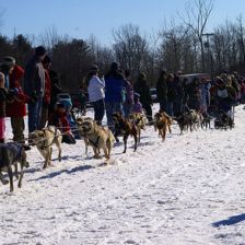
Input          rollout [1]     raw-attention    GradCAM [32]         LRP [3]       partial LRP [42]        Ours

               Figure 2: Sample results. As can be seen, our method produces more accurate visualizations.

     Input          rollout [1]     raw-attention   GradCAM [32]         LRP [3]       partial LRP [42]        Ours

    Dog →

    Cat →

  Elephant →

   Zebra →

Figure 3: Class-specific visualizations. For each image we present results for two different classes. GradCam is the only
method to generate different maps. However, its results are not convincing.

                                                           7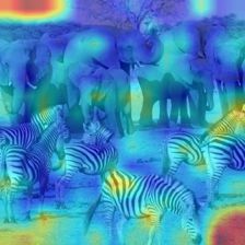
rollout [1]            raw attention      GradCAM [32]          LRP [3]       partial LRP [42]      Ours
                       Predicted             53.1               45.55                41.52             43.49             50.49            54.16
Negative
                       Target                 -                   -                  42.02             43.49             50.49            55.04
                       Predicted         20.05                  23.99                34.06             41.94             19.64            17.03
Positive
                       Target              -                      -                  33.56             41.93             19.64            16.04

Table 1: Positive and Negative perturbation AUC results (percents) for the predicted and target classes, on the ImageNet [31]
validation set. For positive perturbation lower is better, and for negative perturbation higher is better.

                              rollout [1]            raw attention           GradCAM [32]          LRP [3]        partial LRP [42]        Ours
pixel accuracy                  73.54                   67.84                   64.44               51.09               76.31             79.70
mAP                             84.76                   80.24                   71.60               55.68               84.67             86.03
mIoU                            55.42                   46.37                   40.82               32.89               57.94             61.95

              Table 2: Segmentation performance on the ImageNet-segmentation [16] dataset (percent). Higher is better.

           0.25          Ours                                                       methods, indicating that the advantage of our method stems
                         partial LRP                                                mostly from the combination of relevancy as we compute it
           0.20          raw attention                                              and attention-map gradients.
                         GradCAM
           0.15
token-F1

                         LRP                                                        5. Conclusions
                         rollout
           0.10                                                                         The self-attention mechanism links each of the tokens to
                                                                                    the [CLS] token. The strength of this attention link can
           0.05                                                                     be intuitively considered as an indicator of the contribution
                                                                                    of each token to the classification. While this is intuitive,
           0.00                                                                     given the term “attention”, the attention values reflect only
                  10     20     30      40      50      60      70    80
                                     # of Tokens                                    one aspect of the Transformer network or even of the self-
                                                                                    attention head. As we demonstrate, both when using a fine-
Figure 4: token-F1 scores on the Movie Reviews reasoning                            tuned BERT model for NLP and with the ViT model, atten-
task.                                                                               tions lead to fragmented and non-competitive explanations.
                                                                                        Despite this shortcoming and the importance of Trans-
                                   Segmentation              Perturbations          former models, the literature with regards to interpretability
                               Acc. mAP mIoU Pos.                    Neg.           of Transformers is sparse. In comparison to CNNs, multiple
                                                                                    factors prevent methods developed for other forms of neu-
Ours w/o ∇A(b)                77.66   85.66         59.88   18.23    52.88          ral networks (not including the slower black-box methods)
∇A(1) R(n1 )                  78.32   85.25         59.93   18.01    52.43          from being applied. These include the use of non-positive
∇A(B−1) R(nB−1 )              60.30   73.63         39.06   27.33    37.42          activation functions, the frequent use of skip connections,
Ours                          79.70   86.03         61.95   17.03    54.16          and the challenge of modeling the matrix multiplication that
                                                                                    is used in self-attention.
 Table 3: Performance of different variants of our method.                              Our method provides specific solutions to each of these
                                                                                    challenges and obtains state-of-the-art results when com-
                                                                                    pared to the methods of the Transformer literature, the LRP
while keeping the relevance and gradient integration, and                           method, and the GradCam method, which can be applied
only considering the last attention layer, leads to a moder-                        directly to Transformers.
ate drop in performance. Out of the two single block vi-
sualizations ((ii), and (iii)), the combined attention gradient                     Acknowledgment
and relevancy at the b = 1 block, which is the closest to
the output, is more informative than the block closest to the                          This project has received funding from the European Re-
input. This is the same block that is being used for the raw-                       search Council (ERC) under the European Unions Horizon
attention, partial LRP, and the GradCAM methods. The                                2020 research and innovation programme (grant ERC CoG
ablation that considers only this block outperforms these                           725974). The contribution of the first author is part of a

                                                                                8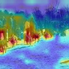
Master thesis research conducted at Tel Aviv University.                        smooth masks. In Proceedings of the IEEE International
                                                                                Conference on Computer Vision, pages 2950–2958, 2019. 2
References                                                               [14]   Ruth C Fong and Andrea Vedaldi. Interpretable explanations
                                                                                of black boxes by meaningful perturbation. In Proceedings
 [1] Samira Abnar and Willem Zuidema. Quantifying atten-                        of the IEEE International Conference on Computer Vision,
     tion flow in transformers. arXiv preprint arXiv:2005.00928,                pages 3429–3437, 2017. 2
     2020. 1, 3, 5, 7, 8                                                 [15]   Jindong Gu, Yinchong Yang, and Volker Tresp. Understand-
 [2] Sebastian Bach, Alexander Binder, Grégoire Montavon,                      ing individual decisions of cnns via contrastive backpropaga-
     Frederick Klauschen, Klaus-Robert Müller, and Wojciech                    tion. In Asian Conference on Computer Vision, pages 119–
     Samek. On pixel-wise explanations for non-linear classi-                   134. Springer, 2018. 2
     fier decisions by layer-wise relevance propagation. PloS one,       [16]   Matthieu Guillaumin, Daniel Küttel, and Vittorio Ferrari.
     10(7):e0130140, 2015. 2, 3                                                 Imagenet auto-annotation with segmentation propagation.
 [3] Alexander Binder, Grégoire Montavon, Sebastian La-                        International Journal of Computer Vision, 110(3):328–348,
     puschkin, Klaus-Robert Müller, and Wojciech Samek.                        2014. 6, 8
     Layer-wise relevance propagation for neural networks with           [17]   Shir Gur, Ameen Ali, and Lior Wolf. Visualization of su-
     local renormalization layers. In International Conference on               pervised and self-supervised neural networks via attribution
     Artificial Neural Networks, pages 63–71. Springer, 2016. 1,                guided factorization. In AAAI, 2021. 2
     7, 8                                                                [18]   Dan Hendrycks and Kevin Gimpel. Gaussian error linear
 [4] Nicolas Carion, Francisco Massa, Gabriel Synnaeve, Nicolas                 units (gelus). arXiv preprint arXiv:1606.08415, 2016. 3
     Usunier, Alexander Kirillov, and Sergey Zagoruyko. End-             [19]   Sara Hooker, Dumitru Erhan, Pieter-Jan Kindermans, and
     to-end object detection with transformers. arXiv preprint                  Been Kim. A benchmark for interpretability methods in deep
     arXiv:2005.12872, 2020. 1                                                  neural networks. In Advances in Neural Information Pro-
 [5] Jianbo Chen, Le Song, Martin J. Wainwright, and Michael I.                 cessing Systems, pages 9737–9748, 2019. 6
     Jordan. L-shapley and c-shapley: Efficient model interpre-          [20]   Brian Kenji Iwana, Ryohei Kuroki, and Seiichi Uchida.
     tation for structured data. In International Conference on                 Explaining convolutional neural networks using softmax
     Learning Representations, 2019. 2                                          gradient layer-wise relevance propagation. arXiv preprint
 [6] Mark Chen, Alec Radford, Rewon Child, Jeff Wu, Hee-                        arXiv:1908.04351, 2019. 2
     woo Jun, Prafulla Dhariwal, David Luan, and Ilya Sutskever.         [21]   Kunpeng Li, Ziyan Wu, Kuan-Chuan Peng, Jan Ernst, and
     Generative pretraining from pixels. In Proceedings of the                  Yun Fu. Tell me where to look: Guided attention inference
     37th International Conference on Machine Learning, vol-                    network. In Proceedings of the IEEE Conference on Com-
     ume 1, 2020. 1                                                             puter Vision and Pattern Recognition, pages 9215–9223,
 [7] Jianpeng Cheng, Li Dong, and Mirella Lapata. Long short-                   2018. 2
     term memory-networks for machine reading. In Proceedings            [22]   Yinhan Liu, Myle Ott, Naman Goyal, Jingfei Du, Man-
     of the 2016 Conference on Empirical Methods in Natural                     dar Joshi, Danqi Chen, Omer Levy, Mike Lewis, Luke
     Language Processing, pages 551–561, 2016. 1                                Zettlemoyer, and Veselin Stoyanov. RoBERTa: A ro-
 [8] Piotr Dabkowski and Yarin Gal. Real time image saliency                    bustly optimized bert pretraining approach. arXiv preprint
     for black box classifiers. In Advances in Neural Information               arXiv:1907.11692, 2019. 1
     Processing Systems, pages 6970–6979, 2017. 2                        [23]   Jiasen Lu, Dhruv Batra, Devi Parikh, and Stefan Lee. Vil-
 [9] Jacob Devlin, Ming-Wei Chang, Kenton Lee, and Kristina                     bert: Pretraining task-agnostic visiolinguistic representations
     Toutanova.       Bert: Pre-training of deep bidirectional                  for vision-and-language tasks. In Advances in Neural Infor-
     transformers for language understanding. arXiv preprint                    mation Processing Systems, pages 13–23, 2019. 1
     arXiv:1810.04805, 2018. 1, 3, 5                                     [24]   Scott M Lundberg and Su-In Lee. A unified approach to
[10] Jay DeYoung, Sarthak Jain, Nazneen Fatema Rajani, Eric                     interpreting model predictions. In Advances in Neural Infor-
     Lehman, Caiming Xiong, Richard Socher, and Byron C Wal-                    mation Processing Systems, pages 4765–4774, 2017. 2
     lace. Eraser: A benchmark to evaluate rationalized nlp mod-         [25]   Aravindh Mahendran and Andrea Vedaldi. Visualizing deep
     els. arXiv preprint arXiv:1911.03429, 2019. 2, 6                           convolutional neural networks using natural pre-images. In-
[11] Alexey Dosovitskiy, Lucas Beyer, Alexander Kolesnikov,                     ternational Journal of Computer Vision, 120(3):233–255,
     Dirk Weissenborn, Xiaohua Zhai, Thomas Unterthiner,                        2016. 2
     Mostafa Dehghani, Matthias Minderer, Georg Heigold, Syl-            [26]   Brent Mittelstadt, Chris Russell, and Sandra Wachter. Ex-
     vain Gelly, et al. An image is worth 16x16 words: Trans-                   plaining explanations in ai. In Proceedings of the conference
     formers for image recognition at scale. arXiv preprint                     on fairness, accountability, and transparency, pages 279–
     arXiv:2010.11929, 2020. 1, 3, 5                                            288, 2019. 2
[12] Dumitru Erhan, Yoshua Bengio, Aaron Courville, and Pascal           [27]   Grégoire Montavon, Sebastian Lapuschkin, Alexander
     Vincent. Visualizing higher-layer features of a deep network.              Binder, Wojciech Samek, and Klaus-Robert Müller. Ex-
     University of Montreal, 1341(3):1, 2009. 2                                 plaining nonlinear classification decisions with deep taylor
[13] Ruth Fong, Mandela Patrick, and Andrea Vedaldi. Un-                        decomposition. Pattern Recognition, 65:211–222, 2017. 1,
     derstanding deep networks via extremal perturbations and                   2, 3

                                                                     9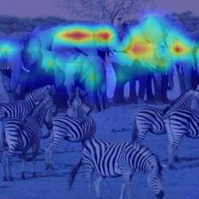
[28] Woo-Jeoung Nam, Shir Gur, Jaesik Choi, Lior Wolf, and                       Polosukhin. Attention is all you need. In Advances in neural
     Seong-Whan Lee. Relative attributing propagation: Inter-                    information processing systems, pages 5998–6008, 2017. 1,
     preting the comparative contributions of individual units in                3
     deep neural networks. arXiv preprint arXiv:1904.00605,               [42]   Elena Voita, David Talbot, Fedor Moiseev, Rico Sennrich,
     2019. 2                                                                     and Ivan Titov. Analyzing multi-head self-attention: Spe-
[29] Ankur Parikh, Oscar Täckström, Dipanjan Das, and Jakob                    cialized heads do the heavy lifting, the rest can be pruned. In
     Uszkoreit. A decomposable attention model for natural lan-                  Proceedings of the 57th Annual Meeting of the Association
     guage inference. In Proceedings of the 2016 Conference on                   for Computational Linguistics, pages 5797–5808, 2019. 1,
     Empirical Methods in Natural Language Processing, pages                     3, 5, 7, 8
     2249–2255, 2016. 1                                                   [43]   Kelvin Xu, Jimmy Ba, Ryan Kiros, Kyunghyun Cho, Aaron
[30] Alec Radford, Jeff Wu, Rewon Child, David Luan, Dario                       Courville, Ruslan Salakhudinov, Rich Zemel, and Yoshua
     Amodei, and Ilya Sutskever. Language models are unsuper-                    Bengio. Show, attend and tell: Neural image caption gen-
     vised multitask learners. 2019. 1                                           eration with visual attention. In International conference on
[31] Olga Russakovsky, Jia Deng, Hao Su, Jonathan Krause, San-                   machine learning, pages 2048–2057, 2015. 1
     jeev Satheesh, Sean Ma, Zhiheng Huang, Andrej Karpathy,              [44]   Omar Zaidan and Jason Eisner. Modeling annotators: A gen-
     Aditya Khosla, Michael Bernstein, et al. Imagenet large                     erative approach to learning from annotator rationales. In
     scale visual recognition challenge. International journal of                Proceedings of the 2008 conference on Empirical methods
     computer vision, 115(3):211–252, 2015. 6, 8                                 in natural language processing, pages 31–40, 2008. 6
[32] Ramprasaath R Selvaraju, Michael Cogswell, Abhishek Das,             [45]   Matthew D Zeiler and Rob Fergus. Visualizing and under-
     Ramakrishna Vedantam, Devi Parikh, and Dhruv Batra.                         standing convolutional networks. In European conference on
     Grad-cam: Visual explanations from deep networks via                        computer vision, pages 818–833. Springer, 2014. 2
     gradient-based localization. In Proceedings of the IEEE in-          [46]   Jianming Zhang, Sarah Adel Bargal, Zhe Lin, Jonathan
     ternational conference on computer vision, pages 618–626,                   Brandt, Xiaohui Shen, and Stan Sclaroff. Top-down neu-
     2017. 2, 5, 7, 8                                                            ral attention by excitation backprop. International Journal
[33] Avanti Shrikumar, Peyton Greenside, and Anshul Kundaje.                     of Computer Vision, 126(10):1084–1102, 2018. 2
     Learning important features through propagating activation           [47]   Bolei Zhou, David Bau, Aude Oliva, and Antonio Torralba.
     differences. In Proceedings of the 34th International Con-                  Interpreting deep visual representations via network dissec-
     ference on Machine Learning-Volume 70, pages 3145–3153.                     tion. IEEE transactions on pattern analysis and machine
     JMLR. org, 2017. 2                                                          intelligence, 2018. 2
[34] Avanti Shrikumar, Peyton Greenside, Anna Shcherbina, and             [48]   Bolei Zhou, Aditya Khosla, Agata Lapedriza, Aude Oliva,
     Anshul Kundaje. Not just a black box: Learning important                    and Antonio Torralba. Learning deep features for discrimina-
     features through propagating activation differences. arXiv                  tive localization. In Proceedings of the IEEE conference on
     preprint arXiv:1605.01713, 2016. 2                                          computer vision and pattern recognition, pages 2921–2929,
[35] Karen Simonyan, Andrea Vedaldi, and Andrew Zisserman.                       2016. 2
     Deep inside convolutional networks: Visualising image
     classification models and saliency maps. arXiv preprint
     arXiv:1312.6034, 2013. 2
[36] Daniel Smilkov, Nikhil Thorat, Been Kim, Fernanda Viégas,
     and Martin Wattenberg. Smoothgrad: removing noise by
     adding noise. arXiv preprint arXiv:1706.03825, 2017. 2
[37] Suraj Srinivas and François Fleuret. Full-gradient repre-
     sentation for neural network visualization. In Advances in
     Neural Information Processing Systems, pages 4126–4135,
     2019. 2
[38] Weijie Su, Xizhou Zhu, Yue Cao, Bin Li, Lewei Lu, Furu
     Wei, and Jifeng Dai. Vl-bert: Pre-training of generic visual-
     linguistic representations. arXiv preprint arXiv:1908.08530,
     2019. 1
[39] Mukund Sundararajan, Ankur Taly, and Qiqi Yan. Axiomatic
     attribution for deep networks. In Proceedings of the 34th
     International Conference on Machine Learning-Volume 70,
     pages 3319–3328. JMLR. org, 2017. 2
[40] Hao Tan and Mohit Bansal. Lxmert: Learning cross-
     modality encoder representations from transformers. arXiv
     preprint arXiv:1908.07490, 2019. 1
[41] Ashish Vaswani, Noam Shazeer, Niki Parmar, Jakob Uszko-
     reit, Llion Jones, Aidan N Gomez, Łukasz Kaiser, and Illia

                                                                     10
A. Details of the various Baselines
GradCAM As mentioned in Sec. 4, we consider the last attention layer (closest to the output) - namely A(1) . This results
in a feature-map of size h × s × s. Following the process described in Sec. 3.4, we take only the [CLS] token’s row (without
the [CLS] token’s column), and reshape to the patches grid size hp × wp . This results in a feature-map similar to the 2D
feature-map used for GradCAM, where the number of channels, in this case, is h, and the height and width are hp and wp .
The reason we use the last attention layer is because of the sparse gradients issue described in Sec. 4.
raw-attention The raw-attention method visualizes the last attention layer (closest to the output) - namely A(1) . It follows
the process described in Sec. 3.4 to extract the final output.
LRP In this method, we propagate relevance up to the input image, following the propagation rules of LRP (not our
modified rules and normalizations).
partial-LRP Following [42], we visualize an intermediate relevance map, more specifically, we visualize the last attention-
map’s relevance, namely R(n1 ) , using LRP propagation rules.
rollout We follow Eq. 16.
11B. Proofs for Lemmas
Given two tensors u and v, we compute the relevance propagation of binary operators (i.e., operators that process two
operands) as follows:
(n)
Rju = G(u, v, R(n−1) )
(n)
Rkv = G(v, u, R(n−1) ) (1)
(n) (n)
where Rju and Rkv are the relevances for u and v respectively.
The following lemma shows that for the case of addition, the conservation rule is preserved, i.e.,
X (n) X (n) X (n−1)
Rju + Rkv = Ri . (2)
j k i
However, this is not the case for matrix multiplication.
Lemma 3. Given two tensors u and v, consider the relevances that are computed according to Eq. 1. Then, (i) if layer L(n)
adds the two tensors, i.e., L(n) (u, v) = u + v then the conservation rule of Eq. 2 is maintained. (ii) if the layer performs
matrix multiplication L(n) (u, v) = uv, then Eq. 2 does not hold in general.
Proof. For part (i), we note that the number of elements in u equals the number of elements in v, therefore k = j, and we
can write Eq. 2 following the definition of G:
(n−1) (n−1)
XX ∂(ui + vi ) Ri X X ∂(ui + vi ) R
i
uj + vj
j i
∂u j u i + v i j i
∂vj ui + vi
X uj (n−1)
X v j (n−1)
= Rj + Rj
j
uj + v j j
u j + v j
X uj + vj (n−1) X (n−1)
= R = Rj (3)
j
uj + vj j j
(n) (n)
Rju Rjv
P P
note that, in this case, it is possible that j 6= j .
As shown in the
main text, while
the sumoftwo tensors maintains the conservation rule, their values may explode.
ea 1 − ea 1
Consider u = ,v= and R = , following the definition of G we have:
eb 1 − eb 1
(n−1)
(n) X ∂(ui + vi ) Ri uj (n−1) (n) vj (n−1)
Rju = uj = Rj , Rjv = R
i
∂u j ui + v i u j + v j uj + vj j
ea
!
ea −ea +1 1 ea 1 − ea
u v
R = b = , R = (4)
e
eb −eb +1
1 eb 1 − eb
which causes numerical instability.
For part (ii), in the case of matrix multiplication between u and v, where u ∈ Rk,m , v ∈ Rm,l , we will show that:
12(n) (n) (n−1)
u v
P P P P P P
k m Rk,m = m l Rm,l = l k Rk,l , which invalidates the conservation rule:
(n−1)
(n) ∂(uv)k,l R u v
P k,l P k,m m,l Rk,l(n−1)
X X
u
Rk,m = uk,m = (5)
∂uk,m m0 uk,m vm l
0 0
m0 uk,m vm l
0 0
l l
(n−1)
v (n) ∂(uv)k,l Rk,l u v
P k,m m,l Rk,l (n−1)
X X
Rm,l = vm,l P = (6)
∂vm,l u 0
m0 k,m m l v 0 u 0
m0 k,m m lv 0
k k
(n) (n) uk,m vm,l u v
(n−1)
P k,m m,l Rk,l (n−1)
XX XX XXX XXX
u v
Rk,m + Rm,l = P Rk,l +
m m m
u 0
m0 k,m m lv 0
m
u 0
m0 k,m m l v 0
k l k l l k
X X P uk,m vm,l (n−1) X X P uk,m vm,l (n−1)
= Pm Rk,l + Pm Rk,l (7)
m0 uk,m0 vm0 l m0 uk,m vm l
0 0
k l l k
X X (n−1)
=2 Rk,l (8)
l k
To address the lack of conservation in the attention mechanism, which employs multiplication, and the numerical issues
(n) (n)
of the skip connections, our method applies a normalization to Rju and Rkv :
(n)
Rju
P P (n−1)
(n) (n) j R
R̄ju = Rju · Pi i u(n)
j Rj
(n) P v(n)
Rju
P
j + k Rk
P v(n)
k Rk
P (n−1)
(n) (n) R
R̄kv = Rkv · Pi i v(n) (9)
k Rk
P u(n) P v(n)
j Rj + k Rk
Lemma 4. The normalization technique upholds the following properties: (i) it maintains the conservation rule, i.e.:
P u(n) P v(n) P (n−1)
j R̄j + k R̄k = i Ri , (ii) it bounds the relevance sum of each tensor such that:
X (n) X (n) X (n−1)
0≤ R̄ju , R̄kv ≤ Ri (10)
j k i
Proof. For part (i), it holds that:
X (n) X (n)
R̄ju + R̄kv (11)
j k
(n)
Rju
P P (n−1)
X (n) j R
= Rju · Pi i u(n)
j Rj
(n) P v(n)
Rju
P
j + j k Rk
P v(n)
k Rk
P (n−1)
i Ri
X (n)
v
+ Rk P v(n) · P v(n) (12)
k Rk
P u(n)
k j Rj + k Rk
P u(n) P v(n)
j Rj X (n−1) k Rk X (n−1)
= P · R i + · Ri (13)
u(n) + v (n) u(n) + v (n)
P P P
R
j j R
k k i R
j j R
k k i
P u(n) P v(n)
j Rj + k Rk X (n−1) X (n−1)
= P (n) (n)
· Ri = Ri (14)
u v
P
j Rj + k Rk i i
13For part (ii) it is trivial to see that we weigh each tensor according to its relative absolute-value contribution:
(n)
Rju
P P (n−1)
X (n) X (n) j R
R̄ju = Rju · Pi i u(n) (15)
j Rj
(n) (n)
Rju Rkv
P P
j j j + k
(n)
Rju
P
j X (n−1)
= P · Ri (16)
u(n) v (n)
P
j Rj + k Rk i
we see that:
(n)
Rju
P
j
0≤ P (n) (n)
≤1 (17)
u v
P
j Rj + k Rk
therefore:
X (n) X (n) X (n−1)
0≤ R̄ju , R̄kv ≤ Ri (18)
j k i
14C. Visualizations - Multiple-class Images
Input rollout raw-attention GradCAM LRP partial LRP Ours
Dog →
Cat →
Elephant →
Zebra →
Elephant →
Zebra →
Elephant →
Zebra →
Figure 1: Multiple-class visualization. For each input image, we visualize two different classes. As can be seen, only our
method and GradCAM produce class-specific visualisations, where our method has fewer artifacts, and captures the objects
more completely.
15Input rollout raw-attention GradCAM LRP partial LRP Ours
Elephant →
Zebra →
Elephant →
Zebra →
Dog →
Cat →
Figure 2: Multiple-class visualization. For each input image, we visualize two different classes. As can be seen, only our
method and GradCAM produce class-specific visualisations, where our method has fewer artifacts, and captures the objects
more completely.
16D. Visualizations - Single-class Images
Input rollout raw-attention GradCAM LRP partial LRP Ours
Figure 3: Sample images from ImageNet val-set.
17Input rollout raw-attention GradCAM LRP partial LRP Ours
Figure 4: Sample images from ImageNet val-set.
18Input rollout raw-attention GradCAM LRP partial LRP Ours
Figure 5: Sample images from ImageNet val-set.
19Input rollout raw-attention GradCAM LRP partial LRP Ours
Figure 6: Sample images from ImageNet val-set.
20Input rollout raw-attention GradCAM LRP partial LRP Ours
Figure 7: Sample images from ImageNet val-set.
21Input rollout raw-attention GradCAM LRP partial LRP Ours
Figure 8: Sample images from ImageNet val-set.
22Input rollout raw-attention GradCAM LRP partial LRP Ours
Figure 9: Sample images from ImageNet val-set.
23Input rollout raw-attention GradCAM LRP partial LRP Ours
Figure 10: Sample images from ImageNet val-set.
24Input rollout raw-attention GradCAM LRP partial LRP Ours
Figure 11: Sample images from ImageNet val-set.
25Input rollout raw-attention GradCAM LRP partial LRP Ours
Figure 12: Sample images from ImageNet val-set.
26E. Visualizations - Text
In the following visualizations, we use the TAHV heatmap generator for text (https://github.com/jiesutd/
Text-Attention-Heatmap-Visualization) to present the relevancy scores for each method, as well as the ex-
cerpts marked by humans. For methods that are class-dependent, we present the attributions obtained both for the ground
truth class and the counter-factual class.
Evidently, our method is the only one that is able to present support for both sides, see panels (b,c) of each image.
GradCAM often suffers from highlighting the evidence in the opposite direction (sign reversal), e.g., Fig. 13(g), in which the
counter-factual explanation of GradCAM supports the negative, ground truth, sentiment and not the positive one.
Partial LRP (panels d,e) is not class-specific in practice. This provides it with an advantage in the quantitative experiments:
Partial LRP highlights words with both positive and negative connotations from the same sentence, which better matches the
behavior of the human annotators who are asked to mark complete sentences.
Notice that in most visualizations, it seems that the rollout method focuses mostly on the separation token [SEP], and fails
to generate meaningful visualizations. This corresponds to the results presented in the quantitative experiments.
It seems from our results, e.g., Fig. 13(b,c) that the BERT tokenizer leads to unintuitive results. For example, “joyless” is
broken down into “joy” and “less”, each supporting different sides of the decision.
27there may not be a critic alive who harbors as much affection for shlock monster movies [CLS] there may not be a critic alive who harbors as much affection for shlock monster [CLS] there may not be a critic alive who harbors as much affection for shlock monster
as i do . i delighted in the sneaky - smart entertainment of ron underwood ’s big - movies as i do . i delighted in the sneaky - smart entertainment of ron underwood ’ s big movies as i do . i delighted in the sneaky - smart entertainment of ron underwood ’ s big
underground - worm yarn tremors ; i even giggled at last year ’s critically - savaged big - - underground - worm yarn tremors ; i even giggled at last year ’ s critically - savaged big - underground - worm yarn tremors ; i even giggled at last year ’ s critically - savaged big
underwater - snake yarn anaconda . something about these films causes me to lower my - underwater - snake yarn anaconda . something about these films causes me to lower my - underwater - snake yarn anaconda . something about these films causes me to lower my
inhibitions and return to the saturday afternoons of my youth , spent in the company of inhibitions and return to the saturday afternoons of my youth , spent in the company of inhibitions and return to the saturday afternoons of my youth , spent in the company of
ghidrah , the creature from the black lagoon and the blob . deep rising , a big - undersea ghidrah , the creature from the black lagoon and the blob . deep rising , a big - undersea - ghidrah , the creature from the black lagoon and the blob . deep rising , a big - undersea -
- serpent yarn , does n’t quite pass the test . sure enough , all the modern monster movie serpent yarn , does n ’ t quite pass the test . sure enough , all the modern monster movie serpent yarn , does n ’ t quite pass the test . sure enough , all the modern monster movie
ingredients are in place : a conspicuously multi - ethnic / multi - national collection of ingredients are in place : a conspicuously multi - ethnic / multi - national collection of ingredients are in place : a conspicuously multi - ethnic / multi - national collection of
bait . .. excuse me , characters ; an isolated location , here a derelict cruise ship in the bait . . . excuse me , characters ; an isolated location , here a derelict cruise ship in the bait . . . excuse me , characters ; an isolated location , here a derelict cruise ship in the
south china sea ; some comic relief ; a few cgi - enhanced gross - outs ; and at least one south china sea ; some comic relief ; a few cgi - enhanced gross - outs ; and at least one south china sea ; some comic relief ; a few cgi - enhanced gross - outs ; and at least one
big explosion . there are too - cheesy - to - be - accidental elements , like a sleazy shipping big explosion . there are too - cheesy - to - be - accidental elements , like a sleazy shipping big explosion . there are too - cheesy - to - be - accidental elements , like a sleazy shipping
magnate ( anthony heald ) who also appears to have a doctorate in marine biology , or magnate ( anthony heald ) who also appears to have a doctorate in marine biology , or magnate ( anthony heald ) who also appears to have a doctorate in marine biology , or
a slinky international jewel thief ( famke janssen ) whose white cotton tank top hides a slinky international jewel thief ( famke janssen ) whose white cotton tank top hides a slinky international jewel thief ( famke janssen ) whose white cotton tank top hides
a heart of gold . as it happens , deep rising is noteworthy primarily for the mechanical a heart of gold . as it happens , deep rising is noteworthy primarily for the mechanical a heart of gold . as it happens , deep rising is noteworthy primarily for the mechanical
manner in which it spits out all those ingredients . a terrorist crew , led by squinty - eyed manner in which it spits out all those ingredients . a terrorist crew , led by squinty - eyed manner in which it spits out all those ingredients . a terrorist crew , led by squinty - eyed
mercenary hanover ( wes studi ) and piloted by squinty - eyed boat captain finnegan ( mercenary hanover ( wes studi ) and piloted by squinty - eyed boat captain finnegan ( mercenary hanover ( wes studi ) and piloted by squinty - eyed boat captain finnegan (
treat williams ) , shows up to loot the cruise ship ; the sea monsters show up to eat the treat williams ) , shows up to loot the cruise ship ; the sea monsters show up to eat the treat williams ) , shows up to loot the cruise ship ; the sea monsters show up to eat the
mercenary crew ; a few survivors make it to the closing credits . and up go the lights . mercenary crew ; a few survivors make it to the closing credits . and up go the lights . mercenary crew ; a few survivors make it to the closing credits . and up go the lights .
it ’s hard to work up much enthusiasm for this sort of joyless film - making , especially it ’ s hard to work up much enthusiasm for this sort of joyless film - making , especially it ’ s hard to work up much enthusiasm for this sort of joyless film - making , especially
when a monster moview should make you laugh every time it makes you scream . here , when a monster moview should make you laugh every time it makes you scream . here , when a monster moview should make you laugh every time it makes you scream . here ,
the laughs are provided almost entirely by kevin j. o’connor , generally amusing as the the laughs are provided almost entirely by kevin j . o ’ connor , generally amusing as the the laughs are provided almost entirely by kevin j . o ’ connor , generally amusing as the
crew ’s fraidy - cat mechanic . writer / director stephen sommers seems most concerned crew ’ s fraidy - cat mechanic . writer / director stephen sommers seems most concerned crew ’ s fraidy - cat mechanic . writer / director stephen sommers seems most concerned
with creating a tone of action - horror menace – something over - populated with gore - with creating a tone of action - horror menace - - something over - populated with gore - with creating a tone of action - horror menace - - something over - populated with gore -
drenched skeletons , something where the gunfire and special effects are taken a bit too drenched skeletons , something where the gunfire and special effects are taken a bit too drenched skeletons , something where the gunfire and special effects are taken a bit too
seriously . deep rising is missing that one unmistakable cue that we ’re expected to have seriously . deep rising is missing that one unmistakable cue that we ’ re expected to have seriously . deep rising is missing that one unmistakable cue that we ’ re expected to have
a ridiculous good time , not hide our eyes . case it point , comparing deep rising to its a ridiculous good time , not hide our eyes . case it point , comparing deep rising to its a ridiculous good time , not hide our eyes . case it point , comparing deep rising to its
recent cousin anaconda . in deep recent cousin anaconda . in deep [SEP] recent cousin anaconda . in deep [SEP]
(a) (b) (c)
[CLS] there may not be a critic alive who harbors as much affection for shlock monster [CLS] there may not be a critic alive who harbors as much affection for shlock monster [CLS] there may not be a critic alive who harbors as much affection for shlock monster
movies as i do . i delighted in the sneaky - smart entertainment of ron underwood ’ s big movies as i do . i delighted in the sneaky - smart entertainment of ron underwood ’ s big movies as i do . i delighted in the sneaky - smart entertainment of ron underwood ’ s big
- underground - worm yarn tremors ; i even giggled at last year ’ s critically - savaged big - underground - worm yarn tremors ; i even giggled at last year ’ s critically - savaged big - underground - worm yarn tremors ; i even giggled at last year ’ s critically - savaged big
- underwater - snake yarn anaconda . something about these films causes me to lower my - underwater - snake yarn anaconda . something about these films causes me to lower my - underwater - snake yarn anaconda . something about these films causes me to lower my
inhibitions and return to the saturday afternoons of my youth , spent in the company of inhibitions and return to the saturday afternoons of my youth , spent in the company of inhibitions and return to the saturday afternoons of my youth , spent in the company of
ghidrah , the creature from the black lagoon and the blob . deep rising , a big - undersea - ghidrah , the creature from the black lagoon and the blob . deep rising , a big - undersea - ghidrah , the creature from the black lagoon and the blob . deep rising , a big - undersea -
serpent yarn , does n ’ t quite pass the test . sure enough , all the modern monster movie serpent yarn , does n ’ t quite pass the test . sure enough , all the modern monster movie serpent yarn , does n ’ t quite pass the test . sure enough , all the modern monster movie
ingredients are in place : a conspicuously multi - ethnic / multi - national collection of ingredients are in place : a conspicuously multi - ethnic / multi - national collection of ingredients are in place : a conspicuously multi - ethnic / multi - national collection of
bait . . . excuse me , characters ; an isolated location , here a derelict cruise ship in the bait . . . excuse me , characters ; an isolated location , here a derelict cruise ship in the bait . . . excuse me , characters ; an isolated location , here a derelict cruise ship in the
south china sea ; some comic relief ; a few cgi - enhanced gross - outs ; and at least one south china sea ; some comic relief ; a few cgi - enhanced gross - outs ; and at least one south china sea ; some comic relief ; a few cgi - enhanced gross - outs ; and at least one
big explosion . there are too - cheesy - to - be - accidental elements , like a sleazy shipping big explosion . there are too - cheesy - to - be - accidental elements , like a sleazy shipping big explosion . there are too - cheesy - to - be - accidental elements , like a sleazy shipping
magnate ( anthony heald ) who also appears to have a doctorate in marine biology , or magnate ( anthony heald ) who also appears to have a doctorate in marine biology , or magnate ( anthony heald ) who also appears to have a doctorate in marine biology , or
a slinky international jewel thief ( famke janssen ) whose white cotton tank top hides a slinky international jewel thief ( famke janssen ) whose white cotton tank top hides a slinky international jewel thief ( famke janssen ) whose white cotton tank top hides
a heart of gold . as it happens , deep rising is noteworthy primarily for the mechanical a heart of gold . as it happens , deep rising is noteworthy primarily for the mechanical a heart of gold . as it happens , deep rising is noteworthy primarily for the mechanical
manner in which it spits out all those ingredients . a terrorist crew , led by squinty - eyed manner in which it spits out all those ingredients . a terrorist crew , led by squinty - eyed manner in which it spits out all those ingredients . a terrorist crew , led by squinty - eyed
mercenary hanover ( wes studi ) and piloted by squinty - eyed boat captain finnegan ( mercenary hanover ( wes studi ) and piloted by squinty - eyed boat captain finnegan ( mercenary hanover ( wes studi ) and piloted by squinty - eyed boat captain finnegan (
treat williams ) , shows up to loot the cruise ship ; the sea monsters show up to eat the treat williams ) , shows up to loot the cruise ship ; the sea monsters show up to eat the treat williams ) , shows up to loot the cruise ship ; the sea monsters show up to eat the
mercenary crew ; a few survivors make it to the closing credits . and up go the lights . mercenary crew ; a few survivors make it to the closing credits . and up go the lights . mercenary crew ; a few survivors make it to the closing credits . and up go the lights .
it ’ s hard to work up much enthusiasm for this sort of joyless film - making , especially it ’ s hard to work up much enthusiasm for this sort of joyless film - making , especially it ’ s hard to work up much enthusiasm for this sort of joyless film - making , especially
when a monster moview should make you laugh every time it makes you scream . here , when a monster moview should make you laugh every time it makes you scream . here , when a monster moview should make you laugh every time it makes you scream . here ,
the laughs are provided almost entirely by kevin j . o ’ connor , generally amusing as the the laughs are provided almost entirely by kevin j . o ’ connor , generally amusing as the the laughs are provided almost entirely by kevin j . o ’ connor , generally amusing as the
crew ’ s fraidy - cat mechanic . writer / director stephen sommers seems most concerned crew ’ s fraidy - cat mechanic . writer / director stephen sommers seems most concerned crew ’ s fraidy - cat mechanic . writer / director stephen sommers seems most concerned
with creating a tone of action - horror menace - - something over - populated with gore - with creating a tone of action - horror menace - - something over - populated with gore - with creating a tone of action - horror menace - - something over - populated with gore -
drenched skeletons , something where the gunfire and special effects are taken a bit too drenched skeletons , something where the gunfire and special effects are taken a bit too drenched skeletons , something where the gunfire and special effects are taken a bit too
seriously . deep rising is missing that one unmistakable cue that we ’ re expected to have seriously . deep rising is missing that one unmistakable cue that we ’ re expected to have seriously . deep rising is missing that one unmistakable cue that we ’ re expected to have
a ridiculous good time , not hide our eyes . case it point , comparing deep rising to its a ridiculous good time , not hide our eyes . case it point , comparing deep rising to its a ridiculous good time , not hide our eyes . case it point , comparing deep rising to its
recent cousin anaconda . in deep [SEP] recent cousin anaconda . in deep [SEP] recent cousin anaconda . in deep [SEP]
(d) (e) (f)
[CLS] there may not be a critic alive who harbors as much affection for shlock monster [CLS] there may not be a critic alive who harbors as much affection for shlock monster [CLS] there may not be a critic alive who harbors as much affection for shlock monster
movies as i do . i delighted in the sneaky - smart entertainment of ron underwood ’ s big movies as i do . i delighted in the sneaky - smart entertainment of ron underwood ’ s big movies as i do . i delighted in the sneaky - smart entertainment of ron underwood ’ s big
- underground - worm yarn tremors ; i even giggled at last year ’ s critically - savaged big - underground - worm yarn tremors ; i even giggled at last year ’ s critically - savaged big - underground - worm yarn tremors ; i even giggled at last year ’ s critically - savaged big
- underwater - snake yarn anaconda . something about these films causes me to lower my - underwater - snake yarn anaconda . something about these films causes me to lower my - underwater - snake yarn anaconda . something about these films causes me to lower my
inhibitions and return to the saturday afternoons of my youth , spent in the company of inhibitions and return to the saturday afternoons of my youth , spent in the company of inhibitions and return to the saturday afternoons of my youth , spent in the company of
ghidrah , the creature from the black lagoon and the blob . deep rising , a big - undersea - ghidrah , the creature from the black lagoon and the blob . deep rising , a big - undersea - ghidrah , the creature from the black lagoon and the blob . deep rising , a big - undersea -
serpent yarn , does n ’ t quite pass the test . sure enough , all the modern monster movie serpent yarn , does n ’ t quite pass the test . sure enough , all the modern monster movie serpent yarn , does n ’ t quite pass the test . sure enough , all the modern monster movie
ingredients are in place : a conspicuously multi - ethnic / multi - national collection of ingredients are in place : a conspicuously multi - ethnic / multi - national collection of ingredients are in place : a conspicuously multi - ethnic / multi - national collection of
bait . . . excuse me , characters ; an isolated location , here a derelict cruise ship in the bait . . . excuse me , characters ; an isolated location , here a derelict cruise ship in the bait . . . excuse me , characters ; an isolated location , here a derelict cruise ship in the
south china sea ; some comic relief ; a few cgi - enhanced gross - outs ; and at least one south china sea ; some comic relief ; a few cgi - enhanced gross - outs ; and at least one south china sea ; some comic relief ; a few cgi - enhanced gross - outs ; and at least one
big explosion . there are too - cheesy - to - be - accidental elements , like a sleazy shipping big explosion . there are too - cheesy - to - be - accidental elements , like a sleazy shipping big explosion . there are too - cheesy - to - be - accidental elements , like a sleazy shipping
magnate ( anthony heald ) who also appears to have a doctorate in marine biology , or magnate ( anthony heald ) who also appears to have a doctorate in marine biology , or magnate ( anthony heald ) who also appears to have a doctorate in marine biology , or
a slinky international jewel thief ( famke janssen ) whose white cotton tank top hides a slinky international jewel thief ( famke janssen ) whose white cotton tank top hides a slinky international jewel thief ( famke janssen ) whose white cotton tank top hides
a heart of gold . as it happens , deep rising is noteworthy primarily for the mechanical a heart of gold . as it happens , deep rising is noteworthy primarily for the mechanical a heart of gold . as it happens , deep rising is noteworthy primarily for the mechanical
manner in which it spits out all those ingredients . a terrorist crew , led by squinty - eyed manner in which it spits out all those ingredients . a terrorist crew , led by squinty - eyed manner in which it spits out all those ingredients . a terrorist crew , led by squinty - eyed
mercenary hanover ( wes studi ) and piloted by squinty - eyed boat captain finnegan ( mercenary hanover ( wes studi ) and piloted by squinty - eyed boat captain finnegan ( mercenary hanover ( wes studi ) and piloted by squinty - eyed boat captain finnegan (
treat williams ) , shows up to loot the cruise ship ; the sea monsters show up to eat the treat williams ) , shows up to loot the cruise ship ; the sea monsters show up to eat the treat williams ) , shows up to loot the cruise ship ; the sea monsters show up to eat the
mercenary crew ; a few survivors make it to the closing credits . and up go the lights . mercenary crew ; a few survivors make it to the closing credits . and up go the lights . mercenary crew ; a few survivors make it to the closing credits . and up go the lights .
it ’ s hard to work up much enthusiasm for this sort of joyless film - making , especially it ’ s hard to work up much enthusiasm for this sort of joyless film - making , especially it ’ s hard to work up much enthusiasm for this sort of joyless film - making , especially
when a monster moview should make you laugh every time it makes you scream . here , when a monster moview should make you laugh every time it makes you scream . here , when a monster moview should make you laugh every time it makes you scream . here ,
the laughs are provided almost entirely by kevin j . o ’ connor , generally amusing as the the laughs are provided almost entirely by kevin j . o ’ connor , generally amusing as the the laughs are provided almost entirely by kevin j . o ’ connor , generally amusing as the
crew ’ s fraidy - cat mechanic . writer / director stephen sommers seems most concerned crew ’ s fraidy - cat mechanic . writer / director stephen sommers seems most concerned crew ’ s fraidy - cat mechanic . writer / director stephen sommers seems most concerned
with creating a tone of action - horror menace - - something over - populated with gore - with creating a tone of action - horror menace - - something over - populated with gore - with creating a tone of action - horror menace - - something over - populated with gore -
drenched skeletons , something where the gunfire and special effects are taken a bit too drenched skeletons , something where the gunfire and special effects are taken a bit too drenched skeletons , something where the gunfire and special effects are taken a bit too
seriously . deep rising is missing that one unmistakable cue that we ’ re expected to have seriously . deep rising is missing that one unmistakable cue that we ’ re expected to have seriously . deep rising is missing that one unmistakable cue that we ’ re expected to have
a ridiculous good time , not hide our eyes . case it point , comparing deep rising to its a ridiculous good time , not hide our eyes . case it point , comparing deep rising to its a ridiculous good time , not hide our eyes . case it point , comparing deep rising to its
recent cousin anaconda . in deep [SEP] recent cousin anaconda . in deep [SEP] recent cousin anaconda . in deep [SEP]
(g) (h) (i)
[CLS] there may not be a critic alive who harbors as much affection for shlock monster [CLS] there may not be a critic alive who harbors as much affection for shlock monster
movies as i do . i delighted in the sneaky - smart entertainment of ron underwood ’ s big movies as i do . i delighted in the sneaky - smart entertainment of ron underwood ’ s big
- underground - worm yarn tremors ; i even giggled at last year ’ s critically - savaged big - underground - worm yarn tremors ; i even giggled at last year ’ s critically - savaged big
- underwater - snake yarn anaconda . something about these films causes me to lower my - underwater - snake yarn anaconda . something about these films causes me to lower my
inhibitions and return to the saturday afternoons of my youth , spent in the company of inhibitions and return to the saturday afternoons of my youth , spent in the company of
ghidrah , the creature from the black lagoon and the blob . deep rising , a big - undersea - ghidrah , the creature from the black lagoon and the blob . deep rising , a big - undersea -
serpent yarn , does n ’ t quite pass the test . sure enough , all the modern monster movie serpent yarn , does n ’ t quite pass the test . sure enough , all the modern monster movie
ingredients are in place : a conspicuously multi - ethnic / multi - national collection of ingredients are in place : a conspicuously multi - ethnic / multi - national collection of
bait . . . excuse me , characters ; an isolated location , here a derelict cruise ship in the bait . . . excuse me , characters ; an isolated location , here a derelict cruise ship in the
south china sea ; some comic relief ; a few cgi - enhanced gross - outs ; and at least one south china sea ; some comic relief ; a few cgi - enhanced gross - outs ; and at least one
big explosion . there are too - cheesy - to - be - accidental elements , like a sleazy shipping big explosion . there are too - cheesy - to - be - accidental elements , like a sleazy shipping
magnate ( anthony heald ) who also appears to have a doctorate in marine biology , or magnate ( anthony heald ) who also appears to have a doctorate in marine biology , or
a slinky international jewel thief ( famke janssen ) whose white cotton tank top hides a slinky international jewel thief ( famke janssen ) whose white cotton tank top hides
a heart of gold . as it happens , deep rising is noteworthy primarily for the mechanical a heart of gold . as it happens , deep rising is noteworthy primarily for the mechanical
manner in which it spits out all those ingredients . a terrorist crew , led by squinty - eyed manner in which it spits out all those ingredients . a terrorist crew , led by squinty - eyed
mercenary hanover ( wes studi ) and piloted by squinty - eyed boat captain finnegan ( mercenary hanover ( wes studi ) and piloted by squinty - eyed boat captain finnegan (
treat williams ) , shows up to loot the cruise ship ; the sea monsters show up to eat the treat williams ) , shows up to loot the cruise ship ; the sea monsters show up to eat the
mercenary crew ; a few survivors make it to the closing credits . and up go the lights . mercenary crew ; a few survivors make it to the closing credits . and up go the lights .
it ’ s hard to work up much enthusiasm for this sort of joyless film - making , especially it ’ s hard to work up much enthusiasm for this sort of joyless film - making , especially
when a monster moview should make you laugh every time it makes you scream . here , when a monster moview should make you laugh every time it makes you scream . here ,
the laughs are provided almost entirely by kevin j . o ’ connor , generally amusing as the the laughs are provided almost entirely by kevin j . o ’ connor , generally amusing as the
crew ’ s fraidy - cat mechanic . writer / director stephen sommers seems most concerned crew ’ s fraidy - cat mechanic . writer / director stephen sommers seems most concerned
with creating a tone of action - horror menace - - something over - populated with gore - with creating a tone of action - horror menace - - something over - populated with gore -
drenched skeletons , something where the gunfire and special effects are taken a bit too drenched skeletons , something where the gunfire and special effects are taken a bit too
seriously . deep rising is missing that one unmistakable cue that we ’ re expected to have seriously . deep rising is missing that one unmistakable cue that we ’ re expected to have
a ridiculous good time , not hide our eyes . case it point , comparing deep rising to its a ridiculous good time , not hide our eyes . case it point , comparing deep rising to its
recent cousin anaconda . in deep [SEP] recent cousin anaconda . in deep [SEP]
(j) (k)
Figure 13: A visualization of the results. For methods that rely on a specific class for propagation, we present both the ground-truth and counter-factual results. The rollout
method, as well as the raw attention methods, are class-agnostic. Some words are split into multiple tokens by the BERT tokenizer. (a) Ground truth (negative sentiment). Note
that the BERT prediction on this sample was accurate. (b) Our method for the ground truth [GT] class. (c) Our method for the counter-factual [CF] class. (d) Partial LRP for the
GT class. (e) Partial LRP for the CF class. (f) GradCAM for the GT class. (g) GradCAM 28 for the CF class. (h) LRP for the GT class. (i) LRP for the CF class. (j) raw-attention.
(k) rollout.You can also read