TRANSMISSION OF FERTILITY PATTERN IN MOTHER-DAUGHTER RELATION - BAYESIAN VIEW (A CASE STUDY OF AUSTRIA)1
←
→
Page content transcription
If your browser does not render page correctly, please read the page content below
STUDIA DEMOGRAFICZNE 1(163) 2013

                            Beata Osiewalska
                            Cracow University of Economics
                            b.osiewalska@gmail.com

                            TRANSMISSION OF FERTILITY PATTERN
                            IN MOTHER-DAUGHTER RELATION
                            – BAYESIAN VIEW (A CASE STUDY
                            OF AUSTRIA)1

                                        INTRODUCTION

    Intergenerational transmission of reproductive patterns has interested demographers
and representatives of other sciences since the end of the nineteenth century. Pioneers
in this field were Pearson, Lee and Bramley-Moore, who analyzed the correlation
between fertility in subsequent generations among wealthy British population
(Pearson and Lee 1899, Pearson et al. 1899). Several relations were investigated:
mother-daughter, father-son and grandparents-grandsons/granddaughters. The
strongest correlation was observed between fertility of mothers and daughters. Since
these studies, scientific interest in reproductive behavior within the family began to
grow rapidly, and further studies, in which different communities living in different
periods were considered, provide new knowledge and at the same time have revealed
new research problems and areas of dependence (see Fisher 1930, Langford and
Wilson 1985: 437–443, Anderton et al. 1987: 467–480, Murphy 1987: 463–485,
Bocquet-Appel and Jakobi 1993: 335–347). Review of these researches was done by
Murphy (Murphy 1999: 122–145). The summarization of those studies revealed that
the strongest dependence had occurred among mothers’ and daughters’ populations.
Additionally, the connection between fertility of parents and their children seems
to be insignificant among pre-transitional populations, but becomes more important
over time, especially in developed countries. What is more, Murphy emphasized

    1
       The Polish data was not chosen because of the two following reasons: firstly, the paper was pre-
pared based on the research problem concerning Austria that was discussed during the Vienna Institute
of Demography Colloquium in 31 Jan 2013; secondly, the study was conducted when the GGS-PL data
were not yet publicly available.

                                                                                                     3
Beata Osiewalska
that before the second demographic transition the connection between fertility of
parents and children was negligible, because there were no significant correlation
coefficients. However, the connection has changed over time and the impact of the
fertility pattern in the origin-family home has become more and more important
among subsequent generations. Murphy suggested that in developed countries this
connection might even have similar importance to other socio-economic determinants,
e.g., the education of a woman.
There are two major theoretical approaches that refer to intergenerational
transmission of fertility patterns: the Easterlin hypothesis (Easterlin 1978, 1987)
and the Low Fertility Trap Hypothesis (LFTH), first proposed by Wolfgang Lutz
and Vegard Skirbekk (Lutz and Skirbekk 2005) and developed later together with
Maria Rita Testa (Lutz et al. 2006).
Easterlin claimed that fertility is a cyclic, fluctuating process, in which huge
generations are more likely to provide a small number of offspring, and vice
versa – small ones provide big subsequent generations. The changes in individual
family size are observed due to preferences of potential parents which were already
shaped during their adolescence. Young adult people compare the quality of their
life (often measured by income) with the life of their parents, and, when they think
they are more successful, they will be more likely to have a big family. On the other
hand, when they find themselves in a worse position than their parents were, they
will decide to have fewer children. The fluctuations in the fertility process occur
mainly due to different opportunities of individuals living in different environments.
The environmental conditions (e.g., labour market) are created by the size of
a generation: big generations provide a more competitive, insecure environment
in which individuals reduce their fertility, while small generations ensure more
peaceful, calmer conditions that consequently encourage individuals to have bigger
families.
The Low Fertility Trap Hypothesis aims to explain possible “self-reinforcing”
changes in fertility in countries with already low fertility level. The hypothesis
consists of three components. The first is purely demographic and is based on
a negative momentum: fewer women in the future will provide fewer children.
The second one is sociological and claims that when the actual fertility is low,
the next generations will “inherit” this low fertility level and the ideal family size
among young generations will decline. The third one is economic and is based on
the Easterlin hypothesis, mentioned above. It assumes that aspirations of the next
generations are increasing, while simultaneously their expected income is declining,
and consequently both will result with lower fertility. Authors of the LFTH,
through the second and third components, drew major attention to the importance
of the transmission of fertility pattern among generations. They warned that no
immediate actions taken by the government in low fertility countries will lead to
the “downward spiral” in the number of births and an inescapable fertility “trap”
(Lutz et al. 2006).
4Transmission of Fertility Pattern in Mother-Daughter Relation – Bayesian view...
The connection between reproductive behaviors among family still appears
as a current problem. Hognas and Carlson in their study from 2012 showed that
among the US population, children born to unmarried parents are more likely
to have a nonmarital first birth, so the transmission of nonmarital childbearing
across generations is observed and it is spreading over the population (Högnäs and
Carlson 2012: 1480–94). Tanaka and Iwasa also investigated the transmission of
fertility preferences in the case of the evolution of hinoeuma2 superstition in Japan
(Tanaka and Iwasa 2012: 20–28). The results clearly showed that there is a strong
connection between fertility of children and their mother. In those families where
children “inherited” the belief in hinoeuma year from their mother, the superstition
is continued in the next generation. On the other hand, in families where the father
believed in hinoeuma, the superstition became weak in the next generation, and
finally fully disappears. The multigenerational transmission of fertility patterns
among the Swedish population was investigated by Kolk (Kolk 2011, 2013). There
was revealed not only the strong positive connection between fertility of parents and
children but also some influence of kin’s fertility pattern was observed. Additionally,
the positive relation between a woman’s origin-family size and her own number of
children was also revealed among the British contemporary population (Booth and
Kee 2009). Similar results, but among the Polish historical population was revealed
by Tymicki (Tymicki 2006).
Investigating intergenerational transmission of fertility patterns was highly limited
mostly because of difficulties in finding suitable, reliable multigenerational datasets.
Nowadays, due to availability of large sample surveys or administrative digitized
registers, intergenerational transmission of fertility can be analyzed deeper. So far, to
explain the fertility pattern of the previous generation, the number of a respondent’s
siblings was included in the analyses. However, the study of Martin-Matthews, who
analyzed a sample of multigenerational families in Canada in 1995, has shown that
there is a strong correlation between a woman’s age at childbearing and that of her
mother, which consequently influences the daughter’s family size (Martin-Matthews
et al. 2001). That is why it seems to be reasonable to explain the fertility pattern of
the generation of mothers using not only the number of a daughter’s siblings but
also the age of her mother at childbearing. What is more, in the literature so far
there is no distinction between the impact of the fertility pattern of the previous
generation separately on childlessness and parenthood. Considering the increasing
percentage of childless couples in developed countries, it is worth taking into account
both states.
2 Hinoeuma is one of the sixty possible combinations of zodiac signs – it is the coexistence of
the fire and the horse. It takes place every 60 years. Superstition connected with hinoeuma says that
a woman born in this year will make wrong marital choices and therefore will be a bad wife for her
future husband. The superstition in Japan is so strong that it led to significant decrease of number of
births in subsequent hinoeuma years: 1846, 1906 and 1966.
5Beata Osiewalska
Following Murphy’s suggestion that the transmission of fertility patterns could
be very important among highly developed countries, and based on the previous
studies that have shown significant connection between female generations, this
paper concerns the analyses of Austrian women. Austria is an example of a highly-
developed country with still popular traditional gender family roles and much more
family-oriented policy than, for example, Nordic countries or the United Kingdom.
The fertility level has been stable over the past three decades with the total fertility
rates hovering in the range of 1.3 to 1.5. However, Austria is observed to have one
of the highest levels of childlessness, nowadays exceeding 20% of woman (Statistics
Austria3, Spielauer 2005, Buber et al. 2012).
The aim of this paper has clearly arisen from the reflections presented above
– the main goal is to investigate the intergenerational transmission of fertility in
contemporary populations taking as an example the case of the mother-daughter
relation in Austria. In other words, the main interest of this study is to determine the
effect of demographic variables, which describe the fertility pattern of the mother
(number of children and age at childbearing) on the daughter’s family model.
Simultaneously, several control variables specified for the daughter (age, place of
residence, educational level, marital status) were included into the analysis. In the
next step, to simulate the reproductive behavior according to levels of adopted
characteristics, several female profiles will be constructed.
In surveys on connection between fertility of parents and children it was widely
adopted, following Pearson’s example, to use simple correlation analyses, mostly
because of its simplicity and ease of interpretation. However, this method in more
complicated problems does not always provide the proper results. Therefore, in
this paper we propose the Zero-Inflated Poisson regression model estimated using
a Bayesian approach that enables us to make formal inferences about uncertainty
(the method was firstly proposed in Osiewalska 2012). Additionally, the ZIP
model allows us to analyze childlessness and parenthood as separate states but still
connected by the probability of childlessness.
In view of the previous studies and results presented in the literature, within the
main hypothesis we assume that family procreative behaviors among contemporary
Austrian females are affected by the fertility pattern of the previous generation.
The fertility pattern developed in the family home is represented by the number of
a woman’s siblings and her mother’s age at childbearing. Additionally, three detailed
hypotheses were formulated. The first one assumes that there is a positive correlation
between a woman’s origin-family size and the total number of a woman’s children.
In the second one we assume that procreative behavior of a woman is determined
by her mother’s age at childbearing – the younger a mother is at the daughter’s
birth, the bigger the daughter’s family. Finally, since becoming a parent for the first
time is influenced by the family home conditions, for example, the support from
3
http://www.statistik.at/web_en/
6Transmission of Fertility Pattern in Mother-Daughter Relation – Bayesian view...
relatives (Dommermuth et al. 2011), we expect that the fertility pattern of a mother
has a stronger impact on the daughter’s probability of being childless than on the
daughter’s expected family size (parenthood).
Data used in this study came from the first wave of the Generations and Gender
Study4 for Austria (2008–2009). From the original dataset that consists of 3001
women, 105 respondents were removed due to incomplete information about the
respondent or her mother (only 3.5% of initial sample). Finally, 2896 “daughters”
were taken into the analysis. This dataset is big enough to perform the formal
inference and the lack of 3.5% of initial data does not disturb the results. In the
case of a small dataset, when omitting incomplete data would lead to deficient
or even false results, Bayesian techniques of interpolation missing data could be
useful (Osiewalski and Osiewalski 2012: 169–197). All calculations were done with
R project.
This study contributes to the current knowledge both empirically and
methodologically. Contemporary female reproductive behaviors in Austria will
be investigated in order to find the connection with the fertility patterns of the
mothers’ generation. Mothers’ fertility patterns will be explained not only by the
number of children (usually done in previous studies) but also by the mothers’
age at a daughter’s birth. Additionally, childlessness and parenthood will be
distinguished during analysis. This approach will allow us to find new dependencies
between mothers’ and daughters’ fertility patterns, which seems to be particularly
important in view of one of the highest level of childlessness in Austria. This is
an empirical contribution. On the methodological side, the Zero-Inflated Poisson
model will be introduced for the first time in a wider demographic society5. It will
be applied to the investigation of contemporary reproductive behavior. Therefore,
complex analysis with the distinction between childlessness and parenthood
implemented in one fertility model will become possible. Additionally, Bayesian
approach to the ZIP model specification will be adapted, so it will be possible to
incorporate prior knowledge and make precise analysis of uncertainty of the model’s
parameters.
This paper consists of four sections. Section I is an introduction, whereas in
section II models applied in the research are described. Section III presents the
estimations of the models and comments on results. Section IV demonstrates general
conclusions.
4
http://www.ggp-i.org/
5
The first note about the ZIP model in demography was made by Osiewalska in the typescript
available in polish at Cracow University of Economics (Osiewalska 2012).
7Beata Osiewalska
MODELING TRANSMISSION OF FERTILITY PATTERN
ZERO-INFLATED POISSON MODEL
Due to the discrete nature of the analyzed event – the birth of a child (the number
of children is a discrete variable) – in fertility analysis we are restricted to the
count modeling framework. These models with appropriate specifications allow us
to determine the impact of socio-economic factors on the studied phenomenon (Alho
and Spencer 2005). The most common of count models is the Poisson distribution
(perfect for rare events), which can be easily generalized to the Poisson regression
model. In literature there are also other generalizations proposed, which may be
useful for more (or less) zeros in datasets than the expected number of zeros in the
standard Poisson distribution – they are called Zero-Inflated Poisson (ZIP) models
(Lambert 1992: 1–14, Jansakul and Hinde 2001: 75–96).
To choose an appropriate model for the relationship between reproductive
behavior of mothers and daughters, we need to take into consideration that among
the analyzed population, a large number of childless daughters (zeros) occurs (see
Figure 1). It is clear that the number of zeros in the sample exceeds the number
which can be explained by standard the Poisson distribution. Besides, the zero value
in fertility analysis has a different meaning – childlessness – and it is inappropriate
or even wrong to compare a family with zero children to a family with one child in
the same way that we compare one child versus two children families. Childlessness
is a strongly different state than having at least one child. Therefore, in this study
the Zero-Inflated Poisson model was applied. It is important that the specification
of the model allows treating childlessness as a qualitatively different state than
having children. It means that the ZIP model gives the opportunity to set up other
determinants in modeling zero than in modeling counts.
Figure 1. Number of children ever born
1200
1000
800
600
400
200
0
0 1 2 3 4 5 6 7
8Transmission of Fertility Pattern in Mother-Daughter Relation – Bayesian view...
The Zero-Inflated Poisson regression model was used with the following form
(compare: Lambert 1992: 1–14, Jansakul and Hinde 2001: 75–96, Marzec and
Osiewalski 2012). The independent variables Y = [Y1,...,Yn] are derived from the
Zero-Inflated Poisson distribution. The ZIP distribution for the variable Yi, denoted
by ZIP(λi, pi), can be represented as follows:
pi , y i 0
°
P(Yi yi ) ® (1 pi ) O i yi (1)
° 1 exp(O ) exp( O i ) , yi 1,2,..., Oi ! 0, pi [0,1].
¯ i yi !
The ZIP model, as in equation (1), has two states: zero with probability p and
count with probability (1 – p). If the aim of the analysis additionally includes
determining the impact of selected variables on the studied phenomenon, the ZIP
model for n observations can be modified as follows:
exp( x j J )
pj , Oj exp( w j G ),
1 exp( x j J )
(2)
j=1,…,n,
xj [ x j1 ,..., x js ] , w j [ w j1 ,..., w jr ] , J [J 1 ,..., J s ]' , G [G1 ,..., G r ]'
where xj, xj are covariate vectors for observation j=1,…,n, and γ, δ are vectors
of parameters for, respectively, zero and count states. This form of parameters pj
and λj ensures that the constraints on these parameters hold. It should be noted
that p and λ are increasing functions of, respectively, γ and δ for fixed covariate
vectors xj or wj.
Standard methods for the ZIP model’s estimation are relatively simple to use,
because of their usually uncomplicated numerical structure, as well as the wide
availability in many statistical packages (e.g., in R project in pscl library). However,
these methods do not always provide the expected results. The first problem arises
when it is numerically complex to find the global extremum of the likelihood function
(e.g., the likelihood function takes a multimodal form). The second problem often
occurs due to an insufficient number of observations, which leads to reduction of the
possibility of asymptotic inference. The third barrier comes when research interests
concern the nonlinear function of the parameters. Standard methods in the face of
complex dependencies between parameters do not allow formal inference about
9Beata Osiewalska
the uncertainty of nonlinear specification, because they require analytical results
that are not always feasible. Within ZIP regression models, classical methods allow
asymptotic estimation of uncertainty of regression parameters, but provide very
rough information about uncertainty of the parameters p and λ.
When the problems presented above occur in the analysis and, at the same
time, the interest of a study is to make formal inference about uncertainty without
asymptotic properties or regardless of likelihood function shape, then the Bayesian
inference is highly motivated.
BAYESIAN INFERENCE IN ZIP MODELS
Bayesian methods in demography are relatively rarely used, thus the opportunities
they give are still not entirely familiarized. Bayesian analysis is often the only
approach that allows researchers to obtain detailed analysis of the phenomenon
in case of a small amount of data or in a situation when it is necessary to make
inferences about non-linear functions of model parameters. In addition, this approach
provides simple tools for effective forecasting and enables us to obtain covariates
and their function distributions, as well as allows us to incorporate our a priori
knowledge (from previous studies or experts’ beliefs). A more detailed outline of
Bayesian inference can be found in Koop or Osiewalski monograph [Polish version]
(Osiewalski 2001, Koop 2003) and in studies of the applications of Bayesian methods
in the field of financial econometrics (Zellner 1971, Bernardo and Smith 1994, Pajor
2003, Pipień 2006, Marzec 2008, Pajor 2010).
At first, the idea of Bayesian inference in demography was applied by Hyppola,
Tunkelo, and Tornqvist, who applied a subjective approach to Finland population
forecasting (Hgpölä et al. 1949). Due to the lack of computer power, which made
Bayesian methods very laborious, the idea didn’t spread among demographers at
that point. But in 1986 and 1988, again the usefulness of Bayesian methods in
demography was pointed out by Land and Pflaumer (Land 1986: 888–901, Pflaumer
1988: 135–142). Their studies encouraged other researchers to use a Bayesian
approach. The idea has gained new followers and the popularity of Bayesian analysis
among demographers has begun to increase slowly (Raftery 1995, Daponte et al
1997: 1256–1267, Bijak and Wiśniowski 2010, Osiewalski and Zając 2010: 77–86,
Bijak 2011, Osiewalski and Zając 2011: 21–39, Bryant and Graham 2011, Raftery
et al. 2012: 13915–13921, Bryant and Graham 2013).
Let us denote by p(θ) the prior knowledge about all unknown parameters.
Posterior distribution is then formed from the a priori distribution and likelihood
function of the model. In our study, the a posteriori distribution has the form
presented below:
10Transmission of Fertility Pattern in Mother-Daughter Relation – Bayesian view...
p T | y v L T; y p T
ª §
¨ 1 p Oi yi ·¸º J G (3)
« pi ¨ exp( O i ) » fN fN
¬« yi 0 yi ! 0 © 1 exp Oi y i ! ¸¹¼»
J G
where f N and f N are density functions for correspondent a priori distributions of
γ and δ parameters.
Due to the unknown form of the posterior distribution6, which is multidimensional,
non-linear and too complicated to perform direct integration to determine its
main characteristics, the Metropolis and Hastings (MH) algorithm was used. The
procedure enables us to draw from the a posteriori distribution even when its form
is analytically complicated.
The idea of the Metropolis and Hastings algorithm is to use some known, non-
negative function q(θ*;θ(i–1)), called the proposal density, to generate a candidate
state. Generally, the MH procedure consists of four subsequent steps [compare
Geweke 1996, Robert and Casella 2005]:
1. Set up the initial point θ(0) (it could be chosen arbitrary) and i=1.
2. Generate θ* from the proposal density q(θ*;θ(i–1)) and u from the unitary distri-
bution U(0;1).
3. Check if the condition α(θ*,θ(i–1))≥u is fulfilled. If yes, set up θ(i) = θ*, otherwise
(θ(i) = θ(i–1)). The α(θ*,θ(i–1)), called the acceptance probability, has the following
form:
S T * | y q T (i 1) ;T * ½
D T * ,T (i 1) min ® (i 1) * ( i 1)
,1¾ , (4)
¯S T | y q T ;T ¿
where π(θy) is the kernel of the posterior density p(θy), so π(θy) p(θy).
When q(θ*,θ(i–1)) is a symmetric function of θ* and θ(i–1), the formula (4) can be
rewritten as:
S T* | y ½
D T * ,T (i 1) min ® (i 1) ,1¾ . (5)
¯S T |y ¿
4. Set up i=i+1 and repeat point 2 and 3 M times.
6 Although the analytical form of posterior distribution is given by (3), still we are not able to
“recognize” any known distribution with given (defined) characteristics. The formula in (3) is also too
complicated to calculate directly the characteristics of the posterior distribution.
11Beata Osiewalska
From a certain cycle i, the sample (θ(i),θ(i–1),...) can be treated as a draw from the
posterior distribution [Geweke 1996].
In this study we set up the proposal density for each MH step as the multivariate
t-Student distribution with 4 degrees of freedom, that is:
q T ;T (i 1) f Stk T (i 1) , 6 , 4 , (6)
where k is the number of parameters in the zero or count states (in this case k=7 for
both states) and Σ is an appropriately selected variance and covariance matrix. The
choice of matrix depends on the researcher’s preferences. This matrix is selected
both to imitate in the best possible way the a posteriori distribution and to maintain
the acceptance ratio at a reasonable level.
The problem presented in this study needed 100 000 initial cycles of the
Metropolis and Hastings procedure (to “forget” the initial point, which usually is
arbitrary chosen), then 150 000 burn-in cycles (to ensure convergence) and finally,
100 000 cycles considered as a (pseudo) random sample from the a posteriori
distribution.
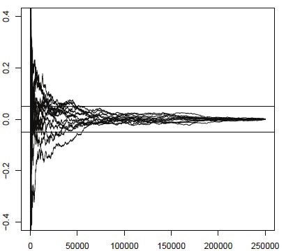
This number of burn-in cycles turned out to be sufficient to achieve
convergence of the Metropolis and Hastings algorithm regarding to the CUSUM
statistics proposed by Yu and Mykland (Yu and Mykland 1994). The CUSUM
plot is presented in Figure 2. We can see that the cumulative sums for the final
cycles (from 150 000 draw) do not exceed the interval (–0.05, 0.05). Therefore, it
can be assumed that the number of cycles was sufficient to achieve the convergence
and the final sample can be treated as draws from the stationary distribution.
That is why in the next step the final cycles were used to determine marginal
a posteriori distributions of γ1,...,γs and δ1,...,δr and calculate basic characteristics of
the a posteriori distributions (expected value and standard deviation).
12Transmission of Fertility Pattern in Mother-Daughter Relation – Bayesian view...
Figure 2. The convergence of CUSUM statistics for the MH algorithm
BAYESIAN MODELS COMPARISON
In order to build the most probable model that would reflect the empirical data
and the initial knowledge in the best way, Bayesian methods provide us with a very
intuitive formal model comparison framework (Jeffreys 1961, Greene 2003). As we
introduce a probability measure on the model space, we can use the Bayes theorem
to build a posterior on it. Posterior probabilities are calculated for each analyzed
model according to the Bayes theorem:
p y | Mi p Mi
p Mi | y m , for i 1,..., m , (7)
¦ p y|Mj p Mj
j 1
where p(yMi) is the marginal data density in the i-th model (or simply: probability
of our data when model i is applied), and p(Mi) is the prior probability of model
13Beata Osiewalska
i (conviction about model’s accuracy). Then the posterior odds ratio of two compet-
itive models should be calculated as follows:
p M1 | y p y | M1 p M1 (8)
PO Bayes factor u prior odds ratio
p M0 | y p y| M0 p M0
The posterior odds ratio provides information on how many times more probable
the first model is than model 0. For example, when PO=8, then model 1 is 8 times
more probable than model 0. When the prior probability of model 1 is equal to the
prior probability of model 0 (equal prior chances of each model), the posterior odds
ratio simplifies to the Bayes factor (BF). Usually, the value of the BF is presented
on a logarithmic scale. When 0Transmission of Fertility Pattern in Mother-Daughter Relation – Bayesian view...
that this estimator has two major disadvantages: the first – it has no finite asymptotic
variance, and the second – in small samples it overestimates the marginal data den-
sity (Lenk 2009, Pajor and Osiewalski 2013). That is why using HME could some-
times yield misleading results. Therefore, especially when the model comparison
procedure does not point out clearly the differences between competing models, it is
advised to use the adjusted HME with Lenk’s correction (Lenk 2009). Nevertheless,
in this study the standard HME will be used. The differences obtained with HME for
the two competing models under consideration (ZIP and standard Poisson) was so
big that including Lenk’s correction should not change the conclusion. In turn, results
for selection of covariates were confirmed by later results given by the posterior
distribution (to obtain the posterior distribution, HME is not needed). Therefore, in
this study using the standard HME could be justified. However, in the next studies
we plan to introduce the adjusted HME estimator.
THE FORMATION OF REPRODUCTIVE BEHAVIORS AMONG
AUSTRIAN WOMEN
VARIABLES DESCRIPTION
To analyze intergenerational transmission of reproductive behavior, the following
demographic variables describing the mother’s fertility pattern were chosen: number
of respondent’s siblings and mother’s age at respondent’s birth. It should be noted that
instead of mother’s age at respondent’s birth, the more appropriate variable seems
to be mother’s age at first birth. Unfortunately, such information was not collected
in GGS in Austria. Other variables were introduced in order to determine the basic
daughter’s characteristics, which also may have an impact on the analyzed number
of children, but they are not main interest of this study (treated as control variables).
These are: age (in years), educational level (highest educational level completed),
type of settlement (urban or rural areas) and marital status (whether respondent was
ever married). It should be mentioned that education, type of settlement and marital
status are treated as fixed over time with the value as in the moment of interview.
These characteristics in some cases could be different at the time when children were
born. If the proper data are available, these changes could be introduced using the
methods of Event History Analyses (EHA). However EHA concentrates mainly on
the duration between selected events and not on the total number of those events.
That is why, if the main interest of the study is to analyze the total number of births
and not the duration between births, the ZIP model seems to be more convenient.
To introduce the proper values of characteristics at the moment of birth of a child
(when known), other covariates could be included to the ZIP model as well (e.g., the
educational level at birth of a particular child). In some cases however, we should
expect that the correlation between included covariates (e.g., education at birth of
15Beata Osiewalska
the first child and education at birth of the second child) will be probably very
high. It could happen with covariates that generally do not change very often during
lifetime (like education, being ever married, etc.). That is why the current values of
characteristics such as education, marital status (treated as being ever married) or
type of settlement, could be treated as an approximation of those values during the
past life from a certain adult age, in case of lack of precise data.
Table 1 shows the structure of the sample population regarding the selected main
and control variables.
The variables number of siblings and mother’s age at respondent’s birth, describe
the fertility pattern developed in respondent’s family home. From the data structure
(Table 1), we can see that among the population of mothers, the typical number of
children was two (so one sibling), while the largest number of children reached 14
(13 siblings). The most common age at respondent’s birth was 23. The youngest
mother at respondent’s birth was 13 years old (3 women), and the oldest one – 46
years old (1 woman).
The first control variable type of settlement is divided into the following two
levels: urban and rural areas. The possible differences within life styles in these two
areas could influence the reproductive behaviors in a different manner. The majority
of respondents from the studied population lived in urban areas (59.4%).
Within education, the six following levels are distinguished: primary, lower
secondary, upper secondary, post-secondary, the first stage of tertiary, and the second
stage of tertiary education. These levels are subject to the ISCED7 classification
adopted in the Austrian educational system. The introduction of this variable is
justified by differences in reproductive behavior depending on education. The
majority of daughters have upper secondary education (50.1%), while primary and
second stage of tertiary education have only several respondents – respectively 15
women (0.5%) and 46 women (1.6%).
Marital status is divided into two levels, which split the population of women
into those who have never been married and those who are married or were at least
married once (so also widows and divorcees).
The population considered in this study (female respondents from the first wave
of Generations and Gender Study in Austria in 2008 and 2009) was born between
1963 and 1990, so at the time of survey these respondents were between 18 and
46 years old. In this group, there were only two 18-year-old women and only four
women who were 46. The number of respondents at the age from 19 to 45 was
similar in each particular age, with a slight predominance of older ages.
7
ISCED – International Standard Classification of Education designed by UNESCO
16Transmission of Fertility Pattern in Mother-Daughter Relation – Bayesian view...
Table 1. Data structure
Variable Level Structure
0 – rural 40.6%
Type of settlement
1 – urban 59.4%
1500
1 – primary 1250
2 – lower secondary 1000
Education 3 – upper secondary 750
500
(ISCED codes) 4 – post secondary 250
5 – 1st stage of tertiary 0
6 – 2nd stage of tertiary 1 2 3 4 5 6
0 – never married 46.0%
Marital status
1 – at least married once 54.0%
160
140
120
100
80
Age 60
40
20
0
18 20 22 24 26 28 30 32 34 36 38 40 42 44 46
1000
800
600
Number of siblings 400
200
0
0 1 2 3 4 5 6 7 8 9 10 11 12 13
250
200
150
Mother’s age at
100
respondent’s birth
50
0
13 15 17 19 21 23 25 27 29 31 33 35 37 39 41 43 45
17Beata Osiewalska
PRIOR MODEL ASSUMPTIONS AND POSTERIOR RESULTS
The need for a model that would allow analysis of a larger than expected number
of zeros was supported by a formal Bayesian models comparison. The ZIP model
was compared with the commonly used standard Poisson regression model. The
prior probability was the same for each model (0.5 for ZIP and 0.5 for standard
Poisson). The results clearly pointed that the ZIP model is much more adequate for
the analyzed data – the decimal logarithm of the posterior odds ratio (in that case
equal to the Bayes factor) is equal to 64. It means that the ZIP model is 1064 times
more probable than the standard Poisson regression.
The ZIP model is based on γ and δ parameters (with dimensions s=r=7) for which
the following a priori distributions were chosen:
J ~ MVN 0 >7 x1@ , diag 1, 1, 1,0.0 1, 1, 0.01, 1 (11)
G ~ MVN 0 >7 x1@ , diag 0.05, 0.05, 0.05, 0.0005, 0.05, 0.0005, 0.05 (12)
The hyperparameters of the a priori distributions were chosen to both enable all
possible values and remain coherent with the common knowledge in the case of a
hypothetical woman. It has to be emphasized that in fertility analyses of contemporary
populations, the prior distribution should set higher probabilities for smaller numbers
of children (from zero to 3) and at the same time very low probabilities (even equal
zero) for numbers of children bigger than 15.
Let x be a covariate vector representing features of a chosen respondent, for
example, x = (0, 4, 1, 30, 2, 23, 1) represents a woman who lives in rural area, has
post-secondary education, is married, is 30 years old, has 2 siblings and her mother
was 23 at the respondent’s birth (1 on the last place stands for the intercept). Then,
based on 10 000 draws from priors of γ and δ parameters, p and λ distributions for
the chosen respondent were determined (Figure 3).
Subsequently, we specified the a priori distribution of number of children for the
chosen woman (assuming prior distributions as previously). Results are presented
in Figure 4. As we can see, the distribution of number of children assigns non-zero
probability for all expected a priori values, therefore it seems to be a reasonable
expression of our initial knowledge about the analyzed variable before looking into
the data.
18Transmission of Fertility Pattern in Mother-Daughter Relation – Bayesian view...
Figure 3. The p and λ distributions for a chosen woman
Figure 4. The prior distribution of number of children for a chosen woman
1.0
0.8
0.6
0.4
0.2
0.0
0 1 2 3 4 5 6 7 8 9
To build the final model, which has the most adequate set of covariates,
and to check if there are some competitive models, Bayesian comparison was
applied. Each time two models were compared: a full model (with all covariates)
and a model without one chosen covariate. The prior chances for these models
were always equal. When a covariate occurred to be negligible then the new “full
model” is created (a model without this covariate) and the comparison starts again.
The procedure is finished when there are no other negligible covariates. The decimal
logarithms of the Bayes factor for the full model versus the model without one
covariate are presented in the Table 2. The BF for the covariate number of siblings is
equal 7.1. It means that the full model is a posteriori 107.1 times more probable than
the model without the number of siblings. The similar result is visible for mother’s
19Beata Osiewalska
age at respondent’s birth (BF equals 2.8). The smallest value of BF occurred for the
control covariate type of settlement, but still the value 1.0 means that full model is
better than model without this covariate. The analysis confirmed that the a posteriori
most probable model is the model with all chosen covariates. There is no need for
the Bayesian pooling approach8.
Table 2. Logarithms of the Bayes factors
Logarithms of the Bayes factor
Variable
(full model vs model without the covariate)
Type of settlement 1.008
Education 14.090
Marital status 118.835
Age 68.119
Number of siblings 7.069
Mother’s age at respondent’s birth 2.800
Marginal a posteriori distributions of all considered parameters are shown in
Figures 5 and 6. The dotted line represents the corresponding prior in order to
compare the two distributions and illustrate the strength of inference about the
selected parameter based on the data. In turn, the dots mark 2.5% and 97.5%
quantiles, which are helpful in determining the impact of the parameter on the
modeled variable number of children ever born. If a zero value in the marginal
a posteriori distribution of the parameter lies outside the interval set by the quantiles
(so-called the highest posterior density interval – HPD), then it can be assumed
that it has a significant impact on the analyzed phenomenon. However, if there is a
substantial probability that the parameter can be equal zero (so zero belongs to the
HPD interval) then its effect is treated as neutral or negligible.
It should be noted, that all obtained marginal posterior distributions compared
to corresponding priors are more centralized around its expected value, otherwise
the dispersion of these distributions is substantially lower. This fact leads to the
conclusion that the inference about parameters is strong.
8 To check formally that there is no need for knowledge pooling, the distributions from full model
and model with the lowest BF (model without type of settlement) were combined. The full model was
taken with the weight equal to 10BF/(10BF+1)≈0.91; the second model had weight 0.09. The results given
by pooled model were compared to the results obtained from the full model. There was no relevant
differences.
20Transmission of Fertility Pattern in Mother-Daughter Relation – Bayesian view...
Figure 5. The marginal posterior distributions – the zero model
J1 J2
J3 J4
J5 J6
J7
21Beata Osiewalska
Figure 6. The marginal posterior distributions – the count model
G1 G2
G3 G4
G5 G6
G7
22Transmission of Fertility Pattern in Mother-Daughter Relation – Bayesian view...
The (pseudo) random sample obtained from the a posteriori distribution (final
cycles) was used to determine the basic characteristics of the marginal distributions,
such as the a posteriori expected value and a posteriori standard deviation. The
results, presented in Table 3, are coherent with results obtained from the Bayesian
model comparison: the type of settlement seems to be the least important in the
analysis, while the strongest impact was marital status.
Table 3. The posterior expected values and standard deviations
Zero model Count model – Poisson
Variable Parameter E(γY) d(γY) Parameter E(δY) d(δY)
Type of settlement γ1 0.268 0.138 δ1 –0.095 0.053
Education γ2 0.436 0.073 δ2 –0.073 0.029
Marital status γ3 –2.441 0.147 δ3 0.403 0.080
Age γ4 –0.123 0.010 δ4 0.024 0.004
Number of mother’s children γ5 –0.177 0.046 δ5 0.045 0.015
Mother’s age at respondent’s
γ6 0.039 0.012 δ6 –0.010 0.005
birth
Intercept γ7 2.254 0.427 δ7 –0.317 0.179
In case when zero belonged to HPD interval (between 2.5% and 97.5% quantiles) the value was
marked with grey.
DAUGHTERS’ FERTILITY ACCORDING TO CHOSEN CHARACTERISTICS
To specify the impact of selected covariates on the a posteriori expected number
of children let us choose, as an example, one respondent by setting the value of j,
j=1,…,n (in the studied data set n = 2896). For this purpose, let the respondent be
a typical woman in the analyzed sample with the following characteristics: a woman
living in the urban area with upper secondary education, who is or was married, has
one sibling and her mother was 23 at the respondent’s birth. Let x be a covariate
vector representing features of this respondent, so x = (1, 3, 1, age, 1, 23,1). The
age of the woman will be set as 25 and 45 to allow the comparison of a young
woman who could just set the family and a woman who is almost at the end of her
reproductive age.
Let’s have a look at covariates representing fertility patterns developed in the
origin- family home. The first covariate, number of siblings, showed an important
effect on a woman’s procreative behavior. The a posteriori expected value of the
23Beata Osiewalska
parameter γ5 is negative (–0.177) and positive for δ5 (0.045). Therefore, we could
say that the more siblings a woman has, the bigger family she will set. The posterior
probabilities of a particular number of children due to the different numbers of
siblings are shown in Figure 7. To make the figure more clear, only three different
numbers of siblings (0, 2 and 4 siblings) and only numbers of children less than or
equal to 3 are presented. The upper plot is for a 25-year-old woman, while the lower
one is for a woman who is 45. Both plots are for a typical woman – all covariates
are set except for the number of siblings: x = (1, 3, 1, 25/45, number of siblings,
23,1). In this, as in other figures of this type (so-called box-whiskers plot, Figures
7 and 8), a thick black line is the posterior median, rectangular boxes represent the
interval set by the first and third quartile (25% and 75%), and whiskers cover the
2.5% and 97.5% quantile interval. The highest posterior probability for a 45-year-
old woman who has siblings is for two children, while a woman who grew up as an
only child would probably have one child. Additionally, it could be said that women
with siblings decide to have a child at a younger age than women with no siblings:
a 25-year-old woman is less probable to be still childlessness when she has siblings
than when she is an only child.
The second fertility pattern covariate, mother’s age at respondent’s birth also
significantly determines the number of a woman’s children. Posterior probabilities
for number of children due to mother’s age at respondent’s birth are presented in
Figure 8. We can see that the older the mother was at the respondent’s birth, the
lower posterior probability that the daughter will have many children. A 25-year-
old woman, whose mother was 45 at her birth, would probably be childless, while
a woman of the same age whose mother was young (18 years old) at the woman’s
birth would already have one child. Finally, for a woman of age 45, the most
probable number of children if her mother was 18 at her birth is two children, and
if her mother was older at her birth, one child.
To summarize, the impact of both covariates number of siblings and mother’s age
at respondent’s birth on the daughter’s number of children ever born, reveal that her
mother’s fertility pattern affects a woman’s procreative behavior.
Selected control variables generally appeared to be important for women’s
family models. The first control covariate – type of settlement has a slight impact on
childlessness, but simultaneously no impact on parenthood was revealed. Education
of a woman has a significant influence on both childlessness and parenthood: the
more educated a woman is, the higher posterior probability of her childlessness and
lower probability of having many children. The next covariate is marital status,
which turned out to be very important in the analyzed population, its impact on
number of children ever born is the strongest among all other covariates. Therefore,
it could be said that marital status in Austria still strongly determines procreative
behaviors.
24Transmission of Fertility Pattern in Mother-Daughter Relation – Bayesian view...
Figure 7. The posterior probabilities of particular number of children for a different number of
siblings
0.5
0.4
0 sibl
2 sibl
4 sibl
0.3
0.2
0.1
0.0
0 1 2 3
0.5
0.4
0 sibl
2 sibl
4 sibl
0.3
0.2
0.1
0.0
0 1 2 3
Upper plot – 25 years old woman
Lower plot – 45 years old woman
25Beata Osiewalska
Figure 8. The posterior probabilities of particular number of children for a different mother’s age
at respondent’s birth
0.6
0.5
0.4
18
30
0.3
45
0.2
0.1
0.0
0 1 2 3
0.6
0.5
0.4
18
30
0.3
45
0.2
0.1
0.0
0 1 2 3
Upper plot – 25 years old woman
Lower plot – 45 years old woman
Parameters γ7 and δ7 represent intercepts in the zero and count model. The first
one – γ7 determines the “basic” value of probability of childlessness in case the other
covariates in the analysis occur to be unimportant. Its a posteriori expected value
is 2.254, thus the “basic” expected probability of zero equals 0.905. The second
one – δ7, which specifies the “basic” average number of children, turned out to be
insignificant.
26Transmission of Fertility Pattern in Mother-Daughter Relation – Bayesian view...
PROCREATIVE BEHAVIORS BY FEMALE PROFILES
In the previous section it was demonstrated that procreative behaviors are different
due to social and demographic characteristics, such as age, educational level and
marital status. What is more, this study revealed that the reproductive behaviors
also depend on fertility patterns developed in the origin-family home. Therefore,
determining women’s procreative behaviors due to different female profiles seems
to be valuable for such analyses.
To analyze the a posteriori distributions of the number of children for the
chosen females’ profiles, the Bayesian approach was crucial. Inference about these
distributions would be impossible within the classical approach – we would not
be able to obtain full knowledge about the distributions of nonlinear functions of
parameters, such as the probability of childlessness or expected number of children.
In this study we defined five types of women. The first two profiles presented
below are defined in order to demonstrate procreative behaviors of 35-year-old
women with different family background:
A – siblings profile for typical women with different number of siblings:
xA = (1, 3, 1, 35, siblings, 23, 1);
B – mother’s age profile for typical women with different age of mother at their
birth: xB = (1, 3, 1, 35, 1, age, 1).
The next three profiles are connected with social and demographic conditions
and are presented for 25, 35 and 45-year-old women:
C – typical woman with the following characteristics (which occurred most often
in studied dataset): living in urban area, with upper secondary education,
married, has one brother or sister and her mother was 23 at the woman’s birth,
xC = (1, 3, 1, age, 1, 23, 1);
D – single educated woman, so a respondent with characteristics as follows:
living in urban area, with second stage of tertiary education, she has never
been married, has no siblings and her mother was 28 at the woman’s birth,
xD = (1, 6, 0, age, 0, 28, 1);
E – married educated woman – a respondent with characteristics like single edu-
cated woman, but married, xE = (1, 6, 1, age, 0, 28, 1).
The differences in fertility patterns of types C and E are mainly due to the level
of education, while types D and E are chosen to emphasize the strong impact of
marital status on the a posteriori expected number of children.
The posterior distributions of expected number of children for A and B female
profiles are presented in Figure 9. The differences between women with other family
background are visible and important. The posterior distribution of expected number
of children due to number of siblings is presented in the upper plot in Figure 9. The
following conclusion could be made: when a woman grew up in a big family, with
many siblings, it is much more probable that she will follow the same pattern in
27Beata Osiewalska
her own family and decide to have more children, than a woman who grew up as
an only child. A 35-year-old typical woman with 4 siblings would probably have
2 children (the a posteriori expected value is 2.014), while among women with no
siblings one in three would have only one child (the a posteriori expected value
is 1.699).
Additionally, mother’s age at respondent’s birth seems to have an important
influence on a woman’s procreative behaviors. The posterior distribution of expected
number of children is presented in the lower plot in Figure 9. We can see that when
a mother gave birth to a daughter at an older age, then the daughter will probably
have fewer children. The a posteriori expected number of children for a 35-year-
old typical woman, whose mother was 18 at her birth, is 1.783, and 1.316 for those
whose mother was 45. This connection between daughters and mothers could be
explained as follows: daughters compare their procreative behaviors with fertility
patterns from their origin-family home, so when a mother gave birth to a daughter
at her young age, then the daughter would earlier set her own family, so it is more
probable that she will have more children.
Then, according to the next three profiles, the posterior distributions of the
expected number of children are shown in Figure 10. Let’s start from type C. The a
posteriori expected number of children for a 25-year-old typical woman is equal to
1.261. In other words, among 25-year-old typical women, approximately one in four
women have two children, while the other three have one child. For older women the
proportion is changing. For a 35-year-old typical woman, the a posteriori expected
number of children is equal to 1.777, and for a 45-year-old woman it reaches 2.228.
It can be explained as follows: among 35-year-old women of type C, 75% already
have two children, and 25% have one child. Finally, among the 45-year-old female
population, three in four typical women have two children, and the other one in four
have three children.
The next type is single educated women with the following characteristics: never
married, fully educated woman who lives in an urban area. The posterior distribution
of the expected number of children is presented in the middle plot in Figure 10. It can
be said that almost for sure a young woman of type D would not have any children,
since the a posteriori expected number of children is 0.057 and the distribution is
strongly concentrated around its mean. For older women the deviations are bigger,
but distributions are still strongly separated from 1. The posterior expected number
of children for a 35-year-old single educated woman equals 0.189 and for a 45-year-
old, 0.535. Thus, it can be said that 50% of 45-year-old women with D characteristics
would have one child, while the other half would stay childless. Having more than
one child is hardly probable here.
28Transmission of Fertility Pattern in Mother-Daughter Relation – Bayesian view...
Figure 9. The posterior distributions of expected number of children for type A and B
Upper plot – type A
Lower plot – type B
Finally, the posterior distribution of the expected number of children for married
educated woman is presented in the lowest plot in Figure 10. These distributions
compared with previous distributions for the D type (middle plot) show the strength
of marital status. We can see that half of 25-year-old woman with E characteristics
would already have one child (the a posteriori expected value is 0.509). A 35-year-
old married educated woman would probably have one child, while among 45-year-
old women, two in three would already have two children.
29Beata Osiewalska
Figure 10. The posterior distributions of expected number of children for type C, D and E
7
6
25
35
5
45
4
3
2
1
0
0.0 0.5 1.0 1.5 2.0 2.5 3.0
30
25
25
35
20
45
15
10
5
0
0.0 0.5 1.0 1.5 2.0 2.5 3.0
7
6
25
35
5
45
4
3
2
1
0
0.0 0.5 1.0 1.5 2.0 2.5 3.0
Upper plot – type C
Middle plot – type D
Lower plot – type E
30Transmission of Fertility Pattern in Mother-Daughter Relation – Bayesian view...
CONCLUSIONS
Based on the results of the research, general conclusions about the methodological
and cognitive side of the study might be formulated. With regard to the method of
analysis, it should be noted that the Zero-Inflated Poisson model and Bayesian
inference form a useful framework for analyzing transmission of fertility patterns
developed in the origin-family home. Within this study, the model allowed us to
investigate the effect of fertility patterns developed in the origin-family home, as
well as other selected demographic and social variables, separately on childlessness
and parenthood in the population of daughters. Generally in fertility analyses, the
Zero-Inflated Poisson model seems to be particularly useful when the special research
interests are given to the total number of children (actual or intended), because
the ZIP model gives a different qualitative dimension (value) to childlessness and
parenthood. Within the ZIP model it is possible to analyze one set of covariates that
could determine childlessness and another for parenthood (e.g., we can expect that
enlarging family is influenced by the costs of rearing the previous children, while for
childlessness these costs do not even exist). Simultaneously, we still keep these two
states, which could be determined by different characteristics, under the one fertility
model – so possible dependencies between those states (one state is connected to the
other by the probability of childlessness/parenthood) are allowed.
In turn, the Bayesian approach enabled us to estimate the posterior distributions
of having a certain number of children depending on the fertility pattern developed
in origin-family home and other socio-demographic characteristics of a woman
(distributions of expected number of children by female profiles). The uncertainty
of the results are rather low, and the variances of the posterior distributions
are small, so we are able to point out the differences clearly and the results are very
precise.
Both components of the model (zero and count) were based on the same set of
variables that characterize the mother’s fertility pattern (number of children and
age at respondent’s birth) and social and demographic characteristics of daughters
were included as control variables (age, type of settlement, education and marital
status).
This methodological approach applied to GGS data for Austria have revealed
that family procreative behaviors among contemporary populations are affected by
the fertility pattern of the previous generation. Regarding the number of siblings,
the results occurred to be coherent with the previous studies: there is observed the
positive correlation between a mother’s and a daughter’s family size. Additionally, it
was found that mother’s age at daughter’s birth is important for a daughter’s number
of children. The mechanism of the mother-daughter fertility pattern transmission
could be explained as follow. Women compare her own family model with the
pattern developed in the origin-family home. The origin-family pattern is likely to
be treated as proper or safe (because it is known) and that is why it is likely to be
31You can also read