Tuning loop: control performance and diagnostics
←
→
Page content transcription
If your browser does not render page correctly, please read the page content below
Tuning loop: control performance and diagnostics

                   Nunzio Bonavita, Jaime Caserza Bovero, Riccardo Martini
                             ABB Process Solutions & Services SpA
                                 Via Hermada, 6 – 16154 Genoa

                                             Summary
This article intends presenting an innovative solution for controlling the performance of tuning
loops. The software product has been designed to enable process managers to recover profit margins
through the systematic monitoring and adjustment of the performance of the basic control system. To
achieve this aim, technologies and methods are systematically used that have been developed in
research and development laboratories on the basis of the results produced over the past 15 years in
the fields of control engineering and information technology.

Keywords: Control performance monitoring, loop tuning optimization, model identification

1 INTRODUCTION
Ever since the early 90s, there has been a renewed and careful interest in the evaluation of basic
control loop performance. This has been caused by the contemporaneous existence of two
stimulation factors, one academic and the other economic/managerial.

On the one hand, the work of Harris [1], has re-launched a field of research that had seemed to be
gradually losing ground, presenting a simple and effective method for the objective evaluation of
tuning loop performance, with a measurement that can be compared with the determination of the
“state of form” of the loop. At the same time, there has been increasing attention in the field of
continuous processes towards the careful management of basic control systems. In other words, there
has been a growing awareness of the impact these have on production processes, both directly and as
a binding condition for the effectiveness and relevant economic return of more sophisticated
automation strategies.

The growing demand has naturally been intercepted by industrial automation suppliers who continue
to be engaged in developing and marketing products and solutions for monitoring tuning loop
performances.
The successful application of these products depends on a series of factors that go beyond the pure
effectiveness of the calculation algorithms of the various loop performances, including the ability to
connect up without disturbing the system forming the subject of the evaluation, easy use and
configuration and the possibility of translating the inevitably obscure figures into a concise number
of precise data useful for the control room operator or maintenance engineer.
Nevertheless, even a punctual and accurate diagnostic capacity is often not enough. The drastic
reduction of the workforce on production sites does in fact force the professional figures in charge of
operations to take on several diverse duties and consequently the need arises not only to identify the
nature of the problem but to also be able to solve it with quick, safe and easily implemented remedial
measures.

This work intends presenting a number of solutions recently placed at disposal by the market in the
form of a product that combines monitoring and diagnostic functionality with instruments for
effectively intervening on the control system in order to restore it to optimal operating conditions.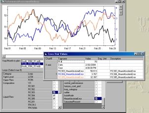
The article is organised as follows: after a short historical digression on the basic principles of
control system performance monitoring, section 2 focuses on the requirements, the restraints and the
opportunities which the application of these techniques offers in the field of process automation.
Section 3 is dedicated to the description of the salient aspects of the proposed solution, while section
4 supplements the treatise with a short example of application. Finally, section 5 is dedicated to
future prospects and scheduled improvements.

2    EVALUATION OF CONTROL SYSTEM PERFORMANCES: STATE OF THE ART

The availability1 and effectiveness of a control system is clearly important for managing the process
in conditions of safety and maximum performance, ensuring quality of production and its
profitability.
Over 90% of the process control systems are based on PID type controllers, which represent a basic
standard2 as regards process tuning.

                                                    Control Output                                 Variable
                 Setpoint         Error    Regulator
                                             PID                 Actuator           Process
                            -
                                 Process variable

                                                               Sensor

                                          Figure 1 - Tuning loop with PID diagram

These controllers, the basic principle of which is fairly simple, represent the basis of any automation
strategy, including in the case of second level systems, such as multivariable controllers or MES
(Manufacturing Execution Systems).
The most general expression of the algorithm of the PID controller consists in the so-called "parallel"
expression, in which the three proportional, integral and derivative parts operate in a non-interacting
way on the feedback error. Including the possibility of a weight factor on the proportional part and of
a derivative action on the process variable or on the error, this can be written as follows:

                                u = K P (β ⋅ r − y ) + K I     (r − y ) + K D s (γ ⋅ r − y )
                                                             1
                                                             s               1 + TF s
where:
         u        Manipulated Variable (Controller action)
         r        Setpoint
         y        Process Variable (Controlled Variable)
         KP       Proportional Gain
         KI       Integral Gain
         KD       Derivative Gain
         TF       Time constant (Filter)

1
  By the word availability is meant in this case the relation between the time the loop is able to operate in closed chain
with appropriate performances compared to the total operating time, including therefore the open chain operating time.
2
  Notice that, though the PID concept is fairly widespread, its practical implementation in the various control and
automation systems is very varied, presenting different variations.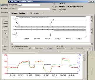
β        Setpoint weight factor in proportional part 3
         γ        Setpoint weight factor in derivative part 4

The parameters KP, KI e KD represent the "knobs" at the disposal of the control engineer which
permit combining the characteristics of the controller with the actual dynamics of the process to be
governed, so as to obtain the required answers and behaviours. We thus found ourselves faced with a
system with 3 distinct degrees of liberty for which the best value threesome must be pinpointed.
Because the overall process performances will depend on the goodness of the tuning done, it follows
that this appears as the crucial step in commissioning a plant. For this reason, it is normally entrusted
to specialists who enter the optimal values of the three parameters on the basis of empirical rules or
principles based on personal and therefore not easily transferable experience.

With the passing of time however, changes in production conditions or normal settling of component
parts, sensors and actuators can affect the effectiveness of regulation. These changes can vary from
changes in process gain or dynamics, to valve operation problems (stiction5, hysterisis) to the
application of restraints on operating conditions. The moving away from original tuning conditions
would therefore call for the periodical retuning of the controllers, so as to adapt tuning to changes in
operating conditions6.
Monitoring and restoring the operation of the entirety of plant controllers is however a pretty onerous
business as regards personnel commitment. More specifically, such requirement clashes both with
the considerable reduction in staff under way for some time now in all production sites, and with the
scarcity of people truly expert in the field of control system tuning. The lower availability of time
and resources inevitably leads to neglecting major aspects of process management which
nevertheless have an impact on the global economical bill. Part of this category are the maintenance
requirements of regulating instruments and parts. Persistent temperature fluctuations caused by a
valve in hysterisis or a badly tuned controller will have to be offset by the continuous use of hot
and/or cold fluids, the cost of which will accumulate in an insidious but not negligible way on the
energy bill and consequently on variable production costs [2].
A further contribution to the drop in economic performance also comes from the objective difficulty
of tuning procedures. A very high percentage of industrial controllers does in fact lack the derivative
part by need rather than by choice. In practice, the decision is made not to use a PID controller not on
the basis of a comparative analysis of performances (which at least in the case of processes
distinguished by second order or superior dynamics, would be far better) but due to the extreme
difficulty of manually tuning a system with three independent parameters [3]. In other words, the
lack of mathematical supporting instruments translates into the resigned acceptance of lower
performances.

In practice, we are faced with a situation distinguished by [4]:
            • from hundreds to thousands of loops
            • system complexities (both process and automation)
            • multiple and sometimes contrasting control goals
            • long maintenance cycles
            • low availability of operating and engineering personnel
            • severe economic impact

3
  For β=0 the proportional part acts on the PV while for β=1 it acts on the deviation
4
  For γ=0 the derivative parts acts on the PV, while for γ=1 it acts on the deviation.
5
  The English term Stiction identifies all those events due to friction on the valves
6
  It should be noted that this type of problem can in some cases can be completely inherent in the specific type of
  production and not relate to the history of the unit and equipment. This is the case of plants working with campaign
  productions (frequent in fine chemistry) where the load conditions and the type of product can be greatly different from
  one period to another, leading to the need for personalised tuning for the different production campaigns.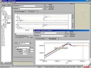
The existence must be emphasised of a perception problem on the part of the management, ready to
acknowledge the positive economic impact of cutting back the number of staff, but less inclined to
accept the actual drop in margins caused by failure to maintain the process at potential efficiency
levels. This leads the company management to focus on production efficiency increases tied to cuts
in the number of staff, while underestimating the benefits produced by better management of
company assets.
Hence the need to have instruments and methods able to keep a check on the performance of
controllers, warning and requesting human assistance only when actually required [5].
To cater for this need, in the past 15 years, strong research and development efforts have made it
possible to develop a series of methods for monitoring control loop performances essentially based
on the evaluation of variance in the controlled variable in the face of stochastic disturbances than
cannot be measured ([6], [7]).
Most of these methods are based on the work of Harris [1], who suggested using the closed-loop
collected data to assess controller performances using the so-called minimum variance control
(MVC) as an objective benchmark.
Without going into technical details, which do not fall within the scope of this work (for more details
see, among others, the excellent survey provided by [8]), it will be enough to recall that, from a
theoretic viewpoint, a minimum variance controller is a controller able to remove all disturbance
effects (downstream of the delay time), leaving only a disturbance of the white noise type. Given any
disturbance frequency, no controller can do a better job in reducing the variance of controlled
variables and, in other words, an MVC controller represents the best theoretical result that can be
achieved.
It is its very nature as "asymptotic maximum" that makes it an ideal benchmark for the construction
of an objective measurement of the performances of a controller.

Harris' index is nothing more than the relation between the MVC control loop variance and the
variance actually measured:

                                                   σ MVC
                                                     2
                                              I=
                                                   σ SP
                                                     2
                                                        − PV

Harris' index is therefore a number between 0 and 1: the higher the number, the higher the controller
performance to the theoretical maximum. It belongs to stochastic [8] estimation methods, known by
this name because they evaulate the response of the controllers on the basis of their statistical
behaviour in the case of non-measured disturbances. It is not therefore able to provide any
information on the determinist performances such as the response to a step variation in the set-point
or disturbance, adjustment time, over-elongation, stability margin, etc.
Among its advantages must be mentioned its capacity to build an objective principle of evaluation of
performances, its uniqueness (the σ2MVC value is independent of the controller structure) and its
relative ease of calculation in standard industrial computers. Harris' index best expresses its potential
(and is directly applicable) in the following cases:
    • processes without major delay times (for instance in the case of carrying loops);
    • processes describable with low-order models;
    • processes where non-measurable disturbances are almost stationary

It is however necessary to recall that this is not applicable to processes with variable delay times and
that an adequate compromise must be assessed from time to time between the stochastic
performances and the determinist performances. To this end, it is therefore necessary that the
judgment on the performances of a control loop be suitably mediated on a series of different
evaluation parameters [9].
3 AN INNOVATIVE SOLUTION FOR THE INTEGRATED MANAGEMENT OF
CONTROL LOOPS
In section 2 we saw how the gradual reduction of plant personnel forces the remaining technicians to
take on a growing number of tasks and duties. This results in less and less time and energy being
available for dedicating to monitoring process performances. To try and quantify the efforts required,
we should consider that, in typical industrial situations, a control engineer has to maintain on average
4-500 loops at top performance. Considering that the analysis and tuning of a controller requires not
less than 2-3 hours, it follows that keeping a control system in shape takes up between 6 and 9
months work of a highly qualified technician.
Luckily, the widespread availability of computers and of large quantities of data in real time permits
automating tasks that until a few years ago would have been unachievable without extensive human
intervention.
Figure 2 - Typical automatic multi-level structure
It is on the backdrop of this scenario that the authors of this memo have been engaged for some years
in designing and developing new products for the application of the most recent information
technology solutions in the field of automation. Such development programme, which has already
produced innovative software instruments for advanced process control [10], has recently been
enhanced with a solution for the optimisation and maintenance of basic tuning management.
The product, called OptimizeIT Loop Performance Manager (LPM) consists of a system for the
systematic evaluation of the state of health of control loops (forthwith identified as loop auditing)
and of a system for the assisted tuning of the loops themselves (loop tuning).
Figure 2 shows the role played by a package such as LPM in the traditional automation architecture
for continuous processes. The crucial stages in the application of such a product will be briefly
illustrated below.
3.1 Installation and configuration
The main raison d'etre of a product like LPM is to reduce the work load for the plant personnel. In
view of this, a crucial requirement is the absolute ease of connection to the DCS and immediate use.LPM can connect up to any control system by OPC7 connection. Special wizards permit automatic
search for the OPC Servers on the net and their guided configuration. LPM is able to connect up to a
plurality of servers so as to centralise on a single platform the maintenance operations on several
DCS units, including of different suppliers: a special library does in fact permit interacting with the
numerous implementative variants of the PID algorithms available on the market.
To divide out the loops in an orderly way, these are grouped together and displayable according to
the areas of operation to which they belong: for instance, in a refinery, it will be possible to classify
the loops according to units to which they belong (crude unit, FCC, hydrocracker, utility, etc.).
The configuration of each single loop, a potentially onerous task in terms of time, tedious and most
definitely prone to the introduction of trivial entering mistakes, is assisted by a Bulk Configuration
utility able to import all the parameters needed from a derived Excel file, for instance, from the
database of the control system itself.
LPM Client
Tuning Auditing
LPM Relational
Database
Automation System
LPM Server Connection
OPC or Direct
connection
DCS/PLC
System
Figure 3 – LPM architecture
Special attention has been given to making the instrument intuitive and easy to use by the control
room engineers. The only user interface, structured according to the most modern Microsoft
Windows® standards, does in fact permit accessing both the auditing routines and a sophisticated
environment for tuning the basic controllers, which have been pinpointed as susceptible to upgrading
by auditing. Figure 3 shows a simplified diagram of the LPM software architecture.
3.2 Auditing
The fundamental requirements of an automatic performance evaluation system are:
1. Safety: ability to interact with the control system in an absolutely safe and non-invasive way;
2. Autonomy: ability to control the various stages (data collection and processing, evaluation
production) in a fully automatic way;
3. Availability: the processed data must be stored and made available to the user at request,
even after time;
4. Interactivity: possibility for the user to perform monitoring operations at command
immediately whenever the need arises.
7
The product is also able to connect up directly, through high-performance proprietor protocols, to some specific DCS.LPM has been designed so that it is able to cater for this need through the following completely
automated procedures:
• Collection of periodical data for the loops subject to evaluation (data “batches”)
• Calculation of performance indices
• Filing of indices
• Performance of tests on indices to elaborate process diagnostics
AUTOMATIC DATA
CONFIGURATION
COLLECTION
• # Collection per day
• For each loop of every
• Specific parameters
defined category
per category
ON-LINE EVALUATION
• Performance index
trends
MAINTENANCE JOBS ON
SENSORS/ACTUATORS
REPORTING
• Diagnosis
• Loop Ranking Reports
• Custom Reports
NOT
OK
OK LOOP TUNING
SAVE/FILE
RESULTS
Figure 4 – Loop Auditing Flowchart
A system for evaluating tuning loop performances that intends using quality KPI such as the
previously described Harris index must be able to provide a reliable value of σ value which a
minimum variance controller would obtain on the single controller being examined.
This can be calculated through the use of a self-regressive model of the type shown in the following
expression:
ŷ(i + b ) = a 0 + a 1 y(i ) + a 2 y(i − 1) + a 3 y(i − 2) + .... + a m y(i − m + 1)
As we can see, for each controller, the user should provide a series of parameters such as the number
of terms to be considered in the model (m), the sampling interval, the extension of the data as a
whole (n) and the prediction horizon (b). It is of course evident that specifying these detailed
parameters for hundreds of loops would make the application of these methods impossible from a
practical viewpoint [11]. The large-scale application of assessment performance methods is therefore
tied to the ability to determine default values sufficiently generic for broad classes of controllers.
LPM permits grouping the controllers into categories (temperature loop, pressure loop, composition
loop, etc.) each of which can be distinguished by acquisition parameters (sampling frequency,
number and length of single batches, etc.) as best thought fit. According to the date configured by the
user, the programme will perform the required number of data collections at set times, operating in
background on several hundred loops per server. Some categories are left free (the so-called “User-defined Categories”) to permit controlling any loops which badly adapt to the default values of the
major categories.
After completing data collection, the program calculates a group of 41 different performance indices
and stores these in the auditing database. Of these, 3 are calculated in continuous mode (with
sampling every minute for all loop types) as a statistic reference (% of time in auto mode, % of time
in saturation, absolute mean error), while the remaining 38 are processed in batches, meaning at the
end of each collection operation and contain all the most significant details.
Although part of the 41 indices are not directly referable to diagnostic aspects, but represent material
useful for any detailed tests (for instance boolean status indices or high statistic moments), some
have to be intuitively interpreted by the control room and/or maintenance staff. This is not the place
to go into detail. Suffice it to say that some of the most important are:
• Harris index;
• Setpoint "Crossover" Index;
• Oscillation Indices. These include evaluations relating to the amplitude, the period and
severity of the oscillation, where this is defined as the relation between the variance due to
the oscillation and the overall variance of the signal.
• Operating Mode Index (auto/manual), expressed as % of the samples for which the loop was
in automatic out of the total of the batch samples;
• Saturation index, expressed as % of the samples in saturation out of the total of the batch
samples.
The indices remain at the disposal of the user, who can check the special time trends (Figure 5)
The reporting function generates weekly and monthly report files in Microsoft Excel format, that can
be configured by the user. These contain information of a quantitative (the values of the calculated
indices) and qualitative nature. The latter relate to diagnostic hypotheses processed on the basis of
tests performed on the performance indices themselves. Examples of the provided diagnostic indices
are:
• Tuning too “bland”
• Oscillation loop
• Valve not sealed
• Too much noise
• Check saturation
• Overall loop evaluation.Figure 5 – Example of Trend on evaluation KPI
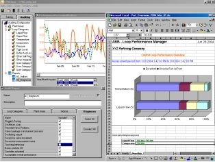
The user can also interact with the program at any time by configuring and asking for an additional
report which will be immediately produced. The reports enable the maintenance technicians to focus
on the major control problems and, when suitably stored, make possible plant performance
comparisons over the long period.
Figure 6 – Example of auditing and reporting
The auditing procedure placed at disposal by LPM is distinguished by a number of very interesting
characteristics:
• Calculation of numerous indices: literature often emphasises how the detection of faults and
malfunctions during control is only possible by the combined analysis of diverse indices [6];• Conversion into a small number of clear diagnostic suggestions, the values of numerous
indices often relating to statistic-operational aspects that are not uninteresting;
• Strengthening of the diagnostic results by explicit overall categorising of loops. Apart from
anything else, this permits defining a hierarchy among the loops requiring attention, on the
basis of their actual requirements;
• Continuity as regards monitoring on diverse time horizons. Entrusting to random samplings
can easily completely falsify the evaluation of the state of health of loops operating, for
instance, in very variable conditions.
3.3 Tuning
As Figure 4 shows, the auditing stage is able to detect problems or malfunctions relating both to
operation of the instruments or process components, and to their control by the automation system.
While in the former case, normal inspection and maintenance is essential, in the latter it is often
possible to obtain surprisingly successful results through the adequate tuning of the control loops.
For this purpose, to complete the "exploration" stage consisting of the auditing loop, LPM offers a
powerful and refined utility for the assisted tuning of base controllers.
• DATA COLLECTION • LOOP
• name the data set CONFIGURATION
• Connection to DCS • tagname
• Sampling time • Type of PID,
• Loop and Area,
• Definition of constants
and controller range
DATA SET
• IDENTIFICATION OF
MODEL
• Label the model
• Select the datasets,
• Select shape of
model, CHANGE
• Adjust filtering on • MODEL
noise EVALUATION NOT
• Comparison OK
MODEL
prediction-output
• Step response
• Bode Plot
TUNING
• Creating a tuning session OK
• Select tuning regulation
• FB Tune & Simulate
• FF Tune & Simulate • TUNING
EVALUATION CHANGE
• Simulation
TUNING • FB evaluation
NOT
PARAMETER • FF evaluation
OK
S
READY FOR DOWNLOADING
OK
Figure 7 - Loop Tuning Flowchart
The Loop Tuning procedure occurs in the following steps (Figure 7 - Loop Tuning Flowchart):
• Collection of process data through OPC linkup or direct linkup8
• Processing and storing of collected data
• Parametric identification of process models
• Evaluation of models obtained
• Calculation of values of the tuning parameters of the PID
8
Available for some automation systems• Evaluation of the performance of the controllers with new tunings through simulations
• Filing results and tuning procedures in special logs.
The first step of the tuning procedure consists in data collection. In this case data collection requires
an operator to prompt the process with a series of modest variations such as not to disturb normal
system operation. LPM permits collecting data both with open loop (meaning with the controller in
manual) and in closed loop (controller in automatic).
The robust identification algorithms at disposal permit identifying models of growing complexity
including those with reverse or over-dampened response. By selecting a specific flag, models can be
identified for integrator processes (level controls). The identification process occurs in separate
steps: the software first of all identifies the delay time subsequently used to determine the complete
transfer function. This approach adds flexibility to the system, allowing the user to manually enter
previously known parameters and leaving to the software the task of finding the missing or uncertain
ones. The models can be built from among:
a) Controller output and Process Variable to be used for feedback tuning;
b) Measured Disturbance and Process Variable to be used for feedforward tuning.
Great emphasis is given to the model adequacy evaluation phase: for this purpose, the user can
examine both the plot (prediction vs. real data, step response, frequency response) and numerical
merit factors (R2, mean quadratic error).
Once an adequate process model has been identified, this can be used for the real tuning phase. LPM
places at disposal the following tuning rules:
• lambda tuning;
• dominant pole placement for PI controllers;
• dominant pole placement for PID controllers;
• Internal Model Control for PI controllers;
• Internal Model Control for PID controllers.
In our opinion, the tuning rules at disposal offer a range of alternatives that successfully cover the
various possible occurrences related to continuous process systems. The choice of tuning method is
not affected by factors such as type of process model, control scenario and design criteria.
By way of example and without going into detail, we can say that generally speaking, the Internal
Model Control and Lambda tuning method are preferable when the major requirement is the capacity
to pursue set-point variations (e.g., in the master controller in a cascade configuration), while
dominating pole positioning is more successful as regards disturbance rejection.Figure 8 – Example of tuning performed with LPM
An optimisation algorithm calculates the best tuning parameters and presents simulations of the
controller response both to input disturbances and setpoint variations. Plot analysis is completed by
numerical indices such as the integral of absolute error, the overshoot value (9) or the settling time.
This way the user can select the type of tuning most effective for his purposes not only on the basis
of his experience or impressions deriving from a sight examination (necessarily subjective) of the
simulation graphs, but also comforted by objective numerical parameters.
Finally, the user can also perform a last “fine tuning” adjusting the parameters by means of
convenient sliders, that make it possible to comfortably explore the margins of uncertainty and
stability of the controllers and find the best compromise between sturdiness and response
performance.
Once the best tuning has been found for the feedback part, the user can use a similar procedure to
also tune the contribution of the feedforward part, on the basis of the identified models as described
in para. b) above.
Before closing the tuning activity, LPM saves the results of the session in special logs that go to form
a sort of historical archive of all the jobs done on the loop. The importance should be emphasised of
the “book-keeping” function as regards routine system operations. Storing over time details of the
criteria and procedures that have resulted in the past in certain tuning parameters being selected does
in fact permit protecting oneself against common risks deriving from staff turnover and eliminates
the natural hesitation of younger and less expert personnel to change whatever is "in any case
operating".
9
Overshoot is the term given to the difference between the
peak of the transitory response and the normal operating
value of a process output (PV), with respect to a change
made on the process input (CO).
A response with overshoot does not necessarily represent
an intolerable behaviour; on the contrary, especially if the
peak is short and not pronounced, it can be judged
according to the speed the setpoint proximity is reached
with this response.Finally, it must be added how a prominent feature of the products consists of the possibility of
performing tuning operations at the same time as normal monitoring functions.
Figure 9 – Example of Tuning Log
4 EXAMPLE OF APPLICATION
One of the most interesting aspects relating to this type of technology relates to the benefits and the
practical difficulties its use entails.
A first aspect to be considered is the complementarity between tuning and auditing, both in the phase
of maintenance of existing systems and in the phase of commissioning new applications.
Let us take for example the case of an adjustment loop re-tuning job relating to a polymer production
plant, in which the authors have taken part. In this case, the plant has been running for decades and
the field instruments, as regards both the sensors and the actuators (valves, pumps, etc.), are rather
old; loop tuning was first performed when the plant was started up and the relevant maintenance was
done in a non-systematic way, with the practical result that some loops are well tuned and updated
while others have tuning parameters dating back years and years.
In a case like this, one possible approach is to perform a blanket tuning of the entire loop, perhaps
split up into units. This way, by analysing the loops one by one, the functionality can be checked of
the field instruments and the tuning can be done. An activity of this kind would require, for the loop
screening activity only, hundreds of hours of work on the part of an expert technician.
An alternative procedure would on the other hand be to configure the auditing functions and acquire
data and information on the shape status of the various loops; this way it is easier to identify and
categorise the problems of the various loops, before the tuning activity; this permits anticipating the
solution to any problems and makes it possible, through the re-modulation of the activity plan, to
maximise overall efficiency. An example of the obtainable benefits will be appreciated by
considering maintenance of a valve affected by malfunctions, one of the most typical constraints of
blanket tuning activities; by operating one loop at a time, a series of problems affecting the actuators
is identified and these must be solved before going ahead with further tuning activities. By using the
auditing functions, this does not occur because instrument maintenance jobs can be foreseen and
anticipated, and consequently carried out before tuning.
Consider, for instance, the case of one of the loops retuned during the course of the project, details of
which are shown in Figure 10. From a quick examination of the figure, a valve stiction problem
immediately becomes clear, with the process variable assuming the characteristic "levels" shape,
while the control output has a ramp movement. This type of problem can only be solved through
actions in the field, which require a certain amount of planning and programming with themaintenance function; the possibility of an “early warning” therefore represents a major chance to
increase efficiency in the performance of these operations.
A second aspect to be taken into consideration is the simple manner in which the tuning operations,
once instrumental problems have been found and solved, can be performed; notice, for instance, that
loop tuning can also be performed in closed-loop configuration, meaning by performing steps on the
setpoint and this characteristic is much appreciated in the case of critical loops, where we wish to be
certain that the process variable will never move away from the setpoint, not even during loop
tuning.
ScalePV/ Scale CO
SP [Kg/h] PV [%]
CO
Figure 10 – Example of valve affected by stiction
Figure 11 shows an example of tuning activity performed on a plant loop; this loop is distinguished
by a very quick response that can be assimilated with great accuracy at a first order (see the model
shown in green in the bottom part of the figure). In the top part of the figure, the excellent loop
response can be appreciated (after tuning with LPM), both as regards the rejection of the disturbance
and the response to a step on the setpoint.
The results relating to tuning are provided by LPM directly in the terms of the parameters of the
function code relating to the PID and can therefore be directly entered into the DCS.
Another important and useful aspect from a practical viewpoint is the possibility of exporting the log
files and the reports created by LPM into other software applications. The possibility of exporting
results makes the creation of activity reports and the management of tuning parameter historical
databases much more simple and efficient, simplifying considerably the generation of project
documentation.Figure 11 – Carrying loop tuning
5 CONCLUSIONS AND FUTURE PROSPECTS
The solution presented in this memo met with the interest of the market. It is based only on system
data collected in standard mode. It does not require specific testing campaigns, nor any previous
knowledge of process characteristics. The modern software structure gives it powerful calculation
capacities and at the same time makes it easy to implement and operate, providing information in a
concise and effective way.
The possibility of combining, in a single product that is easy to connect and use - as regards both the
explorative part (auditing) and the executive part (tuning) - together with the reliability of the
responses, makes it one of the most interesting platforms for conveying, in the process industry, the
results which research has produced in the field of basic tuning management.
Encouraged by the confirmations received from end users, the work team is working to extend the
above-described functionalities according to a development plan that moves in three main directions:
1. upgrading of basic information technology structures with gradual extension of connection
and reporting capacities (remote access, formats compatible with multimedia requirements,
showing the indices that have undergone significant variations between reports relating to
two different periods);
2. introduction of concepts and research methods relating to the root causes of disturbances;
3. gradual inclusion of process performance evaluation.
While the first point concentrates essentially on the creation of a series of functions that make the
information produced by the existing package even more easy to use, points 2 and 3 deserve a few
words more.
Once it has been ascertained that a process is no longer operating as expected, the important thing is
to be able to determine the root cause of the deviation from expected behaviour. The search for
methods able to pinpoint the root cause (root cause analysis) has witnessed the expenditure of a greatdeal of effort over recent years (for more details see for example [12]) and has led to the finding of
methods and instruments which promise to be very interesting for the process industry.
Control system evaluation methods can provide useful indications not only as regards the state of the
controllers themselves but also of the components with which these interact. They can for instance
underline the suspicion of the presence of leaks or malfunctions of sensors and actuators. The
completion of such information with an overall evaluation of the state of the process and of its single
hardware components naturally represents the ultimate aim of any monitoring system. The inclusion
of powerful statistical methodologies within commercially available products [8], opens up the
possibility of realising integrated systems that can cater for all the requirements of a modern plant.
OUR THANKS: The authors would like to thank Alexander Horch and Alf Isaksson, both of the
ABB Research Centre for their precious suggestions and advice during the compilation of this work.
REFERENCES
[1] Harris, T.J., (1989), “Assessment of control loop performance”, The Canadian Journal of Chemical Engineering,
67, pp. 856-861
[2] Hugo, A.J., (2002) “Process controller performance monitoring and assessment”, www.controlarts.com
[3] Isaksson, A.J., Graebe, S.F., (1995), “The derivative filter is an integral part of PID design”, Control Theory
and Applications 149, January 2002, pp. 41 - 45
[4] Harris, T.J., Seppala, C.T., (2001), “Recent Developments in Controller Performance Monitoring and
Assessment Techniques”, CPC, 2001
[5] Kinney, T., (2003), “Plant wide performance monitor bridges resource gap”, Proc. of ISA 2003, Houston, TX,
October 2003
[6] Horch, A., Heiber, F., (2004), “On evaluating control performance on large data sets”, Dycops,
[7] Li, Q., Whiteley, J.R., Rhinehart, R.R., (2004) “An automated performance monitor for process controllers”,
Control Engineering Practice 12, May 2004, pp.537 – 553
[8] Qin, J.S., (1998) “Control performance monitoring – a review and assessment”, Computers and Chemical
Engineering 23, pp.173 – 186
[9] Grimble, M.J., (2002) “Controller Performance Benchmarking and Tuning using Generalized Minimum
Variance Control”, Automatica 12. pp. 2111 - 2119
[10] Bonavita, N., Martini, R., Matsko, T., (2003), “Improvement in the Performance of Online Control Applications
via Enhanced Modeling Techniques”, Proc. of ERTC Computing 2003, Milan, Italy
[11] Thornhill, N.F., Oettinger, M., Fedenczuk, P., (1999), “Refinery-wide control loop performance assessment”.
Journal of Process Control 9, (1999) pp. 109 - 124
[12] Thornhill, N.F., Xia, C., Howell, J., Cox, J., Paulonis, M., (2002) “Analysis of Plant-wide Disturbances through
Data-driven Techniques and Process Understanding”, Proc. of 15th Triennial IFAC World Congress, Barcelona,
Spain, 2002You can also read