Twenty-first century ocean forcing of the Greenland ice sheet for modelling of sea level contribution
←
→
Page content transcription
If your browser does not render page correctly, please read the page content below
The Cryosphere, 14, 985–1008, 2020
https://doi.org/10.5194/tc-14-985-2020
© Author(s) 2020. This work is distributed under
the Creative Commons Attribution 4.0 License.

Twenty-first century ocean forcing of the Greenland ice sheet for
modelling of sea level contribution
Donald A. Slater1 , Denis Felikson2 , Fiamma Straneo1 , Heiko Goelzer3,4 , Christopher M. Little5 , Mathieu Morlighem6 ,
Xavier Fettweis7 , and Sophie Nowicki2
1 Scripps  Institution of Oceanography, University of California San Diego, La Jolla, California, USA
2 Cryospheric   Sciences Laboratory, NASA Goddard Space Flight Center, Greenbelt, Maryland, USA
3 Institute for Marine and Atmospheric research Utrecht, Utrecht University, Utrecht, the Netherlands
4 Laboratoire de Glaciologie, Université Libre de Bruxelles, Brussels, Belgium
5 Atmospheric and Environmental Research, Inc., Lexington, Massachusetts, USA
6 Department of Earth System Science, University of California, Irvine, California, USA
7 Laboratory of Climatology, SPHERES research unit, University of Liège, Liège, Belgium

Correspondence: Donald Slater (daslater@ucsd.edu)

Received: 18 September 2019 – Discussion started: 26 September 2019
Revised: 24 January 2020 – Accepted: 31 January 2020 – Published: 16 March 2020

Abstract. Changes in ocean temperature and salinity are ex-      der RCP8.5. Both implementations have necessarily made
pected to be an important determinant of the Greenland ice       use of simplifying assumptions and poorly constrained pa-
sheet’s future sea level contribution. Yet, simulating the im-   rameterisations and, as such, further research on submarine
pact of these changes in continental-scale ice sheet models      melting, calving and fjord–shelf exchange should remain a
remains challenging due to the small scale of key physics,       priority. Nevertheless, the presented framework will allow
such as fjord circulation and plume dynamics, and poor un-       an ensemble of Greenland ice sheet models to be systemat-
derstanding of critical processes, such as calving and sub-      ically and consistently forced by the ocean for the first time
marine melting. Here we present the ocean forcing strat-         and should result in a significant improvement in projections
egy for Greenland ice sheet models taking part in the Ice        of the Greenland ice sheet’s contribution to future sea level
Sheet Model Intercomparison Project for CMIP6 (ISMIP6),          change.
the primary community effort to provide 21st century sea
level projections for the Intergovernmental Panel on Climate
Change Sixth Assessment Report. Beginning from global
atmosphere–ocean general circulation models, we describe         1   Introduction
two complementary approaches to provide ocean boundary
conditions for Greenland ice sheet models, termed the “re-       The rapid response of the Greenland ice sheet to climate
treat” and “submarine melt” implementations. The retreat         warming in the past few decades, together with expectations
implementation parameterises glacier retreat as a function of    of future climate change, have raised concerns that Green-
projected subglacial discharge and ocean thermal forcing, is     land will contribute significantly to sea level change over
designed to be implementable by all ice sheet models and         the coming decades and centuries (Shepherd et al., 2012;
results in retreat of around 1 and 15 km by 2100 in RCP2.6       Church et al., 2013; Nick et al., 2013). Greenland contributed
and 8.5 scenarios, respectively. The submarine melt imple-        ∼ 13.7 mm to global mean sea level between 1972 and 2018,
mentation provides estimated submarine melting only, leav-       with surface mass balance comprising 35 %–60 % of this ice
ing the ice sheet model to solve for the resulting calving and   mass loss (van den Broeke et al., 2016; Mouginot et al.,
glacier retreat and suggests submarine melt rates will change    2019). The remainder derives from discharge from tidewa-
little under RCP2.6 but will approximately triple by 2100 un-    ter outlet glaciers, most of which have retreated, accelerated
                                                                 and thinned in recent decades (Rignot and Kanagaratnam,

Published by Copernicus Publications on behalf of the European Geosciences Union.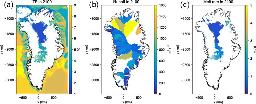
986                                                                 D. Slater et al.: Twenty-first century Greenland ocean forcing

2006; Khan et al., 2014; Murray et al., 2015). These tide-              that may be prevalent in summer (Motyka et al., 2003; Glad-
water glaciers are understood to have responded to climate              ish et al., 2015), fjord–shelf exchange driven by winds both
forcing occurring at their calving fronts, where the ice sheet          inside and outside of fjords (Jackson et al., 2014; Spall et al.,
meets the ocean (Nick et al., 2009; Luckman et al., 2015;               2017), and exchange due to variability in shelf water prop-
Wood et al., 2018). Thus, processes at the ice–ocean bound-             erties (Mortensen et al., 2014; Carroll et al., 2018). Once
ary and their representations in ice sheet models are a critical        warm water reaches the calving front, the transfer of heat
component of accurate future sea level projections.                     across the ice–ocean boundary layer is promoted by the near-
   The Ice Sheet Model Intercomparison Project (ISMIP6;                 ice circulation (Holland and Jenkins, 1999). During summer,
Nowicki et al., 2016) is the community-leading effort pro-              the release of ice sheet meltwater into fjords from beneath
jecting future sea level contribution from the Greenland and            tidewater glaciers drives localised but vigorous upwelling
Antarctic ice sheets for the upcoming Sixth Assessment                  plumes, which are thought to drive rapid submarine melting
Report of the Intergovernmental Panel on Climate Change                 (Mankoff et al., 2016; Sutherland et al., 2019). These plumes
(IPCC AR6). ISMIP6 follows a history of similar initiatives,            may also fuel a fjord-wide circulation which enhances sub-
such as SeaRISE (Bindschadler et al., 2013; Nowicki et al.,             marine melting over the full calving front (Slater et al., 2018;
2013a, b) and ice2sea (Gillet-Chaulet et al., 2012; Goelzer             Kienholz et al., 2019). Submarine melting can shape the calv-
et al., 2013), aimed at bringing together a number of ice sheet         ing front, creating regions of undercut and overcut ice (Fried
models and scientists across disciplines to improve projec-             et al., 2019), which may in turn enhance iceberg calving and
tions of ice sheet mass loss. Compared to previous initiatives,         drive glacier retreat (Luckman et al., 2015; How et al., 2019).
ISMIP6 is the first such effort to be fully integrated within the       Greenland’s shelf and fjords, however, remain sparsely ob-
Coupled Model Intercomparison Project (CMIP6); CMIP6                    served, especially in winter, and we have very few obser-
being itself a model intercomparison exercise focused on the            vations of submarine melt rate. Similarly, significant uncer-
representation of climate in coupled Atmosphere and Ocean               tainty surrounds the dynamic impact of submarine melting
general circulation models (AOGCMs). The full details and               on calving due to the difficulty of making the necessary mea-
the experimental protocol of the ISMIP6 project can be found            surements close to dangerous calving fronts.
in Nowicki et al. (2016) and Nowicki et al. (2020), while the              Many of these processes can be captured by models at
Greenland ice sheet sea level projections can now be found in           the individual fjord or glacier scale. Cowton et al. (2016)
Goelzer et al. (2020). The present paper focuses specifically           and Fraser et al. (2018) have modelled fjord–shelf exchange
on one aspect of ISMIP6: the representation of ocean forcing            at Kangerlussuaq Fjord in south-eastern Greenland, while
in the simulations of the Greenland ice sheet. The aim is to            Carroll et al. (2017) modelled fjord water renewal driven
relate large-scale climate, as defined by the CMIP AOGCMs,              by subglacial discharge in an idealised domain. Plumes and
to an ocean boundary condition for the ice sheet models.                the near-ice circulation they generate have been captured by
   Ocean forcing of the Greenland ice sheet occurs at around            models focused on the part of the fjord within a few kilo-
300 approximately vertical glacier calving fronts around                metres of the calving front (Xu et al., 2012; Slater et al.,
Greenland and at several larger ice shelves and floating                2018). The impact of submarine melting on calving has been
ice tongues located in the far north. Ocean forcing is here             studied at high resolution in both idealised and realistic set-
broadly defined as melting of the ice–ocean boundary (here-             tings (Cowton et al., 2019; Ma and Bassis, 2019; Todd et al.,
after called submarine melting) and the impact of this melt-            2019). Yet, the model resolution in these studies, at ∼ 500 m
ing on calving and glacier retreat. The design of boundary              for the fjord simulations, ∼ 10 m for the plume simulations
conditions that represent ocean forcing must take into ac-              and ∼ 50 m for the calving simulations, is far smaller than the
count three sets of processes. First, the transport of ocean            ∼ 50 km resolution of AOGCMs (e.g. Watanabe et al., 2010)
heat from the far-field ocean to calving fronts across conti-           or ∼ 2 km resolution of Greenland ice sheet models (Goelzer
nental shelves and up long and narrow fjords. Second, the               et al., 2018). Even regional ocean models (e.g. Gillard et al.,
near-ice circulation that drives heat transfer through the ice–         2016) do not yet represent fjords and fjord processes. Thus,
ocean boundary. Third, the impact of submarine melting on               climate and ice sheet models do not have sufficient resolution
iceberg calving and glacier retreat.                                    to capture the processes that modulate the effect of the ocean
   Understanding of these key processes has advanced                    on the Greenland ice sheet.
through both observations and models. Considering the ob-                  At present, therefore, projecting the sea level contribution
servations, warm Atlantic-origin water is found on the con-             of the Greenland ice sheet requires that we parameterise ice–
tinental shelf around Greenland either due to transport from            ocean processes, but well-validated parameterisations are not
the deep ocean to the shelf, often in deep troughs, or due              readily available. While progress has been made in observing
to advection along the shelf by coastal currents (Sutherland            and modelling fjord circulation and fjord–shelf exchange, we
et al., 2013; Rykova et al., 2015; Schaffer et al., 2017). The          still lack simple parameterisations or box models that could
same waters are found adjacent to calving fronts (Straneo               represent these processes in an efficient fashion (i.e. without
et al., 2012) and may enter the fjords by numerous pro-                 resorting to computationally expensive hydrodynamic mod-
cesses, including a glacier-driven estuarine-type circulation           els). Conversely, parameterisations exist for the submarine

The Cryosphere, 14, 985–1008, 2020                                                            www.the-cryosphere.net/14/985/2020/
D. Slater et al.: Twenty-first century Greenland ocean forcing                                                                  987

melting induced by plumes (Rignot et al., 2016; Slater et al.,      rine melting (Slater et al., 2019) and is imposed on an ice
2016), but we still have few observations with which to vali-       sheet model through a time-variable ice mask, an approach
date these parameterisations (Sutherland et al., 2019). Lastly,     first suggested by Cowton et al. (2018). The submarine melt
the search for a universal calving law has a long history (e.g.     implementation instead provides ice sheet modelling groups
Benn et al., 2007), but as for submarine melting no calving         with fields of subglacial runoff and ocean properties together
parameterisation has undergone sufficient validation for con-       with a suggested parameterisation for estimating submarine
fident use.                                                         melt from these quantities. Since glacier retreat is given by
   Given the described process uncertainty, the small scale         a competition between frontal ice velocity, calving and sub-
of key processes and the current lack of parameterisations          marine melting, the retreat implementation heavily parame-
for these processes, projecting ocean-induced ice mass loss         terises ocean forcing by implicitly assuming that all quan-
from the Greenland ice sheet is very challenging. To date, at-      tities are proportional to submarine melt rate (Slater et al.,
tempts to project future ice discharge from tidewater glaciers      2019). The submarine melt implementation allows ice sheet
have often relied on extrapolation from a few glaciers to the       models to resolve the competition between velocity, calving
whole ice sheet (Goelzer et al., 2013; Nick et al., 2013; Peano     and melting, perhaps by implementing a calving law that de-
et al., 2017; Beckmann et al., 2019; Morlighem et al., 2019)        pends on submarine melt rate.
or have employed ad hoc methods to mimic the impact of                  Both implementations require a parameterisation for sub-
ocean forcing that are not easily relatable to climate warming      marine melting. Theoretical considerations suggest that melt
scenarios (Price et al., 2011; Bindschadler et al., 2013; Fürst     rates are controlled primarily by local ocean velocity and
et al., 2015). In a single ice sheet model, a significant advance   ocean thermal forcing, the latter defined as the difference
was recently made by Aschwanden et al. (2019), who ran full         between the in situ temperature and in situ freezing point
ice sheet projections that resolve tidewater glaciers and were      (Gade, 1979; Holland and Jenkins, 1999). Near-ice ocean
forced by estimated submarine melt rates, but many of the ice       velocities are thought to be highest inside vigorous plumes
sheet models taking part in ISMIP6 do not currently have the        resulting from the emergence of buoyant subglacial runoff
resolution or technical capability for this approach (Goelzer       from the grounding line of the glacier (Mankoff et al., 2016).
et al., 2018).                                                      Submarine melt rate parameterisations (Jenkins, 2011; Xu
   Despite the described difficulties, we present a strategy for    et al., 2013; Slater et al., 2016), therefore, typically include
simulating the impact of the ocean on the ice sheet that will       the basic ingredients of subglacial runoff (Q) and ocean ther-
enable a suite of Greenland ice sheet models of diverse capa-       mal forcing (TF). In the retreat implementation, we follow
bilities to be systematically forced by future warming scenar-      Slater et al. (2019) in assuming that submarine melting is
ios (Goelzer et al., 2020). We do not aim to solve the prob-        proportional to Q0.4 TF and retreat (1L, in km) is propor-
lems of process understanding, scale and parameterisation           tional to submarine melting so that retreat may be estimated
but rather to offer a pragmatic approach based on the current       as
state of knowledge. This approach draws on existing param-
eterisations for tidewater glacier retreat (Slater et al., 2019)    1L = κ 1(Q0.4 TF),                                          (1)
and submarine melting (Rignot et al., 2016). The paper pro-
                                                                    where Q is the mean summer (June–July–August) subglacial
ceeds as follows. An overview of the two-tiered strategy for
                                                                    runoff (in m3 s−1 ) and TF is the ocean thermal forcing (in
ocean forcing is given, and the subglacial runoff and ocean         ◦ C). Slater et al. (2019) calibrated the linear coefficient κ
thermal forcing datasets are described. These time series are
                                                                    at nearly 200 tidewater glaciers by considering observed re-
combined into projections of glacier retreat and submarine
                                                                    treat, estimated subglacial runoff and observed ocean ther-
melting. We finally discuss the projected ocean forcing, its
                                                                    mal forcing over the time period 1960–2018. This resulted
temporal evolution, and spatial and inter-model variability.
                                                                    in a distribution for κ (in units km (m3 s−1 )−0.4 ◦ C−1 ) hav-
                                                                    ing a median κ50 = −0.17 and quartiles κ25 = −0.37 and
                                                                    κ75 = −0.06, respectively.
2     Methods                                                          For the submarine melt implementation, we follow Rignot
                                                                    et al. (2016) in parameterising submarine melt rate (ṁ) as
2.1    Overview
                                                                    ṁ = (3 · 10−4 h q 0.39 + 0.15) TF1.18 ,                    (2)
We develop two possible implementations for ocean forc-
ing of Greenland ice sheet models, referred to as the re-           where h is grounding line depth (in m), TF is the ocean
treat implementation and the submarine melt implementation          thermal forcing (in ◦ C) and q is the annual mean subglacial
(Fig. 1). The retreat implementation is designed to be imple-       runoff normalised by calving front area (in m d−1 ). We ac-
mentable by all of the ice sheet models taking part in ISMIP6       knowledge the inconsistency of using summer runoff for the
regardless of resolution, model physics or spin-up procedure.       retreat implementation and annual runoff for the submarine
In this implementation, retreat of the ice–ocean boundary           melt implementation, but we emphasise that this makes no
is estimated as a linear function of parameterised subma-           practical difference since annual and summer runoff are very

www.the-cryosphere.net/14/985/2020/                                                         The Cryosphere, 14, 985–1008, 2020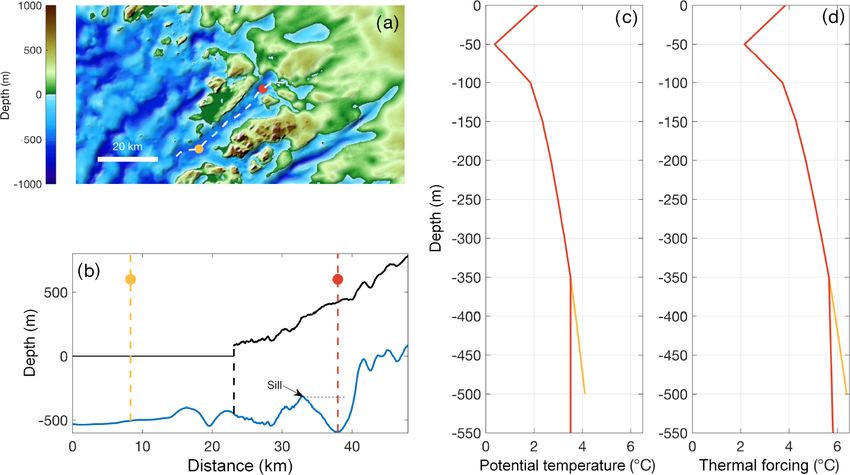
988                                                              D. Slater et al.: Twenty-first century Greenland ocean forcing

Figure 1. Schematic of proposed approach to use CMIP5 AOGCM output (top) to force Greenland ice sheet models (bottom) under the
retreat and submarine melt implementations described in the text. The coloured boxes describe the methodology and analysis performed in
this paper. Note that the process would be identical for CMIP6 models.

closely related, even in the future projections when the melt         icki et al., 2016). We also consider a single RCP2.6 sim-
season becomes longer (Slater et al., 2019). The parameter-           ulation (radiative forcing of 2.6 W m−2 in 2100). Each of
isation for submarine melting is slightly more complex than           the CMIP5 AOGCM simulations covers the period 1850-
that for retreat but is functionally very similar.                    2100, with 1850–2005 considered the historical spin-up pe-
   The chosen parameterisations require the two basic inputs          riod and the emissions forcing applied from 2006 to 2100
of future subglacial runoff and ocean thermal forcing, which          (Taylor et al., 2012). Ice sheet model ocean forcing is deliv-
are estimated from CMIP AOGCMs. While it is hoped that                ered for the time period from 1950 to 2100. The remainder
some of the new generation of climate models (CMIP6) will             of the Methods section describes the calculation of subglacial
be used in ISMIP6, very few CMIP6 simulations were avail-             runoff and ocean thermal forcing from AOGCM output and
able at the time of writing, and given the time constraints of        the combination of these datasets into ice sheet model ocean
the ISMIP6 project it was decided to focus largely on CMIP5,          forcing in the retreat and submarine melt implementations
for which the full ensemble is already available. We consider         (Fig. 1).
six CMIP5 AOGCMs (Table 1) that represent a subset of the
full CMIP5 ensemble but emphasise that the process would              2.2     Atmosphere
be identical for CMIP6 inputs. The six CMIP5 AOGCMs
have been chosen by selecting AOGCMs with minimal bi-                 2.2.1    Estimating ice sheet surface runoff using the
ases in the present day and with the aim of sampling the di-                   Modèle Atmosphérique Régional
versity of projected climate change, as described in Barthel
et al. (2019). The focus is on the RCP8.5 scenario, a high            Since the CMIP5 AOGCMs have a crude representation of
greenhouse gas emissions pathway in which radiative forc-             ice sheet surface mass balance, the Modèle Atmosphérique
ing reaches 8.5 W m−2 in 2100 (Riahi et al., 2011; Now-               Régional (MAR) is used to estimate surface runoff by down-

The Cryosphere, 14, 985–1008, 2020                                                          www.the-cryosphere.net/14/985/2020/
D. Slater et al.: Twenty-first century Greenland ocean forcing                                                                989

Table 1. CMIP5 AOGCMs and scenarios considered.                    scribed here (Jackson and Straneo, 2016; Mankoff et al.,
                                                                   2016; Jackson et al., 2017).
             Model              Scenario
             MIROC5             RCP2.6 & RCP8.5                    2.2.3   Present-day bias correction
             NorESM1-M          RCP8.5
             HadGEM2-ES         RCP8.5                             Many CMIP5 AOGCMs deviate considerably from the ob-
             CSIRO-Mk3.6.0      RCP8.5                             served present-day climate in both the atmosphere and ocean.
             IPSL-CM5A-MR       RCP8.5                             For example, Menary et al. (2015) show CMIP5 ocean tem-
             ACCESS1-3          RCP8.5                             perature biases can exceed 2 ◦ C in the Labrador Sea. If the
                                                                   AOGCM-simulated atmosphere is substantially colder than
                                                                   observations, runoff will be underestimated in MAR when
scaling the CMIP5 AOGCM atmospheric fields (Fig. 1; Fet-           forced by the AOGCM in question (Fettweis et al., 2013).
tweis et al., 2013). The most recent version of the model,         Since in the ISMIP6 exercise we wish to sample uncertainty
MAR 3.9.6, is run at 15 km resolution with surface mass bal-       in future projections rather than the representation of the
ance components (including runoff) statistically downscaled        present day, we perform a bias correction of the projected
afterwards to 1 km (Franco et al., 2012) to better account for     subglacial runoff at each glacier to ensure it agrees with our
sub-grid topography (Fig. 2a). Each simulation is forced at        best estimate of present-day runoff (Fig. 1). This bias correc-
its boundaries by 6-hourly output from a CMIP5 AOGCM               tion furthermore ensures a continuous transition from present
(Table 1) over the period 1950–2100.                               to future forcing, which is desirable as the ice sheet mod-
                                                                   els have been initialised to the present-day forcing (Goelzer
2.2.2   Hydrological drainage basins                               et al., 2018).
                                                                      Present day is defined as the time period 1995–2014. For
Both the retreat and submarine melt implementations use an         our best estimate of runoff in the present day we use a 5.5 km
estimate of subglacial runoff per tidewater glacier, which re-     resolution regional climate simulation using RACMO2.3p2,
quires a hydrological drainage basin for each glacier (Fig. 1).    forced at its boundaries by ERA-Interim atmospheric reanal-
These basins are delineated based on the hydrological poten-       ysis (Noël et al., 2018). We ensure that the projected runoff
tial (Shreve, 1972):                                               (QPROJ ) agrees with the RACMO runoff (QRACMO ) in the
                                                                   present day by bias-correcting the projected runoff for each
φ = ρw gb + f ρi gh,                                        (3)    glacier (j ) as follows:

where ρw = 1000 kg m−3 and ρi = 910 kg m−3 are the den-            QPROJ
                                                                    j    (t) → QPROJ
                                                                                j    (t)+
sities of freshwater and ice, respectively, and g = 9.81 m s−2      h                                        i
is the gravitational acceleration. Bed topography, b (m), and         QRACMO
                                                                       j      (1995–2014) − QPROJ
                                                                                             j    (1995–2014) ,               (4)
ice thickness, h (m), come from BedMachine v3 (Morlighem
et al., 2017). The variable f represents the ratio of subglacial   where the 1995–2014 in parentheses indicates the mean
water pressure to ice overburden pressure. Based on lim-           value between 1995 and 2014. We assume that the bias
ited borehole pressure records we set f = 1 (Meierbachtol          remains constant in time. An example of this procedure
et al., 2013; Andrews et al., 2014; Doyle et al., 2018) but        for Helheim Glacier in SE Greenland under MIROC5 in
acknowledge that different values of f can alter drainage          an RCP8.5 scenario is shown in Fig. 2c. In this case the
pathways (e.g. Chu et al., 2016; Moyer et al., 2019). By           JJA runoff estimated from MAR forced by MIROC5 is de-
performing flow routing on φ (Schwanghart and Scherler,            creased by 55 to 316 m3 s−1 to bring it into agreement with
2014), we identify the area of the ice sheet that drains sub-      the temporally averaged RACMO2.3p2 output over the pe-
glacial water to a given tidewater glacier calving front, defin-   riod 1995–2014. Note that we do not expect the interan-
ing hydrological drainage basins for each tidewater glacier        nual runoff variability in MAR forced by MIROC5 to agree
around the ice sheet (Fig. 2b). For simplicity the hydro-          with RACMO2.3p2 forced by ERA-Interim (Fig. 2c, inset)
logical drainage basins are assumed to be constant in time.        because MIROC5 is a free-running climate model whereas
Given the high density of moulins observed around the mar-         ERA-Interim is an atmospheric reanalysis.
gins of the ice sheet during summer (e.g. Yang and Smith,             Over all glaciers and all CMIP5 AOGCMs considered (Ta-
2016), we assume that all surface meltwater drains to the          ble 1), the mean bias correction is +2 m3 s−1 with a standard
ice sheet bed close to where it melts. The subglacial runoff       deviation of 56 m3 s−1 and a minimum and maximum cor-
for each glacier can then be estimated by summing the sur-         rection of −527 and +519 m3 s−1 , respectively (Fig. S1 in
face runoff from MAR over the hydrological drainage basin          the Supplement). As a fraction of the present-day runoff, the
for each glacier (Fig. 2b). Studies that have assessed sub-        mean bias correction is +0.13 with a standard deviation of
glacial runoff from fjord observations find agreement be-          0.47. Bias corrections for the largest glacier by ice flux in
tween their oceanographic estimates and the method de-             each sector and for all models are shown in Fig. S1.

www.the-cryosphere.net/14/985/2020/                                                      The Cryosphere, 14, 985–1008, 2020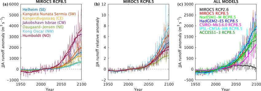
990 D. Slater et al.: Twenty-first century Greenland ocean forcing
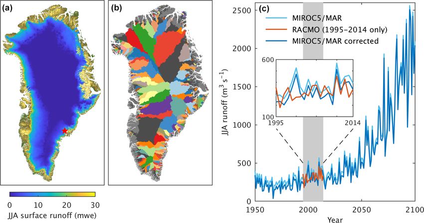
Figure 2. Illustration of atmospheric processing for the MIROC5 RCP8.5 scenario. (a) Simulated June–July–August (JJA) surface runoff in
2100 in the regional climate model MAR3.9.6 forced at its boundaries by MIROC5. (b) Tidewater glacier drainage basins delineated based
on the hydropotential defined in Eq. (3). (c) JJA runoff time series for Helheim Glacier in SE Greenland (location shown as red star in a).
The vertical grey shading shows the 1995–2014 present-day time period used for the bias correction. The raw MAR output is in light blue,
RACMO during the present-day period is in red and the bias-corrected MAR output is in dark blue. The inset shows the present-day time
period.
It would be better to use MAR forced by ERA-Interim for 2.3.2 Choice of ice–ocean sectors and spatial averaging
our best estimate of present day because it is MAR that is
used for the forward projections. If we define the interannual The ice sheet and surrounding ocean were divided into seven
runoff variability as the standard deviation of the detrended ice–ocean sectors (Fig. 3a), over which ocean properties
projections, we find a mean interannual variability across all were spatially averaged (Fig. 1). Each sector is hereafter re-
glaciers and AOGCMs of 74 m3 s−1 . Given that the bias cor- ferred to by its acronym (Fig. 3a), where SW is south-western
rection (i.e. the difference between RACMO and MAR in the Greenland, CW is central-western Greenland, NW is north-
present day) is typically smaller than the interannual variabil- western Greenland, NO is northern Greenland (and similarly
ity of the projections, the use of RACMO for the present day named equivalents on the eastern side of the ice sheet, i.e.
does not cause any inconsistency in practice. NE, CE and SE). The sectors, identical to those considered
in Slater et al. (2019), were chosen as regions with similar
2.3 Ocean ocean properties largely defined by ocean bathymetry (e.g.
Denmark, Fram and Nares straits) and consistent with the
2.3.1 Defining ocean thermal forcing boundaries of commonly used ice sheet drainage basins (e.g.
Mouginot et al., 2019) once extended into the ice sheet (see
Due to a lack of parameterisations that can capture fjord– Slater et al., 2019, for a more in depth description). The
shelf exchange and fjord circulation without resorting to full small region in CE Greenland is a transition zone between
hydrodynamic models, we take a simplified approach to es- the warm Atlantic waters in the Irminger Sea to the south
timating ocean thermal forcing in which the forcing experi- and cool Arctic waters in the Nordic Seas to the north and, as
enced by the glacier is directly related to far-field ocean prop- such, was split from the SE and NE Greenland sectors. Each
erties. As such, we are hardwiring tidewater glaciers to re- ice–ocean sector extends to the centre of the offshore ocean
spond to large-scale ocean changes at the expense of most of basin or strait, except for in the Arctic Ocean, Greenland Sea
the local details that we cannot currently account for. Specif- and Labrador Sea, where the ocean basin is very large and the
ically, we spatially average ocean properties over predefined sector boundary is located approximately 150 km beyond the
ocean regions and use these properties to force all tidewa- shelf break (Fig. 3). With these choices we sample the wa-
ter glaciers in the same region (Fig. 1). For the retreat im- ter masses that interact with the ice sheet but not those that
plementation, the far-field ocean properties are furthermore are recirculating (e.g. in western Baffin Bay). Extending the
depth-averaged (Sect. 2.4.1), while for the submarine melt sectors beyond the shelf break also allows us to access many
implementation, the far-field ocean properties are extrapo- more ocean observations (Fig. S2), which provides greater
lated into fjords taking account of bathymetry (Sect. 2.5.1). confidence in the calibration of the retreat parameterisation
The Cryosphere, 14, 985–1008, 2020 www.the-cryosphere.net/14/985/2020/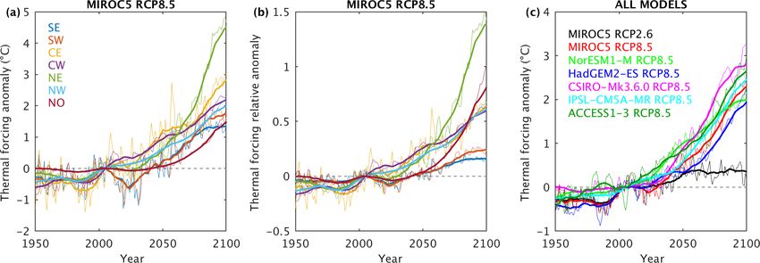
D. Slater et al.: Twenty-first century Greenland ocean forcing 991
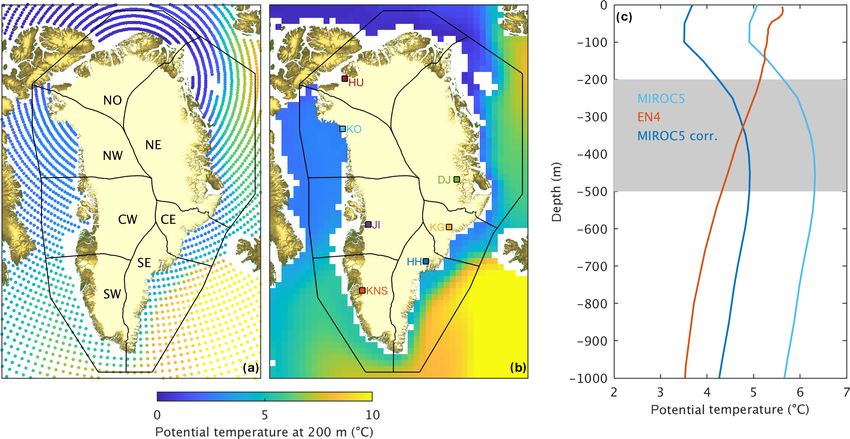
Figure 3. Illustration of ocean processing for the model MIROC5 in an RCP8.5 scenario. (a) Modelled annual mean potential temperature at
200 m in the year 2100, plotted at the 1.4◦ resolution of the climate model. The seven ice–ocean sectors over which properties are averaged
are also shown and labelled. (b) The same variable, gridded at 50 km resolution for spatial averaging. Also shown are the largest glaciers by
ice flux in each sector: HH (Helheim), KNS (Kangiata Nunata Sermia), KG (Kangerlussuaq), JI (Jakobshavn Isbræ), DJ (Daugaard-Jensen),
KO (Kong Oscar) and HU (Humboldt). (c) Ocean temperature bias correction for the SE sector. All three profiles are temporal averages
over the 1995–2014 present-day period. The raw MIROC5 output (light blue) is compared to the observational (EN4) profile (red) and is
bias-corrected (dark blue) so that the depth average over the 200–500 m range (shaded grey) agrees with EN4.
(Slater et al., 2019) and the bias correction (Sect. 2.3.3). ocean surrounding Greenland by oceanographic profiles in
Furthermore, the CMIP5 AOGCM ocean components have EN4 during the 1995–2014 present-day period is shown in
a coarse resolution of 20 to 100 km around Greenland (e.g. Fig. S2 and indicates that the SE, SW, CE and NE Greenland
Fig. 3a) and so may not resolve the details of ocean basin to sectors are relatively well observed, while the CW, NW and
shelf exchange and may have only a few model points on the NO Greenland sectors are sparsely sampled. As such, there
continental shelf. By extending the sectors beyond the shelf, is some uncertainty in present-day ocean properties which
we are allowing the ice sheet ocean forcing to respond to can feed through to uncertainty in retreat and submarine melt
larger-scale ocean features which may be better resolved by projections (Sect. 4.3).
the CMIP5 AOGCMs. We obtain annual profiles per ice–ocean sector from EN4
To obtain sector ocean properties, monthly CMIP5 in the same fashion as for the CMIP5 AOGCM projected
AOGCM outputs of modelled ocean potential temperature profiles. While for subglacial runoff we bias-corrected a sin-
(T ) and practical salinity (S) are first temporally averaged gle value, here we must bias-correct a whole temperature or
to annual means (Fig. 3a). Temperature and salinity are then salinity profile. Rather than applying a different bias correc-
linearly interpolated onto a regular grid with 50 km spatial tion at each depth level, we apply a single bias correction
and 50 m depth resolution (Fig. 3b). Sector ocean properties to the whole profile based on the observed bias in the 200–
are finally obtained by taking a simple spatial average over 500 m depth range. Specifically, we bias-correct ocean tem-
all regular grid points inside a given sector to give a single perature (Fig. 3c) as follows:
temperature and salinity profile for each ice–ocean sector for
each year (e.g. Fig. 3c). TiPROJ (z, t) → TiPROJ (z, t)+
h
TiEN4 (200–500 m, 1995–2014)
2.3.3 Present-day bias correction i
− TiPROJ (200–500 m, 1995–2014) . (5)
As for the subglacial runoff, we bias-correct the ocean prop-
erties to ensure consistency with observations in the present Here, TiPROJ (z, t) is the projected ocean temperature from the
day (Fig. 1). Observations of ocean properties are taken from CMIP5 AOGCM in ice–ocean sector i at depth z and in the
the Hadley Centre EN4.2.1 dataset (Good et al., 2013), here- year t. TiEN4 (200–500 m, 1995–2014) is the observed ocean
after called EN4. EN4 is a compilation of oceanographic temperature in EN4 in sector i, depth-averaged between
profile data, interpolated onto a monthly 1900–present grid- 200 and 500 m and temporally averaged over the 1995–
ded product available at 1◦ resolution. The coverage of the 2014 present-day period. TiPROJ (200–500 m, 1995–2014) is
www.the-cryosphere.net/14/985/2020/ The Cryosphere, 14, 985–1008, 2020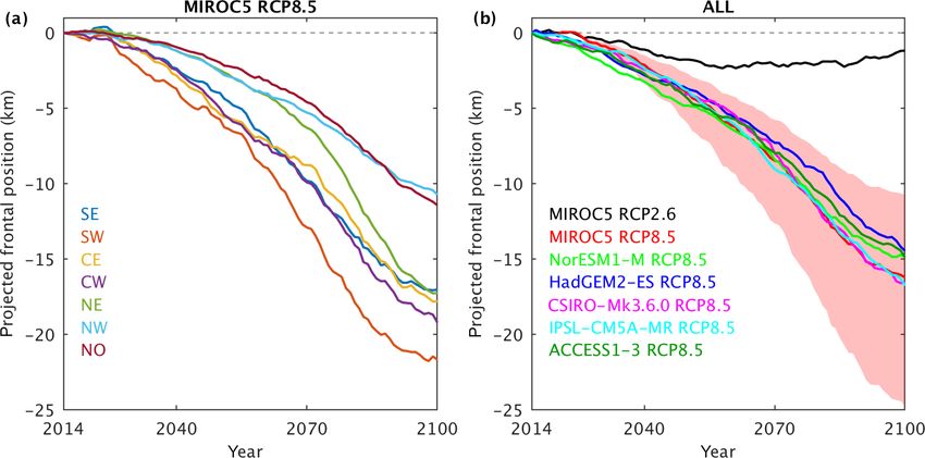
992                                                                D. Slater et al.: Twenty-first century Greenland ocean forcing

the projected ocean temperature from the CMIP5 AOGCM                   the glacier j is situated (Fig. 4a). Since this time series has
in sector i, averaged between 200 and 500 m depth and                  high interannual variability and for ISMIP6 we are most in-
over the present-day period. Salinity is bias-corrected in ex-         terested in the multi-decadal sea level contribution, the time
actly the same fashion. Since the vertical structure of the            series is smoothed using a 20-year centred moving aver-
ocean can vary in time in the CMIP5 AOGCMs, we felt a                  age (Fig. 4a). Lastly, in the CMIP6 and ISMIP6 frameworks
depth-varying bias correction could lead to unphysical pro-            (Nowicki et al., 2016; Eyring et al., 2016) the projections be-
files and that a single-valued correction, centred over the            gin in 2015 and we project retreat relative to 2014. Thus, for
depth range most relevant to tidewater glacier grounding               each glacier j , projected retreat 1Lj (t) is given by
lines (Morlighem et al., 2017), was preferable. As for the                          h                                             i
runoff, the bias correction is assumed constant in time. The           1Lj (t) = κ Q0.4 j  TF  i(j ) (t) − Q0.4
                                                                                                            j   TFi(j ) (t = 2014)  , (7)
magnitude of these corrections can be significant. For exam-
ple, in MIROC5 RCP8.5 the temperature bias correction for              where both terms on the right-hand side refer to the smoothed
SE Greenland is 1.4 ◦ C (Fig. 3c). Over all sectors and CMIP5          time series. We generate 104 possible future retreat trajecto-
AOGCMs considered, the mean temperature bias correction                ries for each glacier (Fig. 4b) by sampling 104 values of κ
is +0.1 ◦ C with a standard deviation of 1.5 ◦ C and a mini-           from its distribution obtained from observations (Slater et al.,
mum and maximum correction of −3.1 and +3.2 ◦ C, respec-               2019).
tively (Fig. S3).
                                                                       2.4.3   Averaging retreat per ice–ocean sector
2.4     Retreat implementation
                                                                       Due to limitations of the retreat parameterisation, principally
2.4.1    Calculation of ocean thermal forcing                          its lack of ability to capture individual glacier effects related
                                                                       to bed topography, it is most appropriate to apply retreat av-
To calculate the thermal forcing that enters the retreat pa-           eraged over a population of glaciers rather than on an indi-
rameterisation in Eq. (1), profiles of ocean temperature and           vidual glacier basis (Slater et al., 2019). From the ice sheet
salinity (e.g. Fig. 3c) are first converted to profiles of ther-       model perspective, this is also preferable because the state
mal forcing (Fig. 1). The thermal forcing (TF) is for the re-          of the ice sheet may differ significantly from the observed
treat parameterisation defined as the elevation of the potential       ice sheet (Goelzer et al., 2018). Thus, identifying individual
ocean temperature T above its local freezing point Tf                  glaciers in a given ice sheet model is not trivial, thus apply-
                                                                       ing retreat to individual glaciers is also difficult. An obvious
TFi (z, t) = Ti (z, t) − Tf,i (z, t) =
                                                                       solution is to impose a given retreat over a predefined geo-
  Ti (z, t) − [λ1 Si (z, t) + λ2 + λ3 z] ,                  (6)        graphical region (or ice–ocean sector), which means averag-
                                                                       ing retreat over a population of glaciers.
where in the second equality we have employed a linearised                A potential issue is that under the retreat parameterisation
expression for the local freezing point in terms of the prac-          (Eq. 1) glaciers with large hydrological catchments (typically
tical salinity S and depth z and the constants take values             glaciers such as Jakobshavn Isbræ or Helheim) undergo large
λ1 = −5.73×10⁻² ◦ C psu−1 , λ2 = 8.32×10⁻² ◦ C and λ3 =                changes in subglacial runoff and have large projected retreat
7.61×10⁻⁴ ◦ C m−1 (Jenkins, 2011). As before, i indexes the            relative to smaller glaciers. This is considered an important
ice–ocean sector.                                                      feature of the retreat parameterisation (Slater et al., 2019).
   In keeping with the simple philosophy of the retreat pa-            Each ice–ocean sector (Fig. 3a) typically has a small number
rameterisation, the profiles of thermal forcing TFi (z, t) are         of large glaciers and a large number of small glaciers, such
finally depth-averaged between 200 and 500 m depth, this be-           that taking a simple mean of the projected retreat over the
ing the depth range most relevant to tidewater glacier ground-         glaciers in a sector will result in a trajectory that is much
ing lines in Greenland (Morlighem et al., 2017). The final             closer to that of the small glaciers than the large glaciers.
thermal forcing entering Eq. (1) in the retreat implementa-            This is problematic because the primary objective of ISMIP6
tion is a single value per ice–ocean sector per year, for each         is sea level contribution and for Greenland this is dominated
CMIP5 model considered (Table 1).                                      by the largest glaciers (Enderlin et al., 2014). To address this
                                                                       problem, we take an ice-flux-weighted mean over glaciers in
2.4.2    Glacier-by-glacier projection of retreat
                                                                       a sector (Fig. 1). Specifically, we define the retreat for each
For each CMIP5 AOGCM we first estimate retreat for each                sector i as
of the 191 individual tidewater glaciers considered in Slater                      X               X
                                                                       1Li (t) =       fj 1Lj (t) / fj ,                             (8)
et al. (2019) by employing Eq. (1) with the summer sub-                           j ∈i             j ∈i
glacial runoff Q per glacier (Sect. 2.2) and ocean thermal
forcing TF per sector (Sect. 2.4.1). Specifically, for each            where fj is the 2000–2010 mean observed ice flux (Ender-
glacier j from 1 to 191 we form the time series Q0.4
                                                   j TFi(j ) ,         lin et al., 2014; King et al., 2018) and the sum runs over all
where i(j ) is the ice–ocean sector i from 1 to 7 in which             glaciers j in ice–ocean sector i. This ensures that the largest

The Cryosphere, 14, 985–1008, 2020                                                           www.the-cryosphere.net/14/985/2020/
D. Slater et al.: Twenty-first century Greenland ocean forcing 993
Figure 4. Illustration of retreat implementation processing for MIROC5 under an RCP8.5 scenario. (a) Time series of Q0.4 TF for Helheim
Glacier in SE Greenland, showing annual and 20-year centred mean smoothed values. (b) Projected retreat for Helheim Glacier; the solid
line is the median retreat while the shading denotes the interquartile range of all 104 derived retreat trajectories. (c) Projected retreat for the
SE ice–ocean sector. The dotted line shows the median of the trajectories obtained by taking a simple mean over glaciers, while the solid line
and shading show the median and interquartile range of the trajectories obtained by taking an ice-flux-weighted mean over glaciers.
glaciers are treated as the most important when generating a on the BedMachine v3 topography (Morlighem et al., 2017).
retreat projection per sector. Since we have 104 retreat tra- Specifically, for each location in a fjord and beneath the
jectories for each glacier (Fig. 4b), this procedure produces present-day ice sheet, the deepest point that is openly con-
an ensemble of 104 ice-flux-weighted retreat trajectories for nected to the wider ocean is determined; this depth is here-
each ice–ocean sector. As expected, the median retreat of this after termed the effective depth. Water shallower than the ef-
ice-flux-weighted ensemble is larger than the median retreat fective depth is assumed to communicate directly with the
that would have been obtained by taking a simple mean over open ocean and is assigned the temperature and salinity pro-
glaciers in a sector (Fig. 4c). file for the sector in question. Water deeper than the effective
depth is not in direct communication with the open ocean be-
2.4.4 Low, medium and high scenarios cause there is no continuous path to the open ocean that is not
blocked by shallower bathymetry. Water deeper than the ef-
Given the large uncertainty associated with tidewater glacier fective depth is, therefore, uniformly assigned a temperature
response to climate forcing and the need to quantify uncer- and salinity equal to that at the effective depth.
tainties on future sea level contributions, it is desirable to pro- An illustrative example is given for Sverdrup Glacier in
vide a range of projected retreat that brackets the uncertainty NW Greenland and the adjacent ocean (Fig. 5). The fjord
associated with the retreat implementation. For each CMIP5 mouth has full-depth open communication with the ocean
AOGCM we identify a low-, medium- and high-retreat sce- and is assigned unmodified ocean properties for the NW sec-
nario (Fig. 1). From the ensemble of 104 ice-flux-weighted tor (yellow profiles in Fig. 5b–d). The bed topography at a
retreat trajectories for each ice–ocean sector, we define the point beneath the present-day ice sheet reaches 600 m be-
medium retreat scenario as the trajectory with the median re- low sea level but, assuming that the glacier had retreated past
treat at 2100 and the low- and high-retreat scenarios as the this point, would be separated from the open ocean by a sill
trajectories with the 25th and 75th percentile retreats at 2100 at ∼ 350 m depth (Fig. 5a and b). By our extrapolation, this
(Fig. 4c). 600 m deep region is isolated from the warmest and saltiest
water on the continental shelf. Thus, the ocean properties in
2.5 Submarine melt implementation this deep region (red profiles in Fig. 5b–d) diverge from those
at the fjord mouth below the height of the sill. This procedure
2.5.1 Extrapolation of ocean properties into fjords is repeated for all fjords around the ice sheet, including be-
low the present-day ice sheet so that ocean conditions at calv-
In the submarine melt implementation, we account for the ing fronts will be available to ice sheet models after calving
effects of fjord bathymetry and grounding line depth on the fronts have retreated.
thermal forcing experienced by the glacier (Fig. 1). This is
achieved by extrapolating the ocean property profiles (e.g. 2.5.2 Calculation of ocean thermal forcing
Fig. 3c) into fjords and below the present-day ice sheet by
taking into account ocean bathymetry and subglacial topog- In line with the more complex nature of the submarine
raphy in the same manner as Morlighem et al. (2019), based melt implementation relative to the retreat implementation
www.the-cryosphere.net/14/985/2020/ The Cryosphere, 14, 985–1008, 2020994 D. Slater et al.: Twenty-first century Greenland ocean forcing
Figure 5. Illustration of ocean property extrapolation for Sverdrup Glacier and fjord, NW Greenland. (a) Overview of regional topography.
The dashed white line shows an along-fjord transect, the yellow point is in the fjord and the red point is below the present-day ice sheet.
(b) Bathymetry and subglacial topography (blue) and current ice sheet elevation (black) along the flow line shown as the dashed white line
in (a). The dashed yellow and dashed red lines correspond to the locations in (a). (c) Potential temperature profiles and (d) thermal forcing
profiles at the locations shown in yellow and red in (a) and (b).
we use full, non-linear TEOS-10 routines (McDougall and 2.5.3 Assignation of runoff to drainage basins
Barker, 2011) to convert ocean property profiles to ocean
thermal forcing profiles (Figs. 1 and 5d). Specifically, the The treatment of subglacial runoff is initially the same as
CMIP5 quantities of depth, practical salinity and poten- for the retreat parameterisation. Once the time series of
tial temperature are converted to pressure, absolute salin- bias-corrected subglacial runoff has been obtained for each
ity and in situ temperature using the “gsw_p_from_z”, marine-terminating glacier (Sect. 2.2), this runoff is dis-
“gsw_SA_from_SP” and “gsw_t_from_pt0” routines, re- tributed onto a 1 km x–y grid by assigning the total runoff
spectively. A full three-dimensional, time-varying thermal for each hydrological basin (Fig. 2b) to every grid point ly-
forcing field TF(x, y, z, t) is obtained as ing inside the basin (Figs. 1 and 6b). In this way, as a calving
front retreats over the x–y grid, the calving front submarine
TF(x, y, z, t) = T (x, y, z, t) − Tf (x, y, z, t), (9)
melt rate may be obtained by sampling the ocean thermal
where T is the in situ temperature and Tf is the in situ forcing and subglacial runoff from the grid point at which the
freezing point that depends on pressure and absolute salin- calving front is currently located. We assume that the hydro-
ity as defined by the “gsw_t_freezing” routine. Lastly, we logical drainage basins remain fixed in time at their present-
collapse the three-dimensional thermal forcing field to two- day extent. Extending the runoff field beyond the present-day
dimensions by considering only the value at the ocean bottom ice sheet is desirable to allow for potential calving front ad-
so that the final thermal forcing field (TF) is defined at annual vance in the simulations, or to accommodate models whose
resolution on a 1 km x–y grid covering Greenland (Fig. 6a). initial ice extent is larger than observations. We choose to
The motivation for using the ocean bottom value is that this extrapolate subglacial runoff values beyond the present-day
is the thermal forcing experienced by the grounding line of ice sheet by three 1 km grid cells using an iterative buffer-
a glacier if its calving front was located in the grid cell in ing approach. First, we sort the drainage basins by area from
question. Furthermore, plumes upwell deep waters towards largest to smallest. For each iteration, we buffer runoff val-
the fjord surface so that the temperature profile within the ues by a single 1 km grid cell around each basin, starting with
plume is well approximated by the value at the ocean bot- the largest basin and ending with the smallest basin. We fill
tom (Mankoff et al., 2016). We note that the submarine melt only empty grid cells such that if a grid cell has already been
parameterisation is non-linear in TF (Eq. 2) so that annual populated by a runoff value from a larger basin, we do not
mean melt is not equal to melt calculated from annual mean overwrite that value. In this way, grid cells that are adjacent
TF. The difference is, however, less than 1 % and it is, there- to two drainage basins are filled with runoff values from the
fore, justified to use annual mean TF. larger basin. After the third iteration, we are left with a field
The Cryosphere, 14, 985–1008, 2020 www.the-cryosphere.net/14/985/2020/D. Slater et al.: Twenty-first century Greenland ocean forcing 995
Figure 6. Example of forcing fields in 2100 in the submarine melt implementation, using MIROC5 under an RCP8.5 scenario. (a) Ocean
thermal forcing, (b) subglacial runoff and (c) submarine melt rate calculated using the parameterisation in Eq. (2). Note that the thermal
forcing and melt rate values in the ice sheet interior are included only to show that the submarine melt implementation defines melt rate
everywhere that is below sea level and connected to the ocean. An ice sheet model would only apply these melt rates if the ice sheet margin
retreats into the interior, which is unlikely by 2100. Also note that runoff values are only plotted for marine-terminating hydrological basins.
of annual cumulative basin runoff values that have been ex- varying submarine melt rate to calving fronts around the ice
trapolated by three 1 km grid cells beyond the present-day ice sheet as these calving fronts retreat over the coming century.
sheet extent.
The submarine melt parameterisation Eq. (2) takes as in-
put the subglacial runoff normalised by the submerged area 3 Results
of the calving front for each glacier. The submerged area will
change over the course of the ice sheet model simulations Here we present the Greenland ice sheet ocean forcing aris-
as the termini retreat through fjords of various depths and ing from the choices and steps made in Sect. 2. The inten-
widths. Since dynamically calculating the submerged area is tion is to highlight temporal evolution of the forcing, to-
difficult within an ice sheet model, we assume that the sub- gether with spatial and model-to-model variability, as these
merged area of each terminus remains constant at present- factors will drive variability in sea level projections once im-
day values (see Morlighem et al., 2019) but highlight this plemented in an ice sheet model. The results are discussed
as an area for improvement in future efforts. The present- with the same structure as Sect. 2 and Fig. 1.
day submerged surface area is calculated based on present-
day calving front position and bed topography as defined by 3.1 Future subglacial runoff
BedMachine v3 (Morlighem et al., 2017). Due to poor bed
topography in some regions, which typically means unreal- For both implementations, projected subglacial runoff is
istically shallow topography in the region of a calving front, prescribed for each tidewater glacier using its hydrological
we impose a minimum submerged surface area of 0.2 km2 , drainage basin. We visualise variability in runoff by consider-
equivalent to a glacier of 2 km width and a grounding line ing runoff for the largest glacier by ice flux in each sector (Ta-
depth of 100 m. ble S1; Fig. 3b), as these glaciers are likely to contribute the
most to sea level over the coming century. These glaciers are
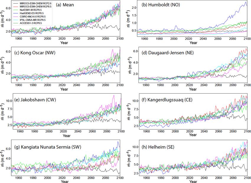
2.5.4 Application of submarine melt parameterisation Helheim (SE), Kangiata Nunata Sermia (SW), Kangerlus-
suaq (CE), Jakobshavn (CW), Daugaard-Jensen (NE), Kong
Armed with both ocean thermal forcing and subglacial runoff Oscar (NW) and Humboldt (NO); note that in the retreat im-
fields defined at annual resolution on 1 km grids and with plementation, glaciers that have permanent ice shelves have
the submarine melt rate parameterisation Eq. (2), submarine been excluded. Runoff shows high interannual variability and
melt rates may be estimated for the time period 1950–2100 so we also plot and discuss smoothed curves.
and for each CMIP5 model (Fig. 1 and Table 1). While this In the MIROC5 RCP8.5 simulation, all glaciers show a
defines a submarine melt rate on every grid cell where both significant increase in runoff by 2100, with most of the in-
ocean thermal forcing and runoff are defined (Fig. 6c), the crease occurring after 2050 (Fig. 7a). Jakobshavn (CW) and
intention is that the ice sheet model applies this submarine Humboldt (NO) show the largest absolute increase in runoff,
melt rate only when the model has a calving front within this with Daugaard-Jensen (NE) and Kong Oscar (NW) having
grid cell. In this way, the ice sheet models may apply a time- the smallest runoff anomaly (Fig. 7a). A different picture
www.the-cryosphere.net/14/985/2020/ The Cryosphere, 14, 985–1008, 2020996 D. Slater et al.: Twenty-first century Greenland ocean forcing
of spatial variability emerges when considering the rela- We consider ocean warming at the ice sheet scale by tak-
tive runoff anomaly (Fig. 7b). In this case it is Kong Os- ing a mean over the seven sectors for each CMIP5 AOGCM
car (NW) that stands out, with JJA runoff in 2100 a fac- (Fig. 8c). For MIROC5 RCP2.6, there is moderate warm-
tor of 8 larger than during the 1995–2014 baseline period. ing of nearly half a degree, which persists until the end of
Kangiata Nunata Sermia (SW) also experiences a large rel- the century. This is mostly driven by significant warming
ative increase in runoff, while Daugaard-Jensen (NE) sees in the CW and NW sectors (Fig. S6a) that exceeds warm-
the smallest, amounting to only a factor of 2.5 larger than in ing in these sectors in some of the RCP8.5 simulations
1995–2014. Equivalent plots for all other CMIP5 AOGCMs (Figs. S6d and f). Given the large inter-model variability
are shown in Figs. S4 and S5 but show very similar spatial in ocean warming, this warming feature is likely to be spe-
variability to MIROC5. cific to MIROC5 rather than being more broadly representa-
Lastly, we consider model-to-model variability in pro- tive of RCP2.6 simulations. Among the RCP8.5 simulations,
jected runoff by averaging over the largest glaciers by sec- CSIRO-Mk3.6.0 shows the most warming by 2100, reach-
tor (Fig. 7c). The only RCP2.6 scenario considered shows ing 2.8 ◦ C above the present-day value. HadGEM2-ES shows
a moderate increase in runoff until 2050 before a return the least warming, reaching 1.9 ◦ C by 2100. The multi-model
to present-day values by 2100 (Fig. 7c). All RCP8.5 sim- spread in thermal forcing anomaly by 2100 is 0.9 ◦ C, around
ulations exhibit a similar temporal evolution and show a 35 % of the multi-model mean of ∼ 2.4 ◦ C. Relative to the
significant increase in runoff during the coming century. 1995–2014 baseline value of 4.6 ◦ C, thermal forcing is pro-
HadGEM2-ES has the highest runoff at ∼ 2000 m3 s−1 in jected to increase by a factor of 0.4–0.6 this century under
2100, with IPSL-CM5A and MIROC5 giving similar re- RCP8.5 (Fig. 8c).
sults. NorESM1-M and ACCESS1-3 have medium runoff
and CSIRO-Mk3.6.0 has the lowest runoff at ∼ 1150 m3 s−1 3.3 Retreat implementation forcing
by 2100. The multi-model spread in runoff anomaly at 2100
is ∼ 850 m3 s−1 , around 50 % of the multi-model mean of ∼ Projected sector retreat combines the runoff anomaly per
1650 m3 s−1 . Relative to the 1995–2014 mean of 440 m3 s−1 , glacier (Sect. 3.1), the thermal forcing anomaly per sec-
these projections suggest an average increase in runoff by a tor (Sect. 3.2) and the ice flux of all glaciers in the sector
factor of 2.5–4.5 this century. The model-to-model variabil- (Sect. 2.4.3). Thus, sector-to-sector variability in projected
ity is as would be expected from the ISMIP6 CMIP5 model retreat arises due to both variability in regional climate and
evaluation exercise (Barthel et al., 2019). differences in the population of glaciers in each sector.
For the MIROC5 RCP8.5 simulation, the SW sector has
3.2 Future ocean thermal forcing the largest retreat (Fig. 9a) because it has a small number of
glaciers (Table S1), each experiencing a large increase in sub-
We present ocean results based on the sector-averaged, glacial runoff (Fig. 7a–b). The projected retreat for the CW
depth-averaged time series derived for the retreat implemen- sector is also high (Fig. 9a), partly due to large projected re-
tation (Sect. 2.4.1). While the submarine melt implementa- treat for Jakobshavn, which dominates the sector-average re-
tion differs by retaining depth variability and through the ex- treat because it alone accounts for around half of the present-
trapolation of properties into fjords, the depth-averaged val- day ice flux in the CW sector (Table S1). Projected retreat
ues from the retreat implementation remain a reliable indica- is smallest for the NW and NO sectors (Fig. 9a) because
tor of what the ocean does. these sectors comprise a large population of smaller glaciers
There is significant regional variability in projected ocean (Table S1) and experience the least absolute increase in sub-
warming in the MIROC5 RCP8.5 simulation (Fig. 8a). The glacial runoff (Fig. 7a). Figure S8 shows equivalent plots to
NE sector stands out with a thermal forcing increase of nearly Fig. 9a for all other CMIP5 AOGCMs, in which the spatial
5 ◦ C, while all other sectors exhibit an increase of between 1 patterns of retreat are similar in almost all models with large
and 3 ◦ C. Ocean warming in the NE sector amounts to an projected retreat for SW and CW and smaller retreat for NW
increase of 150 % in thermal forcing relative to the 1995– and NO. Note that Fig. 9a shows only the medium retreat
2014 baseline period (Fig. 8b). The SE and SW sectors see case for each sector; low and high projections are plotted in
the smallest relative increase, amounting to only ∼ 20 %. We Fig. S9.
do note, however, that regional ocean warming differs sub- To provide an ice-sheet-wide view of retreat per CMIP5
stantially across CMIP5 AOGCMs (Yin et al., 2011; Barthel AOGCM, we combine the sector-by-sector projections (e.g.
et al., 2019, Figs. S6 and S7). The NE sector sees the most Fig. 9a) into an ice sheet projection by weighting accord-
warming in MIROC5, HadGEM2-ES and IPSL-CM5A-MR, ing to the present-day ice flux (Table S1). The resulting pro-
but the CW and NW regions see equivalent or greater warm- jections (Fig. 9b) are not used to force the ice sheet mod-
ing in the other three RCP8.5 models. It is also interest- els (the ice sheet models are forced by the sector-by-sector
ing to note that the relative increase in runoff (Fig. 7b) is projections), but they do illustrate multi-model variability in
much larger than the relative increase in ocean thermal forc- projected retreat. The RCP2.6 simulation considered shows
ing (Fig. 8b). moderate retreat of ∼ 2 km until 2050 and then a stabilisa-
The Cryosphere, 14, 985–1008, 2020 www.the-cryosphere.net/14/985/2020/You can also read


