Unconstrained Estimation of Multitype Car Rental Demand
←
→
Page content transcription
If your browser does not render page correctly, please read the page content below
applied
              sciences
Article
Unconstrained Estimation of Multitype Car Rental Demand
Yazao Yang 1, * , Avishai (Avi) Ceder 2 , Weiyong Zhang 1 and Haodong Tang 1

                                          1   College of Traffic & Transportation, Chongqing Jiaotong University, Chongqing 400074, China;
                                              zhang576612829@163.com (W.Z.); tanghaodong@mails.cqjtu.edu.cn (H.T.)
                                          2   Department of Civil and Environmental Engineering, Technion-Israel Institute of Technology,
                                              Haifa 32000, Israel; ceder@technion.ac.il
                                          *   Correspondence: yyzjt@cqjtu.edu.cn

                                          Abstract: The unconstrained demand forecast for car rentals has become a difficult problem for
                                          revenue management due to the need to cope with a variety of rental vehicles, the strong subjective
                                          desires and requests of customers, and the high probability of upgrading and downgrading circum-
                                          stances. The unconstrained demand forecast mainly includes repairing of constrained historical
                                          demand and forecasting of future demand. In this work, a new methodology is developed based on
                                          multiple discrete choice models to obtain customer choice preference probabilities and improve a
                                          known spill model, including a repair process of the unconstrained demand. In addition, the linear
                                          Holt–Winters model and the nonlinear backpropagation neural network are combined to predict
                                          future demand and avoid excessive errors caused by a single method. In a case study, we take
                                          advantage of a stated preference and a revealed preference survey and use the variable precision
                                          rough set to obtain factors and weights that affect customer choices. In this case study and based on
                                          a numerical example, three forecasting methods are compared to determine the car rental demand of
                                          the next time cycle. The comparison with real demand verifies the feasibility and effectiveness of the
                                          hybrid forecasting model with a resulting average error of only 3.06%.


                                          Keywords: transportation; demand estimation and forecasting; car rental; revenue management
Citation: Yang, Y.; Ceder, A.; Zhang,
W.; Tang, H. Unconstrained
Estimation of Multitype Car Rental
Demand. Appl. Sci. 2021, 11, 4506.
https://doi.org/10.3390/app11104506       1. Introduction
                                               The car rental industry plays a huge role globally. It can act as a lubricant for produc-
Academic Editor: Yosoon Choi              tion and consumption to ease their mutual restraints. It can also expand the automotive
                                          consumer market and evaluate the popularity of new cars before they come into the market.
Received: 24 April 2021                   At the same time, because the public transportation system is limited by operating time,
Accepted: 11 May 2021                     departure frequency, accessible range, comfort, privacy, and other conditions, car rental,
Published: 14 May 2021
                                          with its outstanding advantages such as high flexibility, ease of use, and privacy, has shown
                                          considerable growth over the years. The global car rental market was valued at $79.5 bn
Publisher’s Note: MDPI stays neutral
                                          in 2018 and is expected to reach $125.4 bn by 2025, registering a CAGR of 5.1% from 2019
with regard to jurisdictional claims in
                                          to 2025 [1]. In recent years, the demand for car rental services in the Asia-Pacific region
published maps and institutional affil-
                                          has become the largest and fastest growing segment, especially in China and India, where
iations.
                                          there are high population density and rapidly growing demand.
                                               Mainstream car rental companies started to use revenue management (RM) as a crucial
                                          tool for reducing operating costs and improving competitiveness in the 1990s. RM is an
                                          important interface between enterprises’ supply and market demand, and its objective is
Copyright: © 2021 by the authors.         to maximize profits. The most widely known RM application occurs in the airline industry.
Licensee MDPI, Basel, Switzerland.
                                          It mainly includes four aspects, namely forecasting, overbooking, capacity control, and
This article is an open access article
                                          pricing [2]. Among them, forecasting is the foundation and provides vital input information
distributed under the terms and
                                          for other work. A 12.5–25% reduction of forecast error could translate into 1–3% incremental
conditions of the Creative Commons
                                          revenue generated from the RM system [3,4]. Therefore, to achieve the desired level of
Attribution (CC BY) license (https://
                                          accuracy, it is important and necessary to innovate the forecast method constantly [5]. In
creativecommons.org/licenses/by/
                                          reality, influenced by booking and/or capacity limits, the customer’s present demand
4.0/).

Appl. Sci. 2021, 11, 4506. https://doi.org/10.3390/app11104506                                               https://www.mdpi.com/journal/applsci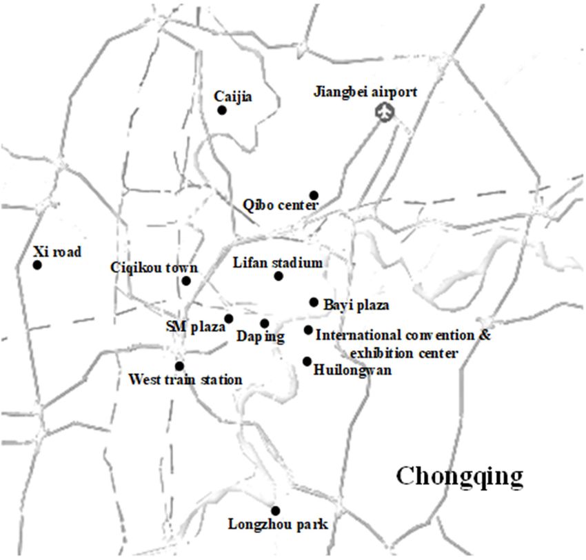
Appl. Sci. 2021, 11, 4506 2 of 28
Appl. Sci. 2021, 11, 4506 2 of 26
constantly [5]. In reality, influenced by booking and/or capacity limits, the customer’s pre-
sent
maydemand may not be
not be satisfied, satisfied,
which which
will lead to will lead lost
it being to it(spilled)
being lost or(spilled) or recaptured
recaptured by a more
by a more expensive (buyup) or cheaper (buydown) available product.
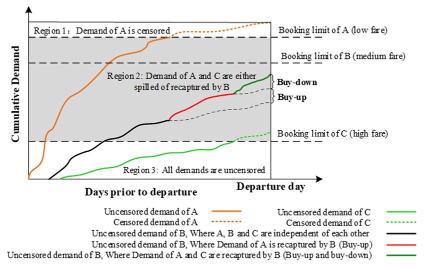
expensive (buyup) or cheaper (buydown) available product. The sample booking curves The sample book-
ing curves with three grades of products (the fare order is A > B > C) are shown
with three grades of products (the fare order is A > B > C) are shown in Figure 1 [6,7]. in Figure
1Therefore,
[6,7]. Therefore,
in orderin order to repair
to repair the constrained
the constrained demand,
demand, it is itnecessary
is necessary to carry
to carry outout
an
an unconstrained estimation of the customer’s actual demand and forecast
unconstrained estimation of the customer’s actual demand and forecast the future demand the future de-
mand onbasis
on this this [8,9].
basis [8,9].
Figure 1. Booking curves for given streams of arrivals.
Figure 1. Booking curves for given streams of arrivals.
Research into unconstrained estimation (sometimes also called detruncation, uncen-
Research
soring) in the into unconstrained
RM system estimation
started more than 40 (sometimes
years ago and alsomainly
called detruncation,
focused on theuncen- airline
soring) in the RM system started more than 40 years
industry. Unconstrained estimation mainly uses observed “censored demand”ago and mainly focused on totheestimate
airline
industry. Unconstrained
and calculate the “uncensoredestimation mainly The
demand”. usesoriginal
observed “censored
methods weredemand”
based on to estimate
statistics,
and calculate the “uncensored demand”. The original methods
such as the expectation maximization (EM), projection detruncation (PD), booking were based on statistics,
curve
such as the expectation maximization (EM), projection detruncation
(BC), and mean imputation. Since the beginning of this century, discrete customer choice (PD), booking curve
(BC),
modelsandhave
mean imputation.
grown Since to
in popularity theestimate
beginning of this century,
unconstrained demanddiscrete customer
[8,10,11]. choice
Forecasting
models have grown in popularity to estimate unconstrained
usually yields the demands and no-show rate by booking class, the latter of which will demand [8,10,11]. Forecast-
ing
notusually yields the
be discussed demands
here. The commonand no-show
methods rateinclude
by booking timeclass,
series,the latterregression,
linear of which will ex-
not be discussed here. The common methods include time series,
ponential smoothing, double exponential smoothing, pickup, neural networks, principal linear regression, expo-
nential
componentsmoothing,
analysis, double exponential
and adaptive models smoothing, pickup,
[6,12,13]. Since air neural networks,
transportation canprincipal
meet the
component
travel demand analysis,
between andtwoadaptive
points,models [6,12,13].
the prediction of Since
OD demandair transportation
is necessarycan meet Guo
[14–16]. the
travel demand
surveyed between
the history two points,
of research the prediction of
on unconstraining OD demand
methods is necessary
by reviewing over 130[14–16].
refer-
Guo
encessurveyed the historyprovided
[17]. Weatherford of research twoonreviews
unconstraining methods estimation
of unconstrained by reviewing andover 130
forecast
references [17]. Weatherford provided two reviews of unconstrained
methods broadly used in different industries up to 2016 [18,19]. Recent discussions include estimation and fore-
cast methods
forecast broadlyand
multipliers used in different
hybrid forecastingindustries
[9], theup to 2016
effect [18,19]. Recent
of customers’ discussions
reference price on
include
demandforecast multipliers
[20], Gaussian and hybrid
processes forecasting [9],demand
for unconstraining the effect of customers’
[21], and demand reference
forecast
price on demand
accuracy [22]. Due[20], Gaussian
to the important processes
researchfor andunconstraining
application value demand [21], and
of revenue demand
management
forecast accuracy
theory, many [22]. Due
advances have to been
the important
made in the research
hotel, andcar orapplication
truck rental,value of revenue
cargo/freight,
management
internet service theory,
and many advances
retailing, cruise have beenand
line, rail, made otherin the hotel, car
industries or truckdemand
regarding rental,
cargo/freight,
estimation and internet service
forecasting and retailing, cruise line, rail, and other industries regard-
[19].
Unlike estimation
ing demand the airline industry, the car rental
and forecasting [19]. industry is more concerned with the demand
at each rental
Unlike thestation,
airlineand OD forecasting
industry, the car rentaldoes not need to
industry is be considered
more concerned as much.
with the Supply
de-
and demand
mand at each are
rentaldynamically
station, and balanced, but theredoes
OD forecasting is still
notanneed
overestimation or underestima-
to be considered as much.
tion. Since
Supply and demand
demanddetermines
are dynamicallythe size of the leasing
balanced, station
but there inventory
is still and fleet, demand
an overestimation or un-
derestimation. Since demand determines the size of the leasing station inventory andoffleet,
estimation and forecasting techniques are worth studying [23]. The first reports RM
demand estimation and forecasting techniques are worth studying [23]. The first reportsa
application to car rental were at Hertz and National Car Rental [24,25]. Jishan used
decomposition
of RM application method to identify
to car rental werethe actualand
at Hertz latent demand
National Carfrom the [24,25].
Rental total recorded turn-
Jishan used
downs [26]. Gordon simplified the problem by human–computer interaction, hoping to
Appl. Sci. 2021, 11, 4506                                                                                                 3 of 26

                            find the right level of detail at which to forecast and optimize [27]. Dhruval optimized the
                            fleet with the help of a robust design methodology, considering fleet as a product and cars
                            as an affecting variable [28]. Kourentzes addressed the frequently encountered situation of
                            observing only a few sales events at the individual product level and proposed variants of
                            small demand forecasting methods to be used for unconstraining [29]. In general, there is
                            relatively little research on unconstrained estimation and prediction of car rental demand.
                            By referring to research methods in other fields, relevant research in the car rental industry
                            is worthy of a further discussion.
                                  Due to the relative lack of articles that deal with car rental demand forecasting, this
                            work develops an optimization methodology to estimate and forecast the demand for a car
                            rental station; it is then applied to a case study in China. By using the case study, the work
                            also enables comparison between the effects of different methods, especially for cases of
                            small demand. The remainder of this work is organized as follows. Section 2 presents the
                            problem statement and hypothesis, including an improved spill model for unconstrained
                            estimation. In Section 3, we propose a hybrid forecasting method based on the Holt–
                            Winters model and backpropagation neural network. Subsequently, Section 4 introduces
                            the case study with numerical experiments and a discussion. Section 5 concludes the work.

                            2. Unconstrained Estimation
                            2.1. Hypothesis and Variable Definitions
                                 Before studying the forecasting method, the conditional hypothesis and variable
                            definitions should be explained. This work is mainly aimed at the car rental industry, and
                            the method is also applicable to the hotel and aviation industries, etc.

                            Hypothesis 1. Unconstrained demand X of car type i in presell lead time meets normal distribution,
                            and the lead time is seven days.

                            Hypothesis 2. Demands of various car types are random and independent, and the numbers of car
                            rentals are counted by day; the deadline is midnight.

                            Hypothesis 3. Inventory quantity is constant without car dispatching among stations, taking no
                            account of batch demand, overdue return, or oversold behaviors.

                            Hypothesis 4. The customer’s willingness to pay is from low to high.

                                 The variables are defined as follows:
                            i: index of car types, i ∈ I. Indexes of I are listed in an increasing order of car rental price,
                            corresponding to the gradually increased levels;
                            j: index of rental demand recording times, j = 1, 2, · · · , J;
                            t: review points of inventory control, t = 0, 1, · · · , T; presale system will open when t = 0,
                            and it will be closed when t = T.
                            ∆t : presale lead time interval between t and t − 1;
                            B(i, j, t): order quantity limit of car type i in ∆t in the jth documented circle, namely the
                            quota ceiling for rent;
                            C (i, j, t): cumulative order quantity of car type i at review point t in the jth documented
                            circle, particularly C (i, j, 0) = 0;
                            I (i, j, t): presale state of car type i in ∆t in the jth documented circle, “1” indicates that
                            demand is not restricted, and “0” indicates that demand is limited.
                            IB(i, j, t): order quantity of car type i in ∆t in the jth documented circle, particularly
                            IB(i, j, 0) = 0, IB(i, j, t) = C (i, j, t) − C (i, j, t − 1);
                            U (i, j, t): spillage of car type i in ∆t in the jth documented circle, particularly U (i, j, 0) = 0;
                            CP(i, j, t): complete spillage of car type i in ∆t in the jth documented circle, particularly
                            CP(i, j, 0) = 0;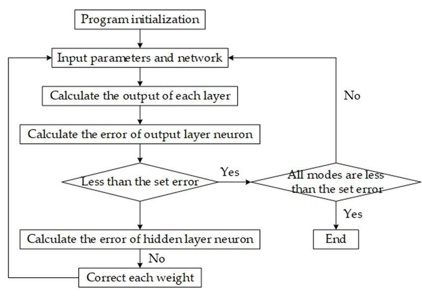
Appl. Sci. 2021, 11, 4506                                                                                                                         4 of 26

                            SU (i, j, t): cumulative spillage of car type 1 to i at review point t in the jth documented
                            circle, SU (i, j, 0) = 0;
                            IU (i, j, t): unconstrained estimation of car type i in ∆t in the jth documented circle, partic-
                            ularly IU (i, j, 0) = 0;
                            TU (i, j, t): real value of car type i in ∆t in the jth documented circle.

                            2.2. Unconstrained Estimation Methods
                                  For the revenue management system, the starting point of analysis is some set of
                            assumptions regarding an underlying stochastic or deterministic demand process [30]. In
                            fact, when the real customer demand exceeds the preset order quantity limit, the recorded
                            demand data in the presale system would be censored. Using these “cutoff demand data”
                            for demand forecasting is bound to reduce the accuracy of forecasts and directly impact
                            the revenue. Therefore, deducing the real historical customer demand from the recorded
                            demand data is the first problem. Some common unconstrained estimation methods are
                            as follows.

                            2.2.1. Expectation Maximization
                                  EM is one of the most common methods to restore incomplete data by using the
                            iterative algorithm in statistics. The EM algorithm is mainly composed of two steps,
                            E (expectation) and M (maximization)—that is, after initializing the parameters to be
                            estimated through the observable incomplete data information, the conditional expectation
                            of missing information in the incomplete data is calculated by parameter estimation, and
                            the missing information is replaced accordingly. In step E, an expected log-likelihood
                            function of complete data is obtained. In step M, the improved parameter values are
                            obtained by using this function through the maximum likelihood estimation method. The
                            whole process will be repeated until convergence [31].
                                  Considering the unconstrained demand X in ∆t with the expectation µ and variance
                            σ2 , the initial values are then
                                                                                   J
                                                                                  ∑ IB(i, j, t) I (i, j, t)
                                                                                  j =1
                                                                   µ(i, t)(0) =                                                                      (1)
                                                                                             J
                                                                                             ∑ I (i, j, t)
                                                                                          j =1

                                                                        J n                                     o2
                                                                                                 (0)
                                                                        ∑ [ IB(i, j, t) − µ(i, t) ] I (i, j, t)
                                                                        t =1
                                                   σ2 (i, t)(0) =                                                                                    (2)
                                                                                         J
                                                                                         ∑ I (i, j, t) − 1
                                                                                       t =1

                                 When all data is constrained, µ(i, t) and σ2 (i, t) cannot be initialized properly, and the
                            repairing process is abandoned. Let the unconstrained preliminary estimation value be
                            equal to the increment of the observed value; then, the unconstrained estimation value
                            after k iterations will be

                                                           IU (i, jj , t)(k) = IB(i, j, t) + IU (i, j, t)(k−1)                                       (3)

                                When only one set of data is constrained, σ2 (i, t) initialization is abandoned, and the
                            convergence is tested directly by µ(i, t). The kth iteration is divided into two steps.
                            Step E: unconstrained estimation value is
                                                                                                           R∞
                                                                                                             IU (i,j,t)(k−1)
                                                                                                                                    x f ( x )dx
                                                         (k)                                  ( k −1)
                                          IU (i, j, t)         = E[ X | X ≥ IU (i, j, t)                ] = R∞                                       (4)
                                                                                                             IU (i,j,t)   ( k −1)    f ( x )dx
Appl. Sci. 2021, 11, 4506 5 of 26
where f ( x ) is the normal probability density function, and IU (i, j, t)(0) = IB(i, j, t) when
k = 0.
Step M: find the partial derivative of the log-likelihood function Q(µ, σ2 ) versus µ(i, t)(k−1)
_ _2
and σ2 (i, t)(k−1) , and let them equal 0 to calculate the re-estimated µ and σ .
J J
2 2
∑ [ IB(i, j, t) − µ] I (i, j, t) + ∑ [ IB(i, j, t) − µ] [1 − I (i, j, t)]
J j =1 j =1
Q(µ, σ2 ) = ln L(µ, σ2 ) = − ln 2π − J ln σ − (5)
2 2σ2
( )
J J
_ 1
µ = µ(i, t) (k)
=
J ∑ IB(i, j, t) I (i, j, t) + ∑ IU (i, j, t) ( k −1)
[1 − I (i, j, t)] (6)
j =1 j =1
( )
J J
_2 1 ( k −1) 2 ( k −1) 2
2
σ = σ (i, t) (k)
=
J−1 ∑ [ IB(i, j, t) − µ(i, t) ] I (i, j, t)+ ∑ [ IU (i, j, t) ( k −1)
− µ(i, t) ] [1 − I (i, j, t)] (7)
j =1 j =1
Convergence condition: the operation should be stopped when |µ(i, t)(k) − µ(i, t)(k−1) | ≤ ε
or |σ2 (i, t)(k) − σ2 (i, t)(k−1) | ≤ ε, where ε is any small given number. Otherwise, go back to
step E and continue iterating.
2.2.2. Projection Detruncation
The initial values, convergence time, and iteration number of the EM algorithm in
the iterative process are more susceptible to their own data in varying degrees. Based
on the EM algorithm, Hopperstad proposed PD, which solves the limitation of EM in a
large-scale unconstrained estimation [32,33]. The research proves that the PD algorithm is
more flexible in practical applications.
PD and EM have the same principle, both of which include step E and M. Both
algorithms use the iterative idea of statistics to estimate the parameters of constraint
demand data, but the difference is that the parameter-related heuristic method is used in
PD at step E. In PD, the unconstrained estimation value is gained without calculating the
conditional expectation of the constraint data. In step M, the convergence conditions are
the same, namely
IU (i, j, t)(k) = E[ X | X ≥ IU (i, j, t)(k−1) ]
R∞
= IU (i,j,t)(k) f [ x |µ(i, t)(k−1) , σ2 (i, t)(k−1) ]dx (8)
R∞
= τ IB(i,j,t)(k−1) f ( x |µ(i, t)(k−1) , σ2 (i, t)(k−1) )dx
When IU (i, j, t)(k−1) > µ(i, t)(k−1) ,
v
u !#2
( k −1) ( k −1)
"
IU (i, j, t) − µ(i, t)
u
( k −1) −
IU (i, j, t)(k) = µ(i, t) + t−1.6σ2 (i, t) ( k 1 )
ln 1 − 1 − 2τ + 2τΦ (9)
u
( k −1)
σ (i, t)
When IU (i, j, t)(k−1) ≤ µ(i, t)(k−1) ,
v
u !#2
IU (i, j, t)(k−1) − µ(i, t)(k−1)
u "
( k −1) ( k −1)
IU (i, j, t)(k) = µ(i, t) 2
− t−1.6σ (i, t) ln 1 − 1 − 2τ + 2τΦ (10)
u
σ (i, t)(k−1)
where Φ( x ) is the distribution function of normal distribution, and parameter τ is any
given constant (0 ≤ τ ≤ 1) and stays the same throughout the whole process. τ repre-
sents the probability that the observed constrained demand has a true value greater than
E[ X | X ≥ IU (i, j, t)(k−1) ]. Instead of calculating a conditional expectation, in the probability
distribution graph (Figure 2), PD balances two things. The first is the area of the probabil-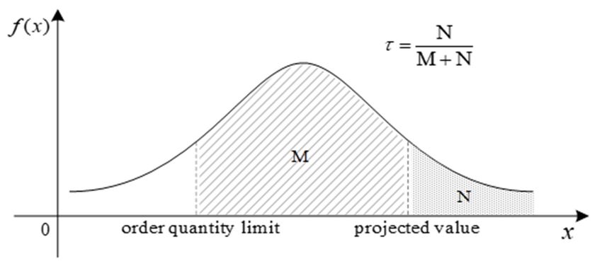
σ (i, t )
where Φ ( x ) is the distribution function of normal distribution, and parameter τ is
any given constant ( 0 ≤ τ ≤ 1 ) and stays the same throughout the whole process. τ rep-
Appl. Sci. 2021, 11, 4506 resents the probability that the observed constrained demand has a true value greater6than
of 26
E[ X | X ≥ IU (i, j, t )( k −1) ] . Instead of calculating a conditional expectation, in the prob-
ability distribution graph (Figure 2), PD balances two things. The first is the area of the
probability distribution
ity distribution betweenbetween
the order the order quantity
quantity limit (thatlimit
is,(that is, the original
the original constrained
constrained value)
value) and the new estimate or projected value (area M), and the other
and the new estimate or projected value (area M), and the other is the area between is the area between
the
the
newnew estimate
estimate andand infinity
infinity (area
(area N).N).TheThe horizontal
horizontal axisaxis value
value corresponding
corresponding to region
to region N
N represents
represents thethe portion
portion ofof thereal
the realdemand
demandthat
thatisisunderestimated
underestimatedby by the
the unconstrained
unconstrained
estimation [34]. When ττ==0.5, 0.5the
, thePD PD algorithm
algorithm cancan truly
truly balance
balance thethe values
values of and
of M M and
N,
N, yielding nearly similar results to the EM
yielding nearly similar results to the EM algorithm.algorithm.
Figure 2. Estimation process for constrained observations using PD.
2.2.3. Multitype Spill Model
2.2.3. Multitype Spill Model
The multitype spill model (MSM) takes into account the vertical recapture of different
The multitype spill model (MSM) takes into account the vertical recapture of differ-
price grade requirements, where the buyer’s behaviors of buyup and buydown indwell in
ent price grade requirements, where the buyer’s behaviors of buyup and buydown in-
different price levels. Therefore, the unconstrained estimation process based on MSM is
dwell in different price levels. Therefore, the unconstrained estimation process based on
closer to reality, which can effectively avoid the overestimation of real demand due to the
MSM is closer to reality, which can effectively avoid the overestimation of real demand
repeated records of the revenue management system’s actual observable demand between
due to the repeated records of the revenue management system’s actual observable de-
different car type prices. The spill model is mainly divided into two parts, the first part
mand between different car type prices. The spill model is mainly divided into two parts,
being the calculation of spillage, and the second part being the calculation of unconstrained
the first part being the calculation of spillage, and the second part being the calculation of
demand [35]. The specific calculation process is as follows:
unconstrained demand [35]. The specific calculation process is as follows:
1. Check if the rental demand is constrained in ∆t . When I (i, j, t) = 1, the rental demand
is not constrained and no repair is performed; otherwise, the repairing process is
performed, go to next step.
1 , C (i, j, t) − B(i, j, t) < 0
I (i, j, t) = (11)
0 , C (i, j, t) − B(i, j, t) ≥ 0
2. Parameters initialization. The distribution parameters of the demand in ∆t are initialized
by the observable “unconstrained demand”, which is the same as the EM algorithm.
3. Calculation of spillage and cumulative spillage. According to the assumptions, the
customer’s willingness to pay is characterized from low to high car type, so the
spillage should be calculated from the lowest car type.
• For a single car type, cumulative spillage can be determined by the following formula:
0 , I (1, j, t) = 1
SU (1, j, t) = R∞ (12)
c f i,t ( x )( x − c)dx , I (1, j, t) = 0
where c = IB(i, j, t), f i,t ( x ) is the probability density function of unconstrained
demand for car type i in ∆t . When I (1, j, t) = 0, rental demand was constrained,
Z ∞
SU (1, j, t) = f i,t ( x )( x − c)dx = σφ(b) + (µ − c)[1 − Φ(b)] (13)
c
c−µ
where b = σ , φ( x ) is the distribution function of standard normal distribution,
and Φ( x ) is the distribution function of standard normal distribution [36].Appl. Sci. 2021, 11, 4506 7 of 26
• For a multitype situation, when i = 1, considering cumulative spillage SU ( I, j, t − 1)
at review point t − 1 from car type 1 to I.
SU ( I, j, t − 1) , I (i, j, t) = 1
SU ( I, j, t) = R∞ (14)
c f 1,t ( x )[ x − c + SU ( I, j, t − 1)]dx , I (i, j, t) = 0
When I (i, Tj , 1) = 0,
Z ∞
SU ( I, j, t) = f 1,t ( x )[ x − c + SU ( I, j, t − 1)]dx = σφ(b) + [SU ( I, j, t − 1) − σb][1 − Φ(b)] (15)
c
When i > 1, calculate SU (i, j, t) by considering the cumulative spillage SU (i − 1, j, t)
at review point t from car type 1 to i − 1.
SU (i − 1, j, t) , I (i, j, t) = 1
SU (i, j, t) = R∞ (16)
c f i,t ( x )[ x − c + SU (i − 1, j, t)]dx , I (i, j, t) = 0
When I (i, Tj , 1) = 0,
Z ∞
SU (i, j, t) = f i,t ( x )[ x − c + SU (i − 1, j, t)]dx = σφ(b) + [SU (i − 1, j, t) − σb][1 − Φ(b)] (17)
c
4. Calculate spillage.
SU (1, j, t), i=1
U (i, j, t) = (18)
SU (i, j, t) − SU (i − 1, j, t), i>1
5. Get the repaired result, namely unconstrained estimation.
IB(i, j, t), I (i, j, t) = 1
IU (i, j, t) = (19)
IB(i, j, t) + U (i, j, t), I (i, j, t) = 0
2.3. Improved Multitype Spill Model
Generally, traditional revenue management assumes that customer selection behavior
is short sighted and ignores customer subjectivity. However, competition in the car rental
market has intensified, and the “buyer market” has gradually expanded, so the subjective
initiative of customers has been more fully reflected. The customer can choose target
commodity according to his or her own preferences and subjective utility. These factors can
be divided into three categories according to the differences in sources, namely accidental
factors, objective factors, and subjective factors.
Accidental factors are not expected and have some randomness, such as concerts,
sports events, and weather changes. Objective factors are external factors, which are
generally not changeable in a short period of time. Objective factors are not directly related
to the customers themselves, including policy and regulations, regional economic level, and
rental vehicle attributes. Subjective factors are the customer’s own determinants, which
are expressed in terms of customer preferences, trip purposes, age, and literacy. Subjective
factors can be grasped by the analysis of the customer’s choice intention, usually in the
form of a questionnaire.
2.3.1. SP/RP Survey
The basic data of customer selection preference were obtained by stated preference
(SP) and revealed preference (RP) surveys. The SP survey preresearches the subjective
preferences of customers when renting a car before the rental occurs. The RP survey
analyzes the actual selection behavior of customers in the context of what has happened.
SP data were more flexible, while RP data were more reliable.
The SP survey can obtain multiple data from a single interviewee, with the advantages
of small sample and low survey cost. The basic principle of the SP survey is to predetermineAppl. Sci. 2021, 11, 4506 8 of 26
the various attribute factors and their influence levels and then invite interviewees to score
the plan in the set situation. The respondents’ choices may be different from their actual
actions, but they can still find the main factors that can be calculated and have a large
impact on the overall mean. Then, the secondary factors that are difficult to measure will
be removed. The data obtained from the RP survey are the actual occurrence data, since
the data records behaviors that have been taken by the respondent or the actual selection
behavior observed. The basic principle of the RP survey is to describe the occurrence or
existence of the situation with different attribute factors and influence levels and to invite
the respondents to score the content.
Before the SP survey plan is designed, condition attributes, decision attributes, and
corresponding level values should be determined. The survey content includes the impor-
tance of the brand effect, the satisfaction of car rental type, the sensitivity of the rental price,
returning location, satisfaction of the vehicle status, and the satisfaction with a special offer,
service attitude, procedure convenience, and accident handling. The RP survey is aimed at
customers who have made choices, and the influencing factors are rated as very satisfied,
satisfied, general, not satisfied, and very dissatisfied. The survey includes the type of rental
vehicle and satisfaction with the rental price, return location restrictions, vehicle status,
service attitude, procedure convenience, and accident handling when the preferred rental
vehicle is rejected. See Appendices A and B for the SP/RP questionnaire of the case study.
Customers are affected by many attributes when selecting multiple models. In order
to determine the degree of influence of each attribute, AHP is usually used. AHP (analytic
hierarchy process) is an easy way to quantitatively and qualitatively deal with some fuzzy
and complex subjective problems. The most critical step is to obtain a judgment matrix
by pairwise comparison to calculate the weight of each factor. The specific calculation
process is not given. However, due to the uncertainty of expert experience, the subjective
constructed judgment matrix may not meet the conditions of complete consistency. In
order to reduce the inconsistency of subjective judgment, the VPRS (variable precision
rough set) can be used to simplify the factors affecting the customer’s choice behavior, and
similar factors are described by several factors to construct the judgment matrix.
VPRS expands the Pawlak rough set by introducing a confidence level η (0.5 < η ≤ 1),
so that admissible classification error is allowed to a certain extent. It can improve the
flexibility of decision rules and, at the same time, reflect the correlation in data analysis,
which is beneficial to the discovery of relevant data from unrelated data, that is, the implicit
patterns in the data can be more clearly expressed [37]. n o
Let S = (U, A, V, f ) be an information system, where U = u1 , u2 , · · · , u|U | is a
n o
finite nonempty set called the domain object space. A = a1 , a2 , · · · , a| A| is a finite
nonempty subset of attributes. If the attribute in A can be further divided into two disjoint
nonempty subsets, namely the conditional attribute set C 6= O and decision attribute set
D 6= O, A = C ∪ D, X ⊆ U, C ∩ D = O, then S is called the decision table. V is the union
of the attribute domains, i.e., V = ∪Va for a ∈ A, where Va denotes the domain of attribute
a; f is an information function which associates a unique value of each attribute with every
object belonging to U.
For any subset P 6= O and P ⊆ C, R( P) = {( x, y) ∈ U × U : f ( x, p) = f (y, p), ∀ p ∈ P}
is an equivalence relation on U, then the corresponding equivalence class is represented as
[ x ] p . By replacing the inclusion relation with a majority inclusion relation in the original
definition of lower approximation of a set, we obtain the following generalized notion
η-lower approximation and η-upper approximation:
[x] p ∩ X
apr η ( X ) = ∪ [ x ] p : ≥η (20)
p [x] p Appl. Sci. 2021, 11, 4506 9 of 26
η
[x] p ∩ X
apr p ( X ) = ∪ [x] p : ≥ 1−η (21)
[x] p
Then, the classification accuracy can be defined as
( )
[x] p ∩X
∪ x∈U: ≥η
[x] p
η
γ ( P, D ) = (22)
|U |
where γη ( P, D ) measures the percentage of knowledge that can be correctly classified in
the existing knowledge given a certain η in the domain.
2.3.2. Intention Analysis
Nine factors affecting the customer’s car rental behavior are regarded as conditional
attributes by the Delphi method (Table 1), and the level values of the conditional attribute
are defined by three grades: 1 = satisfaction, 2 = something in between, and 3 = dissatisfac-
tion. The level values of the decision attribute can also be defined by three grades: R = rent,
B = book but not necessarily rent, and G = give up.
Table 1. Factors affecting customer car rental choice behavior.
Factors Subjective Factors Objective Factors Random Factors
√
Company brand c1 √
Car rental type c2 √
Rental price c3 √
Special offer c4 √
Service attitude c5 √
Returning location c6 √
Vehicle status c7
Procedure √
convenience c8 √
Accident handling c9
Two rental sites (International Convention & Exhibition Center and Jiangbei Airport)
of China Auto Rental Inc. (Beijing, China) were selected in Chongqing, China. Interviewees
were randomly selected near each site, and the investigators cooperated to fill out the
questionnaire. A total of 50 questionnaires were distributed and 40 questionnaires were
returned, of which 30 were valid. By sorting out and analyzing the survey data, customer
selection decision information can be obtained, as shown in Table 2.
The following equivalence classes are available:
U/C = ( X1 , X2 , · · · , X9 ), where X1 = {u1 , u9 , u16 , u19 , u30 }, X2 = {u2 , u8 , u12 , u15 , u18 , u29 },
X3 = {u3 , u20 , u23 , u28 }, X4 = {u4 , u17 , u22 , u25 }, X5 = {u5 }, X6 = {u6 , u10 , u24 , u26 },
X7 = {u7 , u14 , u21 , u27 }, X8 = {u11 }, X9 = {u13 }.
U/D = ( DR , DB , DG ), where DR = {u3 , u7 , u8 , u11 , u12 , u14 , u20 , u21 , u23 , u27 , u28 },
DB = {u2 , u5 , u6 , u10 , u13 , u18 , u24 , u26 }, DG = {u1 , u4 , u9 , u15 , u16 , u17 , u19 , u22 , u25 , u29 , u30 }.
apr η ( DR ) = { X3 , X7 , X8 }, apr η ( DB ) = { X1 , X4 }, apr η ( DG ) = { X5 , X6 , X9 }.
p p p
Classification accuracy of VPRS is an evaluation of the ability to perform object
classification with a confidence level. Let η = 0.8. Similarly, the classification quality of
each attribute division can be determined according to Equations (20)–(22).
η η η η η
γη ( P, D ) =4/5,γc1 ( P, D ) = γc2 ( P, D ) = γc4 ( P, D ) = 0,γc3 ( P, D ) = γc5 ( P, D ) = 7/15,
η η η η
γc6 ( P, D ) = γc8 ( P, D ) = 2/15, γc7 ( P, D ) = γc9 ( P, D ) = 1/5.
The case where there is zero in the above classification quality indicates that some
interleaved repetitions or substitutions exist among the nine main attributes. Therefore,
there are six main factors affecting customer choice, namely rental price c3 , service attitudeAppl. Sci. 2021, 11, 4506 10 of 26
c5 , returning location c6 , vehicle status c7 , procedure convenience c8 , and accident handling
c9 . By comparing the six elements in pairs, the importance of each factor in the conditional
attribute on the customer decision can be obtained. The judgment matrix Λ is
1 1 7/2 7/3 7/2 7/3
1 1 7/2 7/3 7/2 7/3
2/7 2/7 1 2/3 1 2/3
Λ=
3/7 3/7 3/2 1 3/2 1
2/7 2/7 1 2/3 1 2/3
3/7 3/7 3/2 1 3/2 1
Table 2. Customer selection decision information.
Condition Attribute
Object Decision Attribute
c1 c2 c3 c4 c5 c6 c7 c8 c9
u1 3 2 1 2 1 2 2 1 2 B
u2 3 1 1 1 1 1 1 2 2 G
u3 2 1 2 2 2 2 2 1 1 R
u4 1 1 1 1 1 2 1 1 1 B
u5 1 2 2 3 2 2 3 1 3 G
u6 2 3 3 3 3 3 3 3 3 G
u7 1 3 2 3 2 1 1 1 1 R
u8 3 1 1 1 1 1 1 2 2 R
u9 3 2 1 2 1 2 2 1 2 B
u10 2 3 3 3 3 3 3 3 3 G
u11 2 2 1 1 1 2 1 1 2 R
u12 3 1 1 1 1 1 1 2 2 R
u13 3 2 3 3 3 2 3 1 3 G
u14 1 3 2 3 2 1 1 1 1 R
u15 3 1 1 1 1 1 1 2 2 B
u16 3 2 1 2 1 2 2 1 2 B
u17 1 1 1 1 1 2 1 1 1 B
u18 3 1 1 1 1 1 1 2 2 G
u19 3 2 1 2 1 2 2 1 2 B
u20 2 1 2 2 2 2 2 1 1 R
u21 1 3 2 3 2 1 1 1 1 R
u22 1 1 1 1 1 2 1 1 1 B
u23 2 1 2 2 2 2 2 1 1 R
u24 2 3 3 3 3 3 3 3 3 G
u25 1 1 1 1 1 2 1 1 1 B
u26 2 3 3 3 3 3 3 3 3 G
u27 1 3 2 3 2 1 1 1 1 R
u28 2 1 2 2 2 2 2 1 1 R
u29 3 1 1 1 1 1 1 2 2 B
u30 3 2 1 2 1 2 2 1 2 B
Obviously, the judgment matrix Λ is a positive and negative matrix, which fully
satisfies the consistency condition, and its maximum eigenvalue is πmax = 4. The corre-
sponding feature vector is ω = (0.629, 0.629, 0.180, 0.269, 0.180, 0.269)T . After normalizing,
the weight vector of Λ is ω = (0.292, 0.292, 0.083, 0.125, 0.083, 0.125)T .
2.3.3. Customer Choice Probability
The multitype spill model is based on traditional revenue management. The assump-
tion is that people in reality are irrational. When the product price is lower than the
willingness to pay, the customer will buy it immediately. Obviously, this assumption
ignores the initiative of the decision-making subject. In reality, individuals have various
cognitive deviations. If we do not proceed from the customer’s choice behavior, we cannotAppl. Sci. 2021, 11, 4506 11 of 26
find the customer’s car rental rules and the changing trend of demand, which is very
unfavorable to the car rental company’s ability to set prices and inventory in the later stage.
Therefore, in order to describe the customer’s choice behavior, the Logit model is used
to solve the above problems. The utility maximization theory is assumed, and the utility
size is used to measure the probability that a customer selects a certain type of vehicle. The
various attributes of different types constitute a comprehensive utility value. It is generally
believed that the greater the utility of a customer to select a particular type of vehicle, the
greater the probability that such a vehicle will be selected. Customers choose a variety
of types and make a choice after evaluating the utility based on various attributes. The
customer’s choice behavior can be described by a utility function Ui = vi + ξ i , where vi
and ξ i are the average utility and the random utility error, respectively, corresponding to
the customer’s selecting.
Assuming that the customer is rational, then each customer will choose the product
that will maximize utility. The probability that the customer chooses car type i is
Pi = P(vi ≥ vh , ∀h ∈ I, h 6= i ) = P(vi + ξ i ≥ vh + ξ h , ∀h ∈ I, h 6= i ) = P(vi + ξ i ≥ max (vh + ξ h )) (23)
∀h∈ I,h6=i
Assuming that ξ i are mutually independent and obey Gumbel distribution, then the
probability variable deviations of the two independent Gumbel distributions are subject to
the Gumbel distribution, which yields the general form of the multinomial logit model:
e vi
Pi = (24)
∑ e vi
i∈ I
Since the RP survey is based on actual conditions, the survey respondents are cus-
tomers who return cars to the rental sites. In the design of the questionnaire, the actual
upgrade or downgrade has been fully reflected. Therefore, the corresponding utility when
the customer’s rental car type is upgraded or downgraded is
Ui,l = 0.292c3 + 0.292c5 + 0.083c6 + 0.125c7 + 0.083c8 + 0.125c9 (25)
If the customer did not lease type i and then rented the type h, the probability of
upgrading or downgrading is
evi,h
Pi,h = (26)
I
∑ evi,l
l =0
l 6=h
where Pi,h is the preference probability of buyup or buydown with car type h when the
customer’s choice of car type i is rejected, and Pi,0 is the leaving probability when car type
i is rejected.
The improved multitype spill model (IMSM) needs to calculate the complete spillage
of all constrained data first and then calculate the demand transferring from other car types
which are constrained according to the customer preference probability. Excluding this
part is the spillage; then, the sum of cumulative order quantity and spillage will be the
unconstrained estimation.
0, I (i, j, t) = 1
CP(i, j, t) = R∞ (27)
c f i,t ( x )( x − c ) dx, I (i, j, t) = 0
Excluding the transferring is the spillage:
U (i, j, t) = CP(i, j, t) − [CP(1, j, t) P1,i + CP(2, j, t) P2,i + · · · + CP( I, j, t) PI,i ] (28)Appl. Sci. 2021, 11, 4506 12 of 26
Then, the unconstrained estimation is
IU (i, j, t) = IB(i, j, t) + U (i, j, t) (29)
3. Hybrid Forecasting
3.1. Selection of Forecast Method
For demand forecasting, there are three methods: quantitative analysis, qualitative
analysis, and decision analysis. Quantitative analysis relies on a large amount of historical
data and can be divided into time series forecasting, which uses time to organize data, and
the causal analysis method, which uses relationships to organize data. The time series
method is the most commonly used, in which the Holt–Winters model and moving average
method are representative. Time series forecasting can predict future demand, but it cannot
explain the reason. Causal analysis commonly uses regression analysis and simulation
methods. The causal analysis method uses the causal relationship between data to look for
changes and is generally used for macro prediction.
Qualitative analysis mainly relies on expert knowledge and experience to evaluate
and does not involve quantitative analysis. Delphi and judgments fall into this category.
Although this kind of method operates simply, the subjectivity is too strong and the effect
is also not favorable. The decision analysis method combines quantitative and qualitative
methods. At present, the market survey and randomness method are more commonly
used, but the research is not very mature. The quantitative analysis method is commonly
used to compare the above three methods.
The Holt–Winters model is a kind of time series forecasting model that avoids the
deficiencies of the moving average method. It uses a cubic smoothing equation to make
different data have different weights, and the predicted value is the weighted sum of the
previous data sequence. Larry Weatherford et al. deemed the availability of the basic neural
network more useful than traditional forecasting methods (moving averages, exponential
smoothing, linear regression, etc.) by comparing the mean absolute percentage error [38].
The backpropagation (BP) neural network is a widely used nonlinear forecast method
that can simulate the neural structure of the human brain and solve more complicated
problems. The BP neural network can use its own nonlinear characteristics to simulate
the development trend of the data, without requiring an assumption function. When
the prediction accuracy is reached, the future demand can be predicted according to the
learning situation. However, the BP neural network relies on the initial conditions and
is prone to fall into the local optimal solution. Therefore, the single prediction method
has inevitable defects, and the error accuracy may not reach the conditions for actual use.
This paper intends to use the hybrid forecasting to combine weights of multiple forecast
methods and improve the forecasting accuracy.
3.2. Holt–Winters Model
The Holt–Winters forecasting model is observed to outperform other techniques for
the time series, having changing seasonality, mean, and growth rate [39]. It is an adaptive
model that automatically recognizes changes in data patterns. For example, if the deviation
is caused by internal interference, it can be considered that the new observation has the
same influence as the original data, and thus gives the same weight to the data of different
periods. If the deviation is caused by external interference, then new observations and the
original data have different influences on the prediction results, and the new observations
have a higher impact on the prediction events. In order to show that the value of the data
in different periods has a different influence on the forecasting results, different weights
can be given to different periods.
The demand for car rental is a nonstationary time series with seasonal and cyclical
trends. The Holt–Winters model can perform very accurate forecasting of this regular time
series data, especially for trends and seasonal changes. It can decompose linear time series,
seasonal variations, and random variation time series and properly filter the impact ofAppl. Sci. 2021, 11, 4506 13 of 26
random fluctuations. The Holt–Winters model is an improvement and development of the
moving average method. It does not need to store much historical data but also considers
the importance of each period of data and uses all historical data.
First, smoothing equations can be obtained by iteration:
F
Ti,t = α U i,t + (1 − α)( Ti,t−1 + Si,t−1 )
i,t− L
Si,t = β( Ti,t − Ti,t−1 ) + (1 − β)Si,t−1 (30)
F
Ui,t = γ Ti,t + (1 − γ)Ui,t− L
i,t
where Ti,t is the smoothed value, Si,t is the trend value, and Fi,t is the seasonal index
of car type i at t after iterations. L is the length of the seasonal period, and α,β,γ are
smoothing coefficients.
Then, the predicted value at the future time point k is
F̂i,t+k = ( Ti,t−1 + kSi,t−1 )Ui,t− L+k (31)
where Ui,t− L+k is the seasonal index of car type i, which is one cycle ahead of t,
k ∈ {1, 2, · · · , kL}.
The way to determine the three smoothing coefficients α, β, and γ is to minimize
the error between the forecasted and actual values. In order to obtain more accurate and
objective parameters, the traditional method is the residual square sum minimum method.
Smoothing coefficients are all located in the interval (0, 1) and increase with 0.1 step
length. The squares of the prediction residuals are calculated separately and summed until
the smoothing coefficients corresponding to the sum of squares of the smallest residuals
are found.
3.3. BP Neural Network
The neural network generally includes an input layer, an output layer, and a hidden
layer. The input layer is located in the first, and no neurons are connected at the front
end. The output layer and the hidden layer are all connected with neurons, and the
weights have a one-to-one correspondence. The impact factors of output data include
input, weight, threshold, and excitation function. Because of the large number of neurons, a
large amount of information is stored, giving the neural network powerful data processing
capabilities. The neural network has the advantages of a strong parallel processing ability,
strong nonlinear processing ability, strong self-adaptation and learning ability, and strong
associative memory and fault tolerance.
The BP neural network has a simple structure, strong plasticity, clear learning steps,
and mathematical meaning. It has been proved that the BP neural network can simulate
any complex nonlinear mapping by selecting three layers. The BP neural network is a
feedforward type network that utilizes an algorithm of error back propagation. There are
only feedforward associations between neurons, and no feedback, intralayer, or interlayer
correlation. Linear sigmoid-type functions are generally used as excitation functions. Since
the excitation function is measurable everywhere, for a BP network, the divided area is
no longer a linear partition but an area composed of a nonlinear hyperplane, which is a
relatively smooth surface. Compared with linear partitioning, this classification is more
accurate and has greater fault tolerance. The learning method of the BP neural network
is to strictly adopt the gradient descent method, so that the analytical formula of weight
correction is also very clear.
3.3.1. Network Structure
A full connection is achieved between the upper and lower layers of the BP neural
network, and there is no connection among each neuron. Studies have shown that when
the output layer and input layer use a linear activation function and the hidden layer uses
the sigmoid activation function, a BP neural network with a hidden layer can map all3.3.1. Network Structure
A full connection is achieved between the upper and lower layers of the BP n
network, and there is no connection among each neuron. Studies have shown that w
Appl. Sci. 2021, 11, 4506 14 of 26
the output layer and input layer use a linear activation function and the hidden layer
the sigmoid activation function, a BP neural network with a hidden layer can ma
continuous functions. Therefore, when constructing a BP neural network model, onl
continuous functions. Therefore, when constructing a BP neural network model, only one
hidden
hiddenlayer
layeris
is generally used,
generally used, as shown
as shown in Figure
in Figure 3. 3.
Appl. Sci. 2021, 11, 4506
3.3.2. Learning Process
Figure 3. BP neural network topology.
Figure 3.The
BP neural network
learning topology.
process of the BP neural network consists of two parts: forwa
3.3.2. Learning Process
reverse propagation. When the propagation is positive, the sample is delivered
The learning process of the BP neural network consists of two parts: forward and
input layer and then processed by the hidden layer and passed to the output laye
reverse propagation. When the propagation is positive, the sample is delivered to the
value obtained
input layer by the
and then outputbylayer
processed does not
the hidden satisfy
layer the expectation,
and passed to the outputthen
layer.itIfenters th
propagation link, which uses the error back to the input layer and continuously
the value obtained by the output layer does not satisfy the expectation, then it enters
the backpropagation
the weight between link, whichduring
layers uses thethe
error back toprocess.
transfer the input layer
Afterand continuously
repeated propagation
corrects the weight between layers during the transfer process. After repeated propagation,
the error is small enough to be acceptable, the learning process then stops (shown
when the error is small enough to be acceptable, the learning process then stops (shown in
ure 4).4).
Figure
Figure 4. Flow chart of learning process.
Figure 4. Flow chart of learning process.
The specific learning steps are as follows:
Step 1The specific
Program learning steps
initialization. Select are as follows:
sigmoid as the activation function, then determine
the minimum error, learning rate, and momentum coefficient.
Step 1 Program initialization. Select sigmoid as the activation function, then
Step 2 Calculate output. Input the initial weight and calculate the output values of the
mine thelayer
hidden minimum error, layer
and the output learning rate, and
processing unit. momentum coefficient.
Step
Step 32 Calculate
Calculate output.
the error Inputerror
value. When the initial weight
is less than and calculate
the given the output
minimum error, go to value
Step 5; otherwise, go to Step 4.
hidden layer and the output layer processing unit.
Step 43 Backpropagation
Step Calculate the to adjust
errorthe weight
value. between
When hidden
error layers;
is less than then
thereuse Step
given 2.
minimum e
Step 5 Acquire the optimal output value and the weight of each layer and end the algorithm.
to Step 5; otherwise, go to Step 4.
Step 4 Backpropagation to adjust the weight between hidden layers; then reu
2.
Step 5 Acquire the optimal output value and the weight of each layer andAppl. Sci. 2021, 11, 4506 15 of 26
3.3.3. Sample Selection
After the model is established, the sample needs to be trained. In general, the training
sample needs to meet four characteristics. (1) There is a close functional relationship
between the input and object variables, and the object variable will change obviously due
to the change of input variables. (2) Input variables are independent of each other. It is
impossible to accurately calculate other components by using the components of input
variables. (3) The data to be predicted has a certain commonality with the sample data. (4)
Sample size should have a certain scale, so that the combination of all samples can reflect
the mapping relationship between output variables and target variables.
The BP neural network applies the data-driven idea, that is, using a nonlinear char-
acteristic to approximate a time series, and then using the clear logical relationship and
historical data to express future values. Suppose there is a time series { Xi }, where the
historical data is X p , X p+1 , · · · , X p+q ; to forecast the future value at time p + q + r (r > 0),
some kind of nonlinear function relationship between X p , X p+1 , · · · , X p+q and X p+q+r
needs to be found. Forecasting methods generally include single-step predictions, multi-
step predictions, and rolling predictions. Among them, the rolling prediction can reach
a certain training sample and reflects the relationship between the output sample and
predicted data. In fact, the rolling prediction starts from the single-step prediction, then
feeds the output value back to the import as part of the input for predicting future values
(see Table 3).
Table 3. Process of rolling prediction.
Step Input Output (Prediction Result)
1 X p , X p +1 , · · · , X p + q X p + q +1
2 X p +1 , X p +2 , · · · , X p + q +1 X p + q +2
.. .. ..
. . .
r X p + q −1 , X p + q , · · · , X p + q +r −1 X p + q +r
3.4. Weight Determination
Hybrid forecasting is to assign several kinds of single prediction methods to different
weights to form a comprehensive forecasting model. It can accurately and reasonably use
the valuable information of a single forecasting model, better adapt to future changes, and
reduce forecasting risk.
The key to hybrid forecasting is to properly determine the weight of various fore-
casting methods, and reasonable weights will improve the prediction accuracy greatly.
Common weight determination methods include the arithmetic average method, variance
reciprocal method, mean square reciprocal method, simple weighting method, and linear
programming method. Among them, the arithmetic averaging method is suitable for
treating each individual model equally if it is not known to each model. Usually, it is not
optimal, and the sum of squared errors is large. The variance reciprocal method, mean
square reciprocal method, and simple weighting method all have higher prediction accu-
racy than the arithmetic average method, but it is necessary to have a certain understanding
of the prediction requirements in advance. All three methods above have one thing in
common, that is, the variance is used to calculate the weight. The variance is the degree
of fluctuation of the response variable above and below the mean. When the prediction
result is not ideal and the error fluctuation is not large, the weight will still be large, which
is unreasonable.
Therefore, this paper adopts the linear programming method, which determines the
optimal weighting coefficient by taking the minimum absolute value of the combined
prediction value as the objective function.Appl. Sci. 2021, 11, 4506 16 of 26
4. Case Study and Discussion
4.1. Data Collection
This paper collected the operating data of the Huilongwan site of China Auto Rental
Inc. in Chongqing for 4 consecutive weeks (28 days). Each set of data includes the date of
pick up, vehicle brand, car rental price, and pick-up location. According to the previous
method, the model is divided into three grades according to the rental price and is set as
a “presale lead time interval” every week. The survey data is sorted out to obtain three
“presale lead time intervals” for each price grade model. The observable order quantity q
and the presale opening status of each grade model are shown in Table 4.
Appl. Sci. 2021, 11, 4506 18 of 28
Table 4. Car rental order data.
∆1 ∆2 ∆3
Variable 1 21 32 4 3 5 4 6 5 7 61 72 31 4 2 5 3 6 4 7 5 1 6 27 13 2 4 3 54 56 6 7 7
IB (1, j , t ) 11 5 75 137 313 9 3 4 9 6
IB(1, j, t) 11 43 56 3 3 9 5 12 3 5 9 1012 75 14
10 7 10 14 14
10 12 12 14 14
14
I I(1,
(1,jj,, tt)) 1 01 10 11 01 1 0 0 1 1 00 11 0 0 1 1 1 0 1 1 1 1 11 10 1 0 0 00 01 1 1 1
IBIB(2,
(2, jj,, tt)) 5 95 89 48 94 4 9 6 4 3 63 73 5 3 1 7 8 5 2 1 118 92 9
11 9 8 9 78 78 8 8 8
I (2,2, jj,, tt))
I ( 0 10 11 01 10 0 1 1 0 1 10 11 10 0 1 1 1 1 0 1 1 01 11 0 0 1 10 11 1 0 0
IBIB(3,
(3, jj,, tt)) 3 13 41 24 32 1 3 1 1 3 11 23 31 5 2 3 3 2 5 4 3 22 42 2 1 2 21 22 2 3 3
I (3,3, jj,, tt))
I (
1 0
1
1
0
1
1 1 1
1 0 1 1
0 1
0 1
1 0 1
1 1 1 1
1 1
1
1
0
1 1
0
0
1
0
1
1 1
0
0
1
1
4.2.
4.2. Applying
Applying IMSM
IMSM
According
Accordingto tothe
therental
rentalprice,
price,the
thecar
cartype
typeisisclassified
classifiedas
as11under
under$40
$40per
perday,
day,22within
within
$40–70
$40–70 per
per day,
day,andand33above
above$70
$70perperday.
day.Due
Dueto tocost
costand
andtime
timeconstraints,
constraints,aarandom
random
sampling
samplingmethod
methodwas wasused
usedto
toconduct
conductaaquestionnaire
questionnairesurvey
surveyatatsome
somerental
rentalsites
sitesof
ofChina
China
Auto Rental Inc. in Chongqing (see Figure
Auto Rental Inc. in Chongqing (see Figure 5). 5).
Figure5.5.Investigation
Figure Investigationsites
sitesof
ofChina
ChinaAuto
AutoRental
RentalInc.
Inc.in
inChongqing.
Chongqing.
The
Thesample
samplesize
sizeof
ofthis
thisRP
RPsurvey
surveywas was400,
400,and
and363
363questionnaires
questionnaireswerewerecollected,
collected,ofof
which
which320320were
werevalid
validand
and220
220of
ofwhich
whichincluded
includedbuyup
buyupororbuydown.
buydown.Discretize
Discretizethe
thesurvey
survey
data,
data,and
andlet
let“very
“verysatisfied = 10”,
satisfied “satisfied
= 10”, = 8”,
“satisfied “general
= 8”, = 5”,= “not
“general veryvery
5”, “not satisfied = 3”, =and
satisfied 3”,
and “not satisfied = 0”. The influencing factor score, utilities, and possibilities correspond-
ing to various choice behaviors can be obtained (Table 5).
Table 5. Influencing factor scores, utilities, and possibilities.
Condition AttributeYou can also read