Understanding small Chinese cities as COVID 19 hotspots with an urban epidemic hazard index - Nature
←
→
Page content transcription
If your browser does not render page correctly, please read the page content below
www.nature.com/scientificreports
OPEN Understanding small Chinese
cities as COVID‑19 hotspots
with an urban epidemic hazard
index
Tianyi Li1*, Jiawen Luo2 & Cunrui Huang3,4,5
Multiple small- to middle-scale cities, mostly located in northern China, became epidemic hotspots
during the second wave of the spread of COVID-19 in early 2021. Despite qualitative discussions
of potential social-economic causes, it remains unclear how this unordinary pattern could be
substantiated with quantitative explanations. Through the development of an urban epidemic hazard
index (EpiRank) for Chinese prefectural districts, we came up with a mathematical explanation for
this phenomenon. The index is constructed via epidemic simulations on a multi-layer transportation
network interconnecting local SEIR transmission dynamics, which characterizes intra- and inter-
city population flow with a granular mathematical description. Essentially, we argue that these
highlighted small towns possess greater epidemic hazards due to the combined effect of large local
population and small inter-city transportation. The ratio of total population to population outflow
could serve as an alternative city-specific indicator of such hazards, but its effectiveness is not as good
as EpiRank, where contributions from other cities in determining a specific city’s epidemic hazard
are captured via the network approach. Population alone and city GDP are not valid signals for this
indication. The proposed index is applicable to different epidemic settings and can be useful for the
risk assessment and response planning of urban epidemic hazards in China. The model framework is
modularized and the analysis can be extended to other nations.
Despite the nation-wide successful implementation of control measures against COVID-191,2,3, multiple small-
to middle-scale cities in China (Chinese cities could be ranked at a level basis (e.g., https://baike.baidu.com)
according to their development conditions; cities at or below the third level are normally referred to as small- to
middle-scale (or peripheral; see Model)) became epidemic hotspots during the early-2021 wave of the pandemic;
the list includes Tonghua, Songyuan, Suihua, Qiqihar, Heihe, and Xingtai etc.4,5. Unlike their nearby metropolis
(e.g., Shijiazhuang, Changchun, Harbin; Chinese provincial capitals), these small towns are largely unknown to
many Chinese before they are enlisted as “high-risk regions” after the local epidemic bursts, and it is indeed an
unexpected phenomenon that these towns are highlighted among the over 300 Chinese prefectural administra-
tions. It implies that the likelihood of epidemic hazards should be high in these regions. Many social-economic
factors may account for this fact6,7: for example, social scientists may observe that these towns are all located in
the northeast part of China, where local economies are often underdeveloped, and local residents are often more
behavioral active than they are supposed to be in face of the epidemic (e.g.,8); other conjectures may attend to the
fact that since these are neither coastal cities nor metropolitans where imported cases are more common, local
control measures and regulations are thus somewhat relaxed in these regions, which led to heedlessness of early
signals (e.g.,9,10), or that these northern regions have cold winters and also less residential housing space than
the south, hence the hazard of severe infections was harbored (e.g.,11). Although these arguments are sound, it
is desired that quantitative reasoning could be addressed to explain why these small Chinese towns stood out
as epidemic hotspots.
1
Department of Decision Sciences and Managerial Economics, CUHK Business School, Hong Kong, China. 2Institute
of Geophysics, ETH Zurich, Zurich, Switzerland. 3Department of Health Policy and Management, School of
Public Health, Sun Yat-sen University, Guangzhou, China. 4Shanghai Key Laboratory of Meteorology and Health,
Shanghai Meteorological Service, Shanghai, China. 5School of Public Health, Zhengzhou University, Zhengzhou,
China. *email: tianyi.li@cuhk.edu.hk
Scientific Reports | (2021) 11:14663 | https://doi.org/10.1038/s41598-021-94144-1 1
Vol.:(0123456789)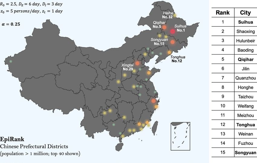
www.nature.com/scientificreports/
This points to the significant necessity of the quantification of urban regions’ epidemic hazards, desirably via
a constructed index that assesses the extent of potential risk. Such risk indices can be useful for effective deci-
sion analysis during epidemic response and planning12,13, critical to the mitigation of sudden and potentially
catastrophic impacts of infectious diseases on society14. Indeed, although the exit of COVID-19 is still on the
fly, both methodologically and practically15, it is nevertheless prudent to start getting prepared for the next
pandemic16,17,18, both economically and e cologically19,20, through comprehensive pandemic risk management
synthesis21 and the upgraded implementation of digital t echnologies22.
Many successful attempts have been made from various angles to develop such epidemic risk indices. Accord-
ing to US CDC, the preparedness for influenza pandemics can be assessed with the Influenza Risk Assessment
Tool23,24,25 through the Pandemic Severity Assessment Framework26,27; for the same purpose, the Tool for Influ-
enza Pandemic Risk A ssessment28 is recommended by WHO; and there are miscellaneous other tools developed
for national-level pandemic planning, through either mathematical simulations (e.g.,29) or scoring systems, in
which various social-economic factors are considered (e.g.,30,31,32).
However, it is suggested that currently a suitable public health evaluation framework for the assessment of
epidemic risk and response is still not full-fledge in scale33. Most proposed tools and frameworks are subject to a
number of shortcomings: (1) assessments are in most cases from the supply side (i.e., the preparedness) instead
of from the demand side (i.e., the actual risk); (2) assessments of pandemic potential are often virus-specific
(i.e., pathological), while not as general-purpose as sufficiently considering important societal factors (such as
transportation or population34); (3) many indices rely on expert scoring systems that often depend largely on
subjectivity, and the calling for mathematical models and algorithms for risk assessment and pandemic planning
is compelling35; (4) finally, many models focus on nation-wide evaluation, and there is relatively little concentra-
tion on sub-nation (e.g., city) level analysis, except for a few successful studies (e.g.,36,37,38).
To deal with these problems, in this study we develop a novel epidemic hazard index for Chinese cities,
which quantifies the potential risk of epidemic spread for Chinese prefectural administrations (over 300 units).
The index relies on a simulation model which integrates intra-city compartment dynamics with a detailed
mathematical description of inter-city multi-channel transportation. Calculation of the hazard index is based
on this dynamic system that simulates the domestic epidemic spread for user-specified diseases. In the model,
intra-city evolution is governed by the SEIR dynamics, assuming no epidemic response taken place, such that
the constructed index serves as an early-warning indicator at initial periods of epidemics, before the incidence
of any structural change in the population flow upon policy intervention (e.g.,39,40); inter-city transportation is
modeled with a multi-layer bipartite n etwork41, which makes explicit considerations of various factors during
inter-city population flow, including transit events, cross-infection due to path overlap, as well as the different
transmissivities on different transportation media.
Such a highlight on transportation (i.e., spacial patterns) is core to the city-specific risk assessment of
epidemics42 and natural hazards in general43. Indeed, over the course of the still on-going pandemic, it is acknowl-
edged that transportation, at both the global and the domestic level, plays a critical role during the spread of
viruses and to a large extent may determine the severity of the disease at different geological divisions44,45.
Essentially, compared to regression m odels46 or the machine-learning approach47, the highlight of transporta-
tion asks for epidemic risk analysis from a network perspective (e.g.,48,49,50,51), upon which the risk scores could
then be computed from quantitative a pproaches52. An important precedent is the Global Epidemic and Mobil-
ity (GLEaM) model, which integrates sociodemographic and population mobility data in a spatially structured
stochastic disease approach to simulate the spread of epidemics at the worldwide scale53. GLEaM considers
the commuting on the airport network on top of local disease transmission, where transportation is modeled
via an effective operator; our model adopts a similar methodology yet constructs a more realistic multi-layer
mathematical description of inter-city transportation, comparing also to various recent studies in the same line
of research54,55,56,57,58.
Data and methodology
Model. The base model is developed in41 and is summarized here. Assume a bi-partite graph with cities
(nodes) classified as either central cities or peripheral cities based on their development conditions (we regard
central cities as level 0-2 cities and peripheral cities as small-to-middle scale cities/towns ranking at level three
or below; see supplemental materials in41). The network is multi-layer G = (V , EA/B/R/S ), specifying four means
of inter-city transportation (thus different layers have different edge connectivites between nodes): Air (A), Bus
(B), Rail (R) and Sail (S). At each node, the local urban population is divided into four compartments: Suscep-
tible (S), Exposed (E), Infected (I), Recovered (R), and the intra-city epidemic spread follows the standard SEIR
dynamics (e.g.,59,60). We track the in- and out-flow of the exposed (E), susceptible (S) and recovered (R) popula-
tion at each node on the inter-city transportation network, which determines the open-system SEIR dynamics
(for a specific city i):
� �
Ṡi = − PSii DR0
Ii + z i + Siin − Siout
� I �
Ėi = PSii DR0
Ii + zi − DEEi + Eiin − Eiout
I (1)
E I
İi = DEi − DiI
Ṙi = DIiI + Riin − Riout .
Epidemiological parameters R0, DE , DI are the basic reproduction number, the incubation period, and the
infection period, respectively; zi = zi (t) is the zoonotic force, i.e., the seed of the disease, with zi = 0 only
at node(s) that is(are) the disease epicenter(s). The in-flow and out-flow of each city are determined via the
Scientific Reports | (2021) 11:14663 | https://doi.org/10.1038/s41598-021-94144-1 2
Vol:.(1234567890)www.nature.com/scientificreports/
q
flowmaps F q = {fi,j } between pairs of cities (i, j) specified for each means of transportation q. During inter-city
population flow, transit events are considered, where only a certain proportion of flow (the proportion is TRc/p
for central/peripheral cities, the same for each layer) enter the local population, and the rest are directed to
other destinations. Moreover, cross-infections during inter-city travels are modeled, which take place between
a susceptible person and an exposed person who share an overlapped travel path with the same destination. The
q
strength of the cross-infection spillover RT varies on different transportation media (e.g.,61).
At each city i, the exposed inflow (�Ei (t)) is given by
in
q
�Eiin (t) = fj,i (t)µj (t)(1 − TRi ),
(2)
q∈Q j∈V
where
pq (i,k)∩pq (i,j)�=0 q q q
q q
q q fj,i (1 − µj − ηj )min(dj,i , dk,i )
fj,i µj = fj,i µj + fk,i µk (RT − 1)
pq (i,k)∩pq (i,l)�=0 q q q (3)
k l fl,i (1 − µl − ηl )min(dl,i , dk,i )
q
is the adjusted exposed flow from city j to i by means q, taking care of cross-infections (di,j represents the shortest
path distance between i and j on layer q), and
q q
�Eiout (t) + fj,i (t − 1)µj (t)TRi
q∈Qj∈V
µi (t) = q , (4)
fi,j (t)
q∈Qj∈V
q q
�Riout (t) +
fj,i (t)ηj (t − 1)TRi
q∈Qj∈V
ηi (t) = q , (5)
fi,j (t)
q∈Qj∈V
are the time-stamped proportion of the exposed and recovered population among the total outflow population
from city i; thus (1 − µi − ηi ) is the proportion of the susceptible population among the total outflow from city
i. The recovered
q inf low q is tracking all the recovered people upon arrival (via ηj ):
�Riin (t) = fj,i (t)(1 − TRi )ηj (t − 1) , and according to flow balance, the susceptible inflow is
q∈Q j∈V
q q
in fj,i (t)(1 − TRi ) − �Eiin (t) − �Riin (t). The outflow population from city i’s population Pi is the
�Si (t) =
q∈Qj∈V
total outbound flow minus the transferred inbound flow, contributed by the S, E, R compartments (with the
proper assumption that I stay local, i.e., infected people do not participate in inter-city travels). Proportionally,
the outflows are:
q q q
fi,j (t) − fj,i (t)TRi
�Xiout (t) = Xi (t)
q∈Q j∈V q∈Q j∈V
. (6)
Si (t) + Ei (t) + Ri (t)
with X being S, E or R.
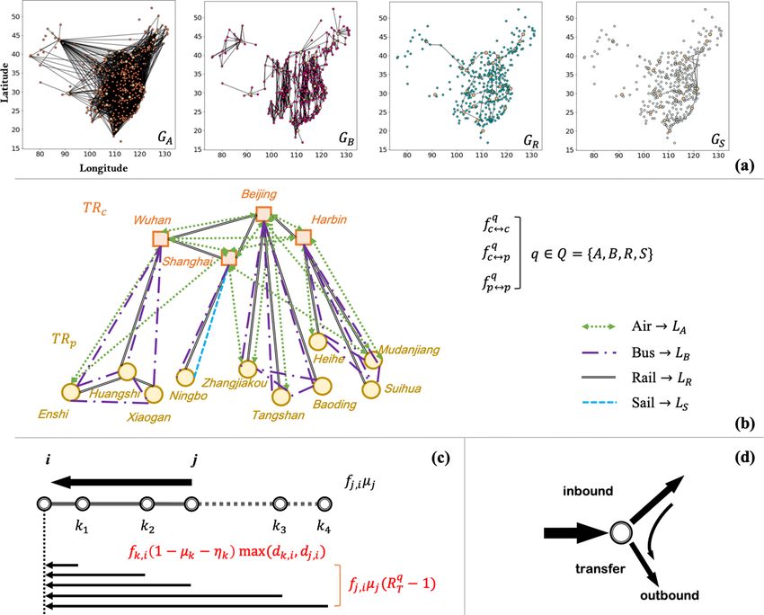
Overall, the multi-layer network model is summarized in Fig. 1 (see more details in41).
EpiRank. Using the constructed model framework, we are able to simulate the spread of imaginary diseases
of arbitrary epidemiological features, originating from arbitrary epicenters. Suppose an epidemic initiating at
node i, with a certain set of epidemiological parameters R0 , DE , DI . It is important to quantify the extent of its
propagation on the domestic scale. This calls for a specific centrality measure of the epicenter node, which can
characterize nodes’ strength in triggering epidemic spread. Borrowing from the idea of PageRank62,63, we con-
struct this new centrality score in a way similar to the eigenvalue centrality and term it as EpiRank.
Start the simulator with a disease seeded at node i upon a given zoonotic force specified with z(t), which is
non-zero during period tzs to tze . Consider a constant force z0 over such a period (whose length is tz ), and the
overall zoonotic force Z is:
tze
tze
Z= z(t)dt ∼ z(t) = (tze − tzs )z0 = �tz z0 . (7)
tzs tzs
As the simulation proceeds, the local disease spreads to the entire nation along the transportation net-
work. After τ time steps, we obtain the number of infected cases at city j, denoted as Iijτ , with the first subscript
indicating the epicenter. Similarly we obtain Rijτ , Eijτ etc. We define the normalized total infection at city j as
Uijτ = (Iijτ + Rijτ )/Z . Uijτ is then used to compute the EpiRank score for node i (denoted as hτi ):
f (Uijτ ) τ
hτi = α h + (1 − α)Uiiτ . (8)
f (Uijτ ) j
j∈G,j�=i
j∈G
Scientific Reports | (2021) 11:14663 | https://doi.org/10.1038/s41598-021-94144-1 3
Vol.:(0123456789)www.nature.com/scientificreports/
Figure 1. Multi-layer transportation network model with detailed flow description. (a) Four layers of inter-city
transportation (Air, Bus, Rail, Sail) between Chinese prefectural administrations. (b) Bi-partite categorization
of network nodes (central cities vs. peripheral cities). (c) Cross-infection during inter-city travel due to path
overlap. (d) Inbound/outbound flow during transit.
f (Uijτ ) represents a specific function of Uijτ determining the relative weights of each city j’s score contributing to
city i’s score. Here we simply allow f (Uijτ ) = Uijτ , but further considerations could be made, such as applying a
cutoff U0 and f (Uijτ ) = max(Uijτ − U0 , 0).
This score hi indicates the strength of epidemic spread at node i, which is contributed by (1) the city’s local
severity of the epidemic, and (2) its ability of spreading the disease to other cities, with the EpiRank scores of
other cities contributing to its own score at particular weights. α ∈ [0, 1] is the parameter modulating the two
effects: a small α (mode I) concerns heavier on the intra-city local spread of the epidemic ( α = 0 corresponds to
a complete local index), while a large α (mode II) puts more weight on the consequences of epicenter’s spreading
the disease to other regions.
Write W = {Wij } = {Uijτ / Uijτ }; then h = {hτi } can be calculated as follows:
j∈G
Scientific Reports | (2021) 11:14663 | https://doi.org/10.1038/s41598-021-94144-1 4
Vol:.(1234567890)www.nature.com/scientificreports/
� Uijτ
τ � τ hτj + (1 − α)Uiiτ
hi = α
Uij
j∈G,j�=i
j∈G
� Uijτ
Uτ
=⇒ (1 + α � ii )hτi = α � τ hτj + (1 − α)Uiiτ
Uijτ Uij
j∈G
j∈G
j∈G (9)
�
=⇒ (1 + αWii )hτi = α Wij hτj + (1 − α)Uiiτ
j∈G
=⇒ [I − α(W − diag(W))]h = (1 − α)diag(U )
=⇒ h = (1 − α)[I − α(W − diag(W))]−1 diag(U ) .
When α = 0, h = diag(U )1. When α = 1, h is the eigenvector of [W − diag(W)] of eigenvalue 1, in which
case we may impose a value for max(h); wlog, we consider α = 1. Note h = h(�tz , z0 ) but not h = h(Z), since
U = U (�tz , z0 ), i.e., the spread patterns may be different under different distributions of the same overall
zoonotic force.
Data and parameters. Connectivities of each network layer (i.e., transportation routes) are determined
from public datasets and empirical considerations; city information (population, GDP etc.) is obtained from
public datasets; transportation parameters (flowmap, transit rate, cross-infection strength) are determined
through fitting the early spread of COVID-19 in China during January-February 2020, where the multi-param-
eter inversion is conducted via a smart gradient method (see41 and Supplemental Materials). Transit rate at
central/peripheral cities is TRc = 0.4 and TRp = 0.05, respectively; cross-infection strength on the four trans-
portation media is {RTA , RTB , RTR , RTS } = {1.2, 3, 1.5, 1.5}; inter-city flows (elements of flowmaps) are different for
different types of city pairs (central-central, central-peripheral, peripheral-peripheral), and are determined at
A
fcc/cp/pp = 1000/500/0, fcc/cp/pp
B = 0/3000/1000, fcc/cp/pp
R = 2000/200/500, fcc/cp/pp
S = 100/100/100. These
transportation parameters well fit the early spread of COVID-19 in China (41 and Supplemental Materials) and
are fixed throughout the simulations.
For epidemiological parameters, the zoonotic force z is assumed to be 5 persons/day at Day 1 and zero after-
wards, at a single epicenter (the simulator nevertheless allows for simultaneous bursts at multiple epicenters).
The base-case disease is determined as R0 = 2.5, DE = 6 days and DI = 3 days, i.e., a mild reproduction of virus
and a medium-range infection duration, close to the clinical features of COVID or SARS (e.g.,64). Unintervened
spread of this seeded disease to all Chinese prefectural districts is simulated for 30 days, after which the ever-
infected population ( Ii + Ri ) in each city i are recorded and are used to compute the hazard index h.
Results
Cities having population larger than 1 million (300 units) participate in the calculation of h under equation (9)
(our method nevertheless applies to analysis on all >340 Chinese cities). For α = 0.25, the determined rankings
of cities’ epidemic hazards (EpiRank) are shown in Fig. 2 (top 40 shown on the graph and top 15 listed in the
table). One sees that, quite strikingly, the six small towns where the new bursts of COVID took place (Tonghua,
Songyuan, Suihua, Qiqihar, Heihe, Xingtai) are successfully highlighted by the computed hazard index. All six
cities rank within or near top 10% of all cities, including four cities ranking within top 5%. Tests suggest that the
result is robust; the high ranks of the six highlighted cities are largely invariant to fluctuations in both transporta-
tion parameters and epidemiological parameters.
The hazard rankings are computed at different α, and correlation of the ranks is demonstrated via the Spear-
man’s correlation coefficient (Fig. 3; comparing top 30 entries of each rank). A stable ranking at small values of α
is identified, along with a second invariant at the larger end (e.g., Fig. 3 top right). Indeed, the ranking is almost
completely different at, for example, α = 0.1 vs. α = 0.8, with the latter having a new set of cities ranked top in the
list, mostly located in the middle of China. This is consistent with our theory, as a small/large α points to either
of the two end-members of epidemic hazards: the intra-city local spread vs. propagating the disease to domes-
tic regions. Therefore, cities ranking high at small α (mode I) are regions with relatively large local population
(since large local population Pi substantiates large local infection Uii at city i) but also relatively small inter-city
transportation (e.g., due to their rather insignificant geological positions or modest transportation infrastruc-
tures), in which case local epidemic bursts are severely h arbored65 but not much spillovered to other cities. On
the opposite, cities ranking high at large α (mode II) are regions where inter-city transportation is sufficiently
viable (e.g., regions that are carrefours of transportation routes that have considerable access to greater domestic
population) with respect to their relatively humble local population; in this case, when seeded a virus, the epi-
center is less likely to become a closed epidemic cluster than to enormously propagate the disease to other regions.
We conducted simulations for different sets of epidemiological parameters of the assumed disease (Fig. 3),
with the combination of low/medium/high infectivity (R0 = 1.5/2.5/4) and short/medium/long infection dura-
tion ((DE , DI ) = (2, 2)/(6, 3)/(9, 10) days). The invariant at small α (mode I) is largely maintained across the
experiments, expect for a very severe disease with extremely high infectivity and extremely short duration
( R0 = 4, (DE , DI ) = (2, 2)). In this case, 30 days is sufficient for most population in most cities to get infected,
and thus top rankings lean instead on densely populated cities. The second invariant at large α (mode II) is also
identifiable, although not as clear as the first one. In some cases there is a third cluster at intermediate values of
α, but its significance is not as high as the first two. Overall, one is able to conclude that the two end-options of
EpiRank, using small or large α, lead to two converged outcomes across different scenarios of epidemic onset.
Scientific Reports | (2021) 11:14663 | https://doi.org/10.1038/s41598-021-94144-1 5
Vol.:(0123456789)www.nature.com/scientificreports/
Figure 2. Urban Epidemic Hazard Index (EpiRank) of Chinese Cities (considering cities with population
greater than 1 million; 300 units). Assuming a simulated disease with R0 = 2.5, DE = 6 days, DI = 3 days,
seeded by a 1-day zoonotic force at the strength of 5 persons/day ; α = 0.25. Table: top 15 ranks. Six hotspots
(Tonghua, Songyuan, Suihua, Qiqihar, Heihe, Xingtai) are successfully indicated by high rankings (four in top
5% and all six in top 10%). The map is generated using the python package pyecharts (http://pyecharts.herok
uapp.com).
Discussion
As mentioned, from the model and results one deduces that, the high epidemic hazard of these small towns,
obtained at low α in which case hi draws heavily on city i’s own infection Uii , derives from the combined effect
of two elements: a relatively large local population that triggers substantial local infection, and a relatively small
inter-city transportation flow determined by geological and infrastructural factors. Intuitively, a serious epidemic
cluster at the city scale is going to develop, when the city is sufficiently populated, while not much inter-city
outflow is dispersing the infection out of the epicenter. This inspires the idea that alternatively, we can compute
the population/inter-city outflow ratio of each city and use this value to indicate cities’ epidemic hazard. Results
(Fig. 4) show that similar to EpiRank, this ratio does serve as a decent hazard indicator, through which the six
epicenters are listed with high ranks. Furthermore, by contrast, shear population and annual GDP, arguably two
most considered social-economic indicators of urban regions6, are not helpful in revealing the epidemic ground-
truth. Conceptually, analysis on EpiRank help us pin down the ratio of local population/inter-city outflow as
a critical social-economic factor in explaining the observed phenomenon. For robust tests, we proportionally
increased and decreased values on the flowmaps; results suggest that the effectiveness of this ratio (and certainly
the effectiveness of EpiRank) in highlighting the six epicenters is largely invariant to changes in absolute flow
strength.
Nevertheless, it is seen that this simple ratio, although still effective and easy to compute, is not as accurate
and informative as EpiRank (Fig. 4). This time the six towns are overall lower ranked, with only 2 out of 6 in
top 5%. This is because this ratio only considers a city’s own population and transportation condition, whereas
EpiRank takes a full account of the regional and then the entire national picture, under the networked dynam-
ics approach. Indeed, it is not empirically inconsistent to argue that the six epicenters are all located in the
north, not only because they themselves have large population and small inter-city outflow, but also because it
is exactly the case that cities in northern China, with which the six towns exchange most population, all tend
to have such features and therefore the effect of local clusters is further locked in. The advantage of EpiRank is
implied; certainly, the simple ratio is also not able to reveal the extent of epicenters’ spreading the disease out,
as EpiRank can shed light on with high α.
The model framework and the EpiRank index can be used for the analysis of other nations, presumably with
a different set of transportation layers and corresponding datasets of flowmaps (e.g., for the US)54. However,
Scientific Reports | (2021) 11:14663 | https://doi.org/10.1038/s41598-021-94144-1 6
Vol:.(1234567890)www.nature.com/scientificreports/
D = 2, D = 2 D = 6, D = 3 D = 9, D = 10
E I E I E I
R = 1.5
0
0
0.1
0.2
0.3
R0 = 2.5 0.4
0.5
0.6
0.7
0.8
0.9
0 0.1 0.2 0.3 0.4 0.5 0.6 0.7 0.8 0.9
1
0.5
R = 4.0
0
0
-0.5
Figure 3. Spearman’s correlation of hazard rankings (top 30 entries in the rank) at different α (each sub-
figure), for different sets of epidemiological parameters: R0 = 1.5/2.5/4 (top to bottom) and infection duration
(DE , DI ) = (2, 2)/(6, 3)/(9, 10) days (left to right). Base case scenario (center) is R0 = 2.5 and (DE , DI ) = (6, 3).
*Suihua __
0 Zhoukou 9
Baoding 2 Yili 26
__
Hulunbeir 0 Maoming 3
*Qiqihar 1 Yongzhou 7
Shaoxing 3 Huanggang 2
Honghe 2 Dazhou 9
Jilin 1 Bijie 6
Weifang 2 *Xingtai 1
Weinan 4 Chengde 11
Taizhou 1 Hechi 6
Kashi 28 *Heihe 1
Fuzhou 2 Baicheng 13
Meizhou 2 Wenshan 8
Shantou 3 Chaoyang 12 Population/daily inter-city outflow (day)
Population (1e4 persons)
Chifeng 27 Qiandongnan 9
Annual GDP (1e8 US dollars)
*Songyuan 1 Lvliang 12
__
Quanzhou 10 Bozhou 0
Linfen 5 Linyi 14
Zunyi 3
compared with EpiRank Zhanjiang 17
__
*Tonghua 8 Liuan 0
0 500 1000 1500 2000 0 500 1000 1500 2000
Figure 4. Local population/(daily) inter-city outflow as a simplified epidemic hazard indicator (showing top 40
cities in the ranking). Compared to EpiRank (results in Fig. 2), differences are marked with green, red or black
arrows and numbers. This ratio is effective but less accurate than EpiRank in highlighting the six epicenters
(with star marks). Shear population or annual GDP does not provide similar indication.
Scientific Reports | (2021) 11:14663 | https://doi.org/10.1038/s41598-021-94144-1 7
Vol.:(0123456789)www.nature.com/scientificreports/
although providing a promising quantitative explanation for the researched phenomenon, it is indiscreet to con-
clude that EpiRank is by any means a sufficiently accurate index of urban epidemic hazards. The current dynamic
network model draws little besides the two aspects, urban population and inter-city transportation, and too many
real-world factors are left out. More importantly, a major limitation of the current analysis is that the validation of
EpiRank results is difficult to be conducted in a systematic and rigorous manner, besides using the six epicenters
as the ground truth. Indeed, the ranking is about the risk (i.e., what is likely to happen), which is not always lead-
ing to the ground truth (i.e., what did happen). Cities ranking high in the index possess great risk to be epidemic
hotspots, but the bursts may or may not turn out, and we are not able to conduct social experiments to carry out
real-world tests on this topic. Furthermore, the current assumption that infected people stay local largely holds
true in the Chinese case, but may fail in the general sense since asymptomatic people may not be diagnosed in
time and may still participate in inter-city transportation, in which case cross-infection could be more serious.
Since this factor influences all transportation flows in a proportional manner, our current normalized formula-
tion is not substantially biased; nevertheless, in future extensions, advanced SEIR compartment models could
be adopted, in which the asymptomatic stock can be separated from the infected stock, and the former group
can remain active in public transportation. Overall, despite a mathematically consistent and empirically effective
approach, the proposed simulation framework and the constructed EpiRank index call for extensive tests and
advancements in various settings, before their power as well as shortcomings can be substantially uncovered;
this study serves as a first attempt.
Conclusion
In this study, we developed an index (EpiRank) to evaluate the urban epidemic hazard of Chinese cities via
networked dynamic simulations. The index can be used in two functioning modes, and in one usage mode the
results helped provide a quantitative explanation for the phenomenon that multiple small-to-middle scale cities
in China became COVID-19 hotspots during the early-2021 wave. Through the analysis, we propose that the
combined effect of large local population and small inter-city transportation at the highlighted epicenters could
be the potential driving factor of this phenomenon. The model framework can be adapted to other nations, and
extensive assessments of EpiRank are to be conducted further.
Data availability
Edge connectivities of transportation layers and information of Chinese prefectural administrations (popula-
tion, GDP etc.) are collected from public datasets and available at https://github.com/TimothyLi0123/WH.
COVID-19 datasets used in parameter estimation are from the public repository at https://g ithub.c om/B
lanke rL/
DXY-COVID-19-Data. Scripts (python package) are available at https://github.com/TimothyLi0123/EpiRank.
Received: 27 March 2021; Accepted: 6 July 2021
References
1. Kraemer, M. U. et al. The effect of human mobility and control measures on the COVID-19 epidemic in China. Science 368(6490),
493–497 (2020).
2. Lai, S. et al. Effect of non-pharmaceutical interventions to contain COVID-19 in China. Nature 585(7825), 410–413 (2020).
3. Tian, H. et al. An investigation of transmission control measures during the first 50 days of the COVID-19 epidemic in China.
Science 368(6491), 638–642 (2020).
4. Myers, S. L. Facing New Outbreaks, China Places Over 22 Million on Lockdown (New York Times, 2021).
5. Tian, Y. L. As China COVID-19 cases rise, millions more placed under lockdown. Reuters(2021).
6. Niu, X., Yue, Y., Zhou, X. & Zhang, X. How urban factors affect the spatiotemporal distribution of infectious diseases in addition
to intercity population movement in China. ISPRS Int. J. Geo-Inf. 9(11), 615 (2020).
7. Qiu, Y., Chen, X. & Shi, W. Impacts of social and economic factors on the transmission of coronavirus disease 2019 (COVID-19)
in China. J. Popul. Econ. 33, 1127–1172 (2020).
8. Shelach, G. Leadership Strategies, Economic Activity, and Interregional Interaction: Social Complexity in Northeast China (Springer,
2006).
9. Li, A., Liu, Z., Luo, M. & Wang, Y. Human mobility restrictions and inter-provincial migration during the COVID-19 crisis in
China. Chin. Sociol. Rev. 53(1), 87–113 (2021).
10. Ye, Y., Xu, X., Wang, S., Wang, S., Xu, X., Yuan, C., Li, S., Cao, S., Chen, C., Hu, K., & Wu, X. (2020). Evaluating the control strate-
gies and measures for COVID-19 epidemic in mainland China: A city-level observational study.
11. Cao, Y., Liu, R., Qi, W. & Wen, J. Spatial heterogeneity of housing space consumption in urban China: Locals vs. inter-and intra-
provincial migrants. Sustainability 12(12), 5206 (2020).
12. Hamele, M., Neumayer, K., Sweney, J. & Poss, W. B. Always ready, always prepared? Preparing for the next pandemic. Transl.
Pediatr. 7(4), 344 (2018).
13. Morse, S. S., Mazet, J. A. & Daszak, P. Prediction and prevention of the next pandemic zoonosis. Lancet 380(9857), 1956–1965
(2012).
14. Shearer, F. M., Moss, R., McVernon, J., Ross, J. V. & McCaw, J. M. Infectious disease pandemic planning and response: Incorporat-
ing decision analysis. PLoS Med. 17(1), e1003018 (2020).
15. Thompson, R. N. et al. Key questions for modeling COVID-19 exit strategies. Proc. R. Soc. B 287(1932), 20201405 (2020).
16. Liu, W. J., Bi, Y., Wang, D. & Gao, G. F. On the centenary of the Spanish flu: Being prepared for the next pandemic. Virol. Sin. 33(6),
463–466 (2018).
17. Neumann, G. & Kawaoka, Y. Predicting the next influenza pandemics. J. Infect. Dis. 219, S14–S20 (2019).
18. Simpson, S., Kaufmann, M. C., Glozman, V. & Chakrabarti, A. Disease X: Accelerating the development of medical countermeasures
for the next pandemic. Lancet Infect. Dis. 20, e108–e115 (2020).
19. Di Marco, M. & Ferrier, S. Opinion: Sustainable development must account for pandemic risk. Proc. Natl. Acad. Sci. 117(8),
3888–3892 (2020).
20. Dobson, A. P., Pimm, S. L. & Vale, M. M. Ecology and economics for pandemic prevention. Science 369(6502), 379–381 (2020).
Scientific Reports | (2021) 11:14663 | https://doi.org/10.1038/s41598-021-94144-1 8
Vol:.(1234567890)www.nature.com/scientificreports/
21. Studzinski, N. G. & Pasteur, L. Comprehensive Pandemic Risk Management: A Systems Approach, Visiting International Research
Fellow Policy Institute (King’s College, 2020).
22. Budd, J., Miller, B. S. & McKendry, R. A. Digital technologies in the public-health response to COVID-19. Nat. Med. 26(8),
1183–1192 (2020).
23. Burke, S. A. & Trock, S. C. Use of influenza risk assessment tool for prepandemic preparedness. Emerg. Infect. Dis. 24(3), 471
(2018).
24. Cox, N. J., Trock, S. C. & Burke, S. A. Pandemic preparedness and the influenza risk assessment tool (IRAT). In Influenza Patho-
genesis and Control, Vol. I 119–136 (Springer, 2014).
25. Trock, S. C., Burke, S. A. & Cox, N. J. Development of an influenza virologic risk assessment tool. Avian Dis. 56(4s1), 1058–1061
(2012).
26. Holloway, R. et al. Updated preparedness and response framework for influenza pandemics. Morb. Mortal. Wkl. Rep. Recomm.
Rep. 63(6), 1–18 (2014).
27. Reed, C., Biggerstaff, M. & Jernigan, D. B. Novel framework for assessing epidemiologic effects of influenza epidemics and pan-
demics. Emerg. Infect. Dis. 19(1), 85 (2013).
28. World Health Organization. Tool for influenza pandemic risk assessment (TIPRA) (No. WHO/OHE/PED/GIP/2016.2). World
Health Organization (2016).
29. Eichner, M., Schwehm, M., Duerr, H. P. & Brockmann, S. O. The influenza pandemic preparedness planning tool InfluSim. BMC
Infect. Dis. 7(1), 17 (2007).
30. Grima, S. et al. A country pandemic risk exposure measurement model. Risk Manag. Healthc. Policy 13, 2067 (2020).
31. McKay, S., Boyce, M., Chu-Shin, S., Tsai, F. J. & Katz, R. An evaluation tool for national? Level pandemic influenza planning. World
Med. Health Policy 11(2), 127–133 (2019).
32. Oppenheim, B. & Ayscue, P. Assessing global preparedness for the next pandemic: Development and application of an epidemic
preparedness index. Br. Med. J. Glob. Health 4(1), e001157 (2019).
33. Warsame, A., Blanchet, K. & Checchi, F. Towards systematic evaluation of epidemic responses during humanitarian crises: A
scoping review of existing public health evaluation frameworks. BMJ Glob. Health 5(1), e002109 (2020).
34. Copiello, S. & Grillenzoni, C. The spread of 2019-nCoV in China was primarily driven by population density, Comment on
“Association between short-term exposure to air pollution and COVID-19 infection: Evidence from China’’ by Zhu et al. Sci. Total
Environ. 744, 141028 (2020).
35. Wu, J. T. & Cowling, B. J. The use of mathematical models to inform influenza pandemic preparedness and response. Exp. Biol.
Med. 236(8), 955–961 (2011).
36. Boyce, M. R. & Katz, R. Rapid urban health security assessment tool: A new resource for evaluating local-level public health
preparedness. BMJ Global Health 5(6), e002606 (2020).
37. Prieto, J., Malagón, R., Gomez, J., & León, E. Urban vulnerability assessment for pandemic surveillance. medRxiv (2020).
38. Zhu, S., Bukharin, A., Xie, L., Santillana, M., Yang, S., & Xie, Y. High-Resolution Spatio-Temporal Model for County-Level COVID-19
Activity in the US. arXiv:2009.07356 (2020).
39. Li, R. Mobility restrictions are more than transient reduction of travel activities. PNAS 118(1), e2023895118 (2021).
40. Schlosser, F. & Brockmann, D. COVID-19 lockdown induces disease-mitigating structural changes in mobility networks. PNAS
117(52), 32883–32890 (2020).
41. Li, T. Simulating the spread of epidemics in China on multi-layer transportation networks: Beyond COVID-19 in Wuhan. EPL
130(4), 48002 (2020).
42. Smith, D. L., Lucey, B., Waller, L. A., Childs, J. E. & Real, L. A. Predicting the spatial dynamics of rabies epidemics on heterogene-
ous landscapes. Proc. Natl. Acad. Sci. 99(6), 3668–3672 (2002).
43. Greiving, S., Fleischhauer, M. & Lückenkötter, J. A methodology for an integrated risk assessment of spatially relevant hazards. J.
Environ. Plan. Manag. 49(1), 1–19 (2006).
44. Christidis, P. & Christodoulou, A. The predictive capacity of air travel patterns during the global spread of the COVID-19 pandemic:
Risk, uncertainty and randomness. Int. J. Environ. Res. Public Health 17(10), 3356 (2020).
45. Liu, J., Hao, J., Sun, Y. & Shi, Z. Network analysis of population flow among major cities and its influence on COVID-19 transmis-
sion in China. Cities 112, 103138 (2021).
46. Bo, Y. C., Song, C., Wang, J. F. & Li, X. W. Using an autologistic regression model to identify spatial risk factors and spatial risk
patterns of hand, foot and mouth disease (HFMD) in Mainland China. BMC Public Health 14(1), 1–13 (2014).
47. Feng, S., Feng, Z., Ling, C., Chang, C. & Feng, Z. Prediction of the COVID-19 epidemic trends based on SEIR and AI models.
PLoS ONE 16(1), e0245101 (2021).
48. Chu, A. M., Tiwari, A. & So, M. K. Detecting early signals of COVID-19 global pandemic from network density. J. Travel Med.
27(5), taaa084 (2020).
49. Ge, J., He, D., Lin, Z., Zhu, H. & Zhuang, Z. Four-tier response system and spatial propagation of COVID-19 in China by a network
model. Math. Biosci. 330, 108484 (2020).
50. Mancastroppa, M., Burioni, R., Colizza, V. & Vezzani, A. Active and inactive quarantine in epidemic spreading on adaptive activity-
driven networks. Phys. Rev. E 102(2), 020301 (2020).
51. So, M. K., Tiwari, A., Chu, A. M., Tsang, J. T. & Chan, J. N. Visualising COVID-19 pandemic risk through network connectedness.
Int. J. Infect. Dis. 96, 558–561 (2020).
52. So, M. K., Chu, A. M., Tiwari, A., & Chan, J. N. On topological properties of COVID-19: Predicting and controling pandemic risk
with network statistics. medRxiv (2020).
53. Balcan, D. et al. Modeling the spatial spread of infectious diseases: The GLobal Epidemic and Mobility computational model. J.
Comput. Sci. 1(3), 132–145 (2010).
54. Chang, S. et al. Mobility network models of COVID-19 explain inequities and inform reopening. Nature 589(7840), 82–87 (2021).
55. Jia, J. S., Lu, X., Yuan, Y., Xu, G. & Christakis, N. A. Population flow drives spatio-temporal distribution of covid-19 in china. Nature
582(7812), 1–11 (2020).
56. Valdano, E., Okano, J. T., Colizza, V., Mitonga, H. K. & Blower, S. Using mobile phone data to reveal risk flow networks underlying
the HIV epidemic in Namibia. Nat. Commun. 12(1), 1–10 (2021).
57. Wang, B., Gou, M., Guo, Y., Tanaka, G. & Han, Y. Network structure-based interventions on spatial spread of epidemics in meta-
population networks. Phys. Rev. E 102(6), 062306 (2020).
58. Zhang, J. et al. Investigating time, strength, and duration of measures in controlling the spread of COVID-19 using a networked
meta-population model. Nonlinear Dyn. 101(3), 1789–1800 (2020).
59. Newman, M. Networks: An Introduction (Oxford University Press, 2010).
60. Sterman, J. D. Business dynamics: Systems thinking and modeling for a complex world (2000).
61. Hu, M., & Lai, S. Transmission risk of SARS-CoV-2 on airplanes and high-speed trains. medRxiv (2020).
62. Langville, A. N. & Meyer, C. D. Google’s PageRank and Beyond: The Science of Search Engine Rankings (Princeton University Press,
2011).
63. Page, L., Brin, S., Motwani, R., & Winograd, T. (1999), The PageRank citation ranking: Bringing order to the web. Stanford InfoLab.
64. Wu, J. T., Leung, K. & Leung, G. M. Nowcasting and forecasting the potential domestic and international spread of the 2019-nCoV
outbreak originating in Wuhan, China: A modelling study. Lancet 395, 689–697 (2020).
Scientific Reports | (2021) 11:14663 | https://doi.org/10.1038/s41598-021-94144-1 9
Vol.:(0123456789)www.nature.com/scientificreports/
65. Iacus, S. M. et al. Human mobility and COVID-19 initial dynamics. Nonlinear Dyn. 101(3), 1901–1919 (2020).
Acknowledgements
We thank two anonymous reviewers and the editor for many insightful comments and valuable suggestions.
Author contributions
T.L. and J.L. contribute equally to this work. C.H. helped organize, revise and review the manuscript. All authors
had read and approved the final manuscript.
Competing interests
The authors declare no competing interests.
Additional information
Supplementary Information The online version contains supplementary material available at https://doi.org/
10.1038/s41598-021-94144-1.
Correspondence and requests for materials should be addressed to T.L.
Reprints and permissions information is available at www.nature.com/reprints.
Publisher’s note Springer Nature remains neutral with regard to jurisdictional claims in published maps and
institutional affiliations.
Open Access This article is licensed under a Creative Commons Attribution 4.0 International
License, which permits use, sharing, adaptation, distribution and reproduction in any medium or
format, as long as you give appropriate credit to the original author(s) and the source, provide a link to the
Creative Commons licence, and indicate if changes were made. The images or other third party material in this
article are included in the article’s Creative Commons licence, unless indicated otherwise in a credit line to the
material. If material is not included in the article’s Creative Commons licence and your intended use is not
permitted by statutory regulation or exceeds the permitted use, you will need to obtain permission directly from
the copyright holder. To view a copy of this licence, visit http://creativecommons.org/licenses/by/4.0/.
© The Author(s) 2021
Scientific Reports | (2021) 11:14663 | https://doi.org/10.1038/s41598-021-94144-1 10
Vol:.(1234567890)You can also read