Universal power law of the gravity wave manifestation in the AIM CIPS polar mesospheric cloud images - Atmos. Chem. Phys
←
→
Page content transcription
If your browser does not render page correctly, please read the page content below
Atmos. Chem. Phys., 18, 883–899, 2018
https://doi.org/10.5194/acp-18-883-2018
© Author(s) 2018. This work is distributed under
the Creative Commons Attribution 4.0 License.

Universal power law of the gravity wave manifestation in the AIM
CIPS polar mesospheric cloud images
Pingping Rong1 , Jia Yue1,2 , James M. Russell III1 , David E. Siskind3 , and Cora E. Randall4,5
1 Center for Atmospheric Sciences, Hampton University, Hampton, VA 23668, USA
2 EarthSystem Science Interdisciplinary Center, University of Maryland, College Park, MD 20740, USA
3 Space Science Division, Naval Research Laboratory, Washington D.C., WA 20375, USA
4 Laboratory for Atmospheric and Space Physics, University of Colorado Boulder, Boulder, CO 80303, USA
5 Department of Atmospheric and Oceanic Sciences, University of Colorado Boulder, Boulder, CO 80309, USA

Correspondence: Pingping Rong (ping-ping.rong@hamptonu.edu)

Received: 4 August 2017 – Discussion started: 16 August 2017
Revised: 26 November 2017 – Accepted: 16 December 2017 – Published: 24 January 2018

Abstract. We aim to extract a universal law that governs           ground the wave signatures seem to exhibit mildly turbulent-
the gravity wave manifestation in polar mesospheric clouds         like behavior.
(PMCs). Gravity wave morphology and the clarity level of
display vary throughout the wave population manifested by
the PMC albedo data. Higher clarity refers to more distinct
exhibition of the features, which often correspond to larger       1   Introduction
variances and a better-organized nature. A gravity wave
tracking algorithm based on the continuous Morlet wavelet          Atmospheric gravity waves play important roles in atmo-
transform is applied to the PMC albedo data at 83 km alti-         spheric circulation, structure, and variability. The influence
tude taken by the Aeronomy of Ice in the Mesosphere (AIM)          of breaking gravity waves on the dynamics and chemical
Cloud Imaging and Particle Size (CIPS) instrument to ob-           composition of the 60–110 km region has been the most
tain a large ensemble of the gravity wave detections. The          significant. The momentum deposited by breaking waves
horizontal wavelengths in the range of ∼ 20–60 km are the          at mesospheric altitudes reverses the zonal winds, drives a
focus of the study. It shows that the albedo (wave) power          strong mean meridional circulation, and produces a very cold
statistically increases as the background gets brighter. We re-    polar summer mesopause region that enables polar meso-
sample the wave detections to conform to a normal distri-          spheric clouds (PMCs) to form (Fritts and Alexander, 2003;
bution to examine the wave morphology and display clarity          Garcia and Solomon, 1985). Aside from causing these in-
beyond the cloud brightness impact. Sample cases are se-           direct but fundamental effects on global circulation, gravity
lected at the two tails and the peak of the normal distribu-       waves also have widespread displays in PMCs (e.g., Fogle
tion to represent the full set of wave detections. For these       and Haurwitz, 1966; Fritts et al., 1993; Dalin et al., 2010;
cases the albedo power spectra follow exponential decay to-        Taylor et al., 2011; Thurairajah et al., 2013; Yue et al., 2014),
ward smaller scales. The high-albedo-power category has the        serving as a visible manifestation of the polar summer meso-
most rapid decay (i.e., exponent = −3.2) and corresponds to        spheric dynamics.
the most distinct wave display. The wave display becomes              Semi-organized wave-like structures have been the most
increasingly blurrier for the medium- and low-power cat-           characteristic and widespread features in PMCs. PMCs are
egories, which hold the monotonically decreasing spectral          also referred to as noctilucent clouds (NLCs) when observed
exponents of −2.9 and −2.5, respectively. The majority of          from the ground. In an extensive review given by Fogle and
waves are straight waves whose clarity levels can collapse be-     Haurwitz (1966), four types of NLCs are categorized at a
tween the different brightness levels, but in the brighter back-   descriptive level: bands and long streaks, billows, whirls,
                                                                   and veils. Most of these features resembled semi-organized

Published by Copernicus Publications on behalf of the European Geosciences Union.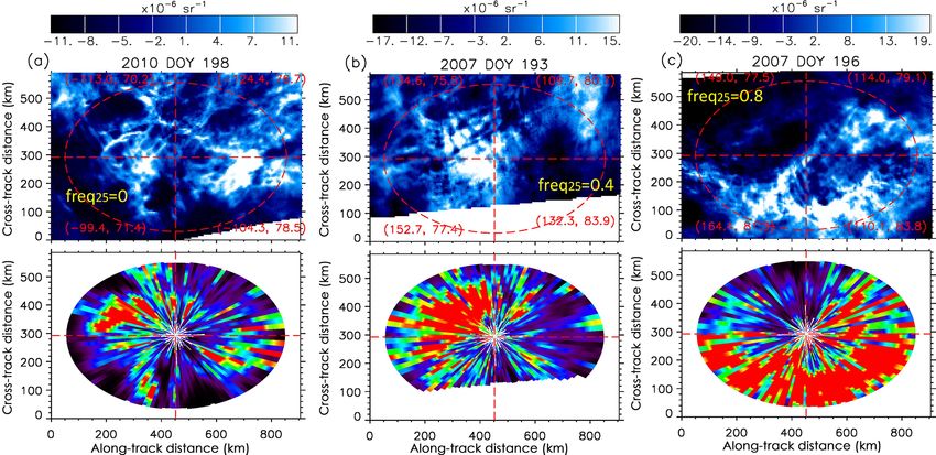
884                                                    P. Rong et al.: Universal power law of the gravity wave manifestation

wave signatures. These NLC features are reflections of grav-       play important roles in modulating the PMC spatial variabil-
ity waves, gravity wave breaking, or wave-breaking-induced         ity (e.g., Merkel et al., 2009).
turbulence (e.g., Fritts et al., 1993; Dalin et al., 2010; Baum-      In this study we developed an algorithm to quantify the oc-
garten and Fritts, 2014; Miller et al., 2015). Gravity wave        currence and manifestation of gravity waves with horizontal
horizontal scales encompass an extremely broad range of            wavelengths of ∼ 20–60 km in the CIPS Level 2 albedo data
∼ 10–1000 km (e.g., Fritts and Alexander, 2003), but the           (Lumpe et al., 2013). Such a scale range is chosen because
most widespread and readily observed displays in the NLCs          the full display of these waves can fit well into one CIPS or-
are at wavelengths shorter than 100 km (e.g., Fogle and Hau-       bital strip and also because these short-wavelength waves are
rwitz, 1966). Near-infrared hydroxyl (OH) airglow images           proven to be the most commonly observed. We aim at ob-
have also revealed similar wave patterns. For example, Tay-        taining a universal law that governs the wave display for a
lor and Edwards (1991) observed several ∼ 15–20 km wave-           large ensemble of semi-organized wave structures via sort-
length linear wave patterns over Hawaii in March, and Yue          ing their albedo disturbance power and examining their rela-
et al. (2009) reported capturing the mesospheric concentric        tionship with the background cloud brightness. The law ob-
waves with wavelengths in the range of ∼ 40–80 km over             tained will go beyond the apparent dependence of the albedo
Colorado and a few neighboring states.                             wave power on the background cloud brightness because the
   The Aeronomy of Ice in the Mesosphere (AIM) satellite           real effect of the gravity waves on the PMC brightness is
was launched in April 2007, becoming the first satellite mis-      through dynamical or microphysical control, which is related
sion dedicated to the study of PMCs (Russell III et al., 2009).    to the variability in winds, temperature, and water vapor, as is
One of the primary research goals of the AIM mission is            shown in the model studies carried out by Jensen and Thomas
to explore how PMCs form and vary. In pursuing this goal,          (1994) and Chandran et al. (2012) for instance. These stud-
gravity waves have become an increasingly important topic          ies suggested that both long and short gravity waves eventu-
in AIM science investigations. The Cloud Imaging and Parti-        ally reduce the cloud brightness locally. Generally speaking,
cle Size (CIPS) instrument (McClintock et al., 2009) aboard        the fundamental relationship between the gravity waves and
the AIM satellite provides PMC images that cover the po-           the PMC brightness is not yet fully understood. In this study
lar region daily throughout the summer season in both hemi-        we do not pursue this fundamental relationship or attempt to
spheres, and it has collected almost 10 years of data to date.     characterize specific wave events in a strict sense.
These data have enabled extensive studies of gravity wave             The algorithm we designed for CIPS differs from the wave
signatures in PMCs and of mesospheric dynamics more gen-           tracking approaches proposed in some other research papers
erally (e.g., Thurairajah et al., 2013; Yue et al., 2014). Thu-    (e.g., Chandran et al., 2010; Gong et al., 2015) in the sense
rairajah et al. (2013) presented a host of characteristic cloud    that it confines the scale range first, rather than searching for
structures in the CIPS PMC images, among which the note-           spectral peaks. This is because the wave patterns in PMCs
worthy ones include the “void” feature with a clean edge           can be obscured by larger-scale variability that possesses
and a core region of sharply reduced cloud brightness, and         larger amplitudes and also because these patterns are rarely
concentric waves (see also Taylor et al., 2011; Yue et al.,        monochromatic. As a result, spectral peaks, for example in
2014). These are fairly unique signatures with low occur-          wave numbers, do not stand out easily unless a distinct wave
rence frequency and are not the focus of the current study,        structure is first visually detected and then a spectral analy-
although we do also discuss some examples of the concen-           sis is carried out along its most optimum orientation. Such
tric waves in a later part of this paper. Yue et al. (2014) cor-   a challenge is also reflected in the airglow image process-
related concentric wave patterns in the CIPS PMC data with         ing that aims at identifying the mesospheric gravity waves
similar patterns in the stratosphere observed by the Atmo-         (e.g., Matsuda et al., 2014). In addition, it is worth mention-
spheric Infrared Sounder (AIRS) instrument aboard NASA’s           ing that in the current study we did not adopt high-pass fil-
Aqua satellite (Aumann et al., 2003). Concentric waves are         tering to extract the small-scale structures (e.g., Chandran et
the most evident proof that gravity waves excited by tropo-        al., 2010) because 2-dimensional (2-D) filtering is prone to
spheric storm systems have propagated into the mesosphere.         inducing notable artificial features if large and small scales
   Quantitatively characterizing gravity waves in PMC im-          are not separated optimally. Another important technique to
ages is generally difficult because the wave patterns are com-     detect gravity waves and to resolve their characteristics is ap-
plex, although several NLC morphology types have been              plying a spatiotemporal analysis to either the ground-based
successfully interpreted in previous modeling studies (e.g.,       or satellite measurements (e.g., Wachter et al., 2015; Ern et
Fritts et al., 1993; Baumgarten and Fritts, 2014). In addi-        al., 2011). For example, Wachter et al. (2015) applied such a
tion, PMCs are characterized by a hierarchy of larger-scale        technique to the OH airglow time series measured at the cho-
features (∼ 100–1000 km) that often obscure the smaller-           sen triangular equilateral ground sites to yield a consistent set
scale (< 100 km) gravity wave signatures. It is worth noting       of wave parameters. In these analyses, however, a full display
that these large-scale features may not be exclusively grav-       of the waves is not captured because only a few locations are
ity wave structures because tides and planetary waves also         used. CIPS, on the other hand, has extended spatial coverage,

Atmos. Chem. Phys., 18, 883–899, 2018                                                 www.atmos-chem-phys.net/18/883/2018/
P. Rong et al.: Universal power law of the gravity wave manifestation                                                          885

and therefore in the current study we aim to only detect the       resolution. In the Level 2 processing the cloud scattering sig-
spatial wave patterns.                                             nal is further distinguished from the background Rayleigh
   The structure of the paper is as follows. A brief description   signal based on their different scattering angle dependence.
of the CIPS data is given in Sect. 2. In Sect. 3 we describe       The Level 2 retrieval is operated on the Level 1b data, so that
the wave tracking approach, provide an analytical demonstra-       the Level 2 data product is registered on the same 25 km2
tion, and then apply the algorithm to a few concentric wave        resolution grids. Throughout the 10 years of the AIM mis-
patterns found in the CIPS imagery. In Sect. 4 the statistics      sion, the CIPS retrieval has experienced earlier versions, and
of the wave power are obtained, and their dependence on the        the theoretical framework of these retrievals was described
background cloud brightness is quantified. A resampling pro-       in Bailey et al. (2009). In the previous CIPS data versions
cess is applied to reach a normal distribution of all the wave     the Rayleigh background was retrieved pixel by pixel rather
power values. Resampling serves as the first step to further       than over the entire orbital strip like in version 4.20. This
examine the gravity wave display beyond the apparent im-           earlier approach will result in increased retrieval noise in the
pact of the cloud brightness. In Sect. 5 representative cases      cloud parameters, requiring additional smoothing procedure
are chosen to extract a universal law that controls the wave       to increase the signal-to-noise ratio at the expense of retrieval
display. As a step further, demonstrations of these cases are      resolution.
shown for verification. Conclusions are given in Sect. 6.

                                                                   3     Wave tracking algorithm
2   CIPS dataset
                                                                   3.1    Analytical demonstration
CIPS version 4.20 Level 2 orbital strips of PMC albedo at          One-dimensional (1-D) continuous wavelet transform
83 km altitude are used in this study (Lumpe et al., 2013).        (CWT) calculations constitute the basic elements of the
CIPS is one of the two instruments that are currently oper-        proposed CIPS wave tracking algorithm. The term “wave
ating aboard the AIM satellite. The CIPS instrument (Mc-           tracking” in the context of this paper refers to the operation
Clintock et al., 2009) is a panoramic imager viewing nadir         of tracking all existing quasi-periodic wave displays in the
and off-nadir directions to measure ultraviolet radiation (cen-    CIPS PMCs over the scale range of ∼ 20–60 km, rather
tered at 265 nm) scattered by the clouds and atmosphere. In        than tracking a specific wave event. We first demonstrate
the spectral region near 260 nm, absorption of ozone in the        the effectiveness of the approach using an analytically
lower atmosphere renders the earth nearly dark, maximizing         composed series. When the algorithm is applied to CIPS
the contrast of PMC scattering relative to the atmospheric         (see Sect. 3.2 and later), each individual CWT calculation
background. It is worth mentioning that, aside from the PMC        will be carried out along a presumably ∼ 400 km (or 80
data used in this study, the CIPS Rayleigh albedo anomaly          grids) long CIPS PMC albedo segment and will deliver
(RAA) data are also made available to the public. The RAA          a total of 22 components spanning the scales 2.0–76.0 in
data characterize the gravity waves at altitudes of 50–55 km       grids (5 km per grid). The relevant scale range for this study
(Randall et al., 2017), serving as the only existing imaging       is ∼ 4.0–12.0 grids (∼ 20–60 km), and the total power of
dataset that can reveal the gravity wave horizontal structures     the relevant CWT components is termed “CWT power” or
near the stratopause. CIPS consists of four wide-angle cam-        “albedo power” in the following CIPS-related discussion.
eras arranged in a “bowtie” shape that covers a 120◦ (along        It is worth pointing out that a ∼ 20–60 km scale range is
orbit track) × 80◦ (cross orbit track) field of view (FOV). It     focused on in this study because the total albedo power spa-
measures scattered radiances from PMCs near 83 km altitude         tial distribution corresponds well with the readily observed
to eventually derive cloud morphology and particle size in-        wave signatures in the albedo maps (see Figs. 2, 7–9, and
formation. Each individual cloud had a stack of maximum            11). The 60 km threshold appears particular, but it is chosen
seven exposures from different view angles, from which we          simply because it is among the sequence of individual scales
derive PMC scattering phase functions and eventually re-           for the CWT calculations, which are 4.0, 4.7, 5.6, 6.7, 9.5,
trieve the nadir horizontal spatial features. CIPS horizontal      and 11.3 grid units. A radius of roughly ∼ 400 km is chosen
resolution is approximately 2–7 km depending on how far a          because it is able to include many repeats (∼ 10) of the wave
given pixel is from the center of the bowtie, with the center of   ridge and trough to provide the full extent of wave display.
the bowtie possessing the finest resolution. CIPS version 4.20     Yet the spatial span of the wave display should not be overly
retrieval algorithms and data products are described in detail     extended because we do not wish to go across several wave
by Lumpe et al. (2013). In Level 1a the camera flat-fielding       events or different types of variability along the path of
is applied to remove the pixel-to-pixel variation induced by       CWT calculation. These calculations will be carried out in
each camera, and then normalization between the cameras            all 360◦ radial directions (3◦ increment) when being applied
is applied. In Level 1b all cameras are merged to create a         to CIPS PMCs.
consistent set of CIPS measurements. In this stage the mea-
surements are adjusted onto a common grid system of 25 km2

www.atmos-chem-phys.net/18/883/2018/                                                   Atmos. Chem. Phys., 18, 883–899, 2018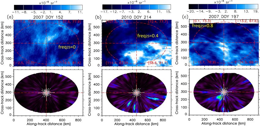
886 P. Rong et al.: Universal power law of the gravity wave manifestation
tial phases at the start point of the series. These wavelengths
are the 5th–11th scales delivered in a CWT calculation men-
tioned above. The shortest and longest of these plane waves
are shown by the gray and green dashed lines in Fig. 1a. The
total CWT power over the scales of 4.0–12.0 grids is shown
as the black curve in Fig. 1b, whereas the thick red curve in
Fig. 1b is the reconstructed series using the Morlet wavelets
and the corresponding CWT coefficients. It is notable that
the black curve is smooth and exactly follows the magnitude
change of the localized shorter scale signals. The basis vec-
tors of CWT are not orthogonal, and therefore a reverse CWT
does not exist in a strict sense, but we do find that the recon-
structed series greatly resemble the original series although
their magnitudes slightly differ. This suggests that the CWT
and reverse CWT work efficiently on a quasi-periodic signal
series. Especially, the fact that CWT almost precisely cap-
tures the local variability of the wave amplitude suggests that
the CWT algorithm will be an effective approach to detecting
the gravity waves in the CIPS PMCs.
Figure 1c shows the CWT spectrum of the created se-
ries. We just mentioned that the created series is the sum
of only seven FFT components, but since FFT and CWT
have different basis vectors, the CWT will project onto all the
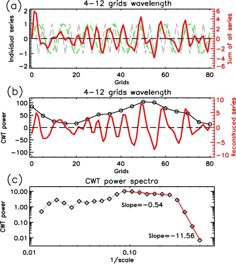
Figure 1. Demonstration of the continuous wavelet transform scales from 2.0 to 76.0 grids. Over the seven relevant scales
(CWT) applied to an artificially created series. (a) The created se- from 4.0 grids to 12 grids the slope on the double-logarithm
ries (red line) consisting of seven sinusoidal components with wave- diagram is as weak as −0.54, reflecting the fact that we
lengths (or scales) of 4.0, 4.7, 5.6, 6.7, 9.5, and 11.3 grid units, each have adopted identical amplitudes for all the plane sinusoidal
of them with the same amplitude of 1.0. The gray and green dashed waves used to create the series. For scales < 4.0 grids there
lines are for the scales of 4.0 and 11.3 grids, respectively, serving to
is an extremely rapid decrease of the CWT power density
demonstrate the individual series. Note that the red curve has used
the scale on the right axis which corresponds to a 3-times-larger
with a slope of −12, indicating that these scales are almost
magnitude. (b) The total CWT power series (black with circles) and non-existent. It is noteworthy that the created signal exhibits
the reconstructed series (red line) using the wavelet coefficients and a quasi-periodic nature even though there are no spectral
components. (c) The CWT power spectra. The slopes (i.e., red lines) peaks. However, due to the involvement of multiple scales,
are calculated over the seven scales used to create the series and the the fluctuation washes out in a certain portion of the series
smaller scales that are present due to the non-orthogonal basis in the (i.e., in the range of 3.0–23.0). In this latter case, quasi-
CWT calculation. periodicity is impaired by the involvement of multiple com-
ponents.
A 6th-order Morlet wavelet is adopted in this study. A 3.2 Demonstrations using concentric wave patterns
Morlet wavelet (Gabor, 1946) is a complex exponential
(plane sinusoidal waves) windowed by Gaussian function so In terms of applying the algorithm to the PMC images from
that both periodicity and localization can be realized, defined CIPS, a direct 2-D CWT routine would be preferred but does
2 2
as eikx/s e−x /(2s ) , where k is the (non-dimensional) order not exist in the standard numerical recipe. In addition, there
and s is the scale. Scale s determines both the width of the is ambiguity in determining the phases in the CWT algorithm
Gaussian function and the period of the sinusoidal signal. In because there is always a tradeoff between the localization of
a 6th-order Morlet wavelet (k = 6) the scale s is almost pre- the signal and a clear phase determination.
cisely the period of the sinusoidal signal. We emphasize here In this study we used an algorithm based on consideration
that in the following main analysis applied to the CIPS PMC of expediency as well as efficiency. The 1-D CWT calcula-
images the scales of the wave structures refer to the Morlet tions are carried out in all 360◦ radial directions (3◦ incre-
wavelet scales. However, we will first use an artificially cre- ment) centered at a given location within the CIPS albedo
ated series to demonstrate that CWT and fast Fourier trans- orbital strip. The resampling of the CIPS data is performed
form (FFT) deliver qualitatively consistent results. in the radial and angular directions centered at such a loca-
The artificially created series, which is shown as the thick tion. In the radial direction the increment step is 5 km, which
red curve in Fig. 1a, is composed of seven plane sinusoidal is the same as the CIPS Level 2 resolution, while in the angu-
waves that have wavelengths of 4.0 to 12.0 grids and zero ini- lar direction a step of 3◦ is chosen based on the consideration
Atmos. Chem. Phys., 18, 883–899, 2018 www.atmos-chem-phys.net/18/883/2018/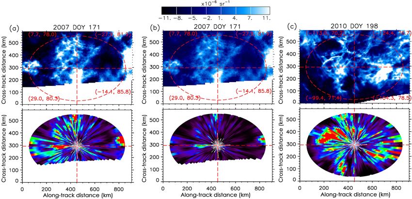
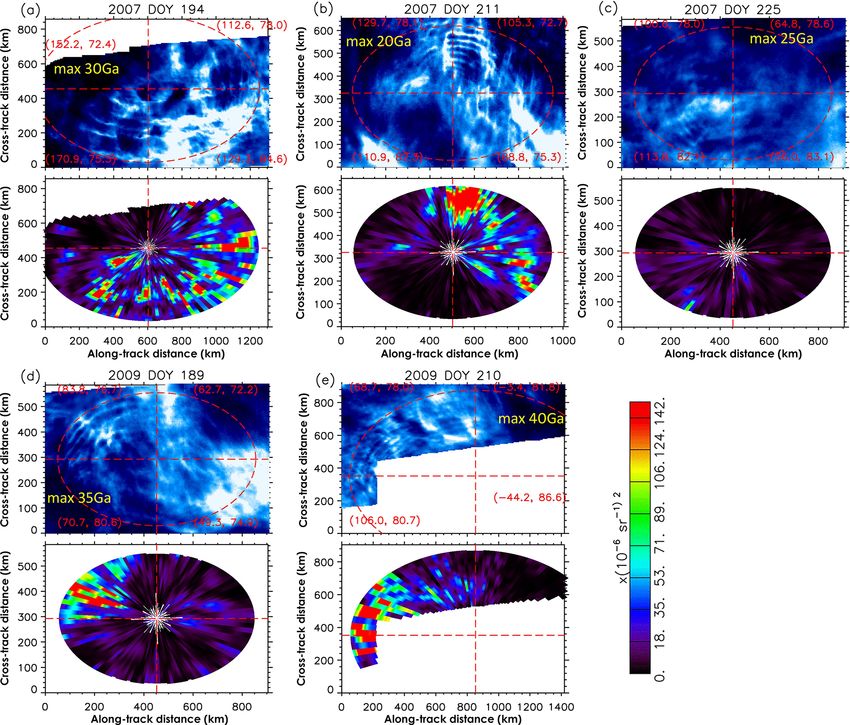
P. Rong et al.: Universal power law of the gravity wave manifestation                                                        887

of yielding a sufficiently detailed yet smooth spatial map of      the concentric waves will likely be substantially elongated
the albedo wavelet power. This approach was inspired by the        compared to those in winter or spring.
intent of detecting ideal concentric waves because such a de-         The example shown in Fig. 2a has a wavelength of about
sign will result in the maximum CWT albedo power within            60–80 km, which is longer than most other concentric waves
a given radius. In addition, performing the CWT in all radial      in the CIPS PMCs, but since the (bright) ridges are much nar-
directions will efficiently capture the waves of all orienta-      rower than the (dim) troughs the albedo power still reaches
tions. Since the basis vectors of 2-D FFT are straight (linear)    notable magnitudes. Remember that in this study only the
waves of all orientations, the current algorithm is more or        CWT power within the wavelength range of ∼ 20–60 km is
less a short version of the 2-D FFT in a localized area but        calculated, and what is shown in Fig. 2a again reminds us
has the merit of being straightforward in reflecting the local     that wave patterns in PMCs only achieve quasi-periodicity.
albedo wave power.                                                 The example in Fig. 2b is a set of highly distinct concentric
   The specifics of the algorithm are described as follows. An     waves. The albedo power reaches notably larger values when
elliptical region of 80 grids along-track and 80 × 0.65 grids      the waves are the most distinct in the upper-right quadrant
cross-track is used to carry out the CWT calculations. The         of the albedo map (see Fig. 2b, upper panel). In the upper-
factor 0.65 is empirically chosen based on a few fitted exam-      left quadrant of the albedo map the waves become blurry,
ples of the concentric waves found in CIPS. The rationale of       but one can still tell that they are concentric. In the blurry
such a factor will be revisited in a following paragraph. Con-     part of the map the albedo power decreases sharply, as is
centric waves found in CIPS appeared to be mostly elongated        clearly seen from the corresponding lower panel. Given the
in the along-track direction. This factor has no qualitative ef-   confined scale range of ∼ 20–60 km, being visually blurry
fect on the results except that, when the elliptical region fits   can be interpreted as possessing a lower variance level, which
an actually existing concentric wave pattern, it achieves the      may have been a result of diffusive processes. In the spectral
largest albedo CWT power, which is a desired condition for         space, if the leading scales stand out poorly from the neigh-
the wave tracking operation. The elliptical region is moved        boring smaller scales, then the structure will be less orga-
around to fully cover the orbital strips. The steps of the move-   nized, which also makes it less distinct. This topic will be
ment are the half axial lengths in both along-orbit and cross-     further addressed in Sect. 5. Within the same wave display,
track directions. Except for the intent to achieve full cov-       varying from being distinct to blurry must be controlled by
erage of the orbital strip, the “move-around” scheme will          some physical process yet to be unraveled. In the lower-right
also ensure the capture of the albedo CWT power from vary-         quadrant of the albedo map there are some straight waves
ing orientations in the same region. The albedo CWT power          that have cross-interfered with each other but are much less
map enclosed in the given elliptical region measures the total     distinct than the main part of the concentric waves. This sug-
albedo fluctuation intensity in the scale range of ∼ 20–60 km      gests that multiple wave packets of different morphology of-
for each spatial location.                                         ten coexist right next to each other in the PMCs. Figure 2c
   Five examples of concentric waves and the corresponding         shows an example of extremely faint concentric waves which
albedo power maps are presented in Fig. 2 to demonstrate           are characterized by much lower albedo power than those in
how the wave tracking algorithm works for CIPS. Concen-            the rest of the examples. Figure 2d shows a slightly weaker
tric waves are chosen because they are well documented as          but also fairly distinct partial concentric wave pattern that
possessing a unique morphology and meanwhile serving as a          also coexists with some blurry straight-wave patterns. Fig-
proof of the connection between the lower and higher atmo-         ure 2e is an example of concentric waves in a brighter back-
sphere. These waves are extremely rare and were detected           ground that occurred in 2009. In 2009 CIPS orbits appear
only a few times for a given PMC season. The percentage            twisted due to the camera’s turned position.
of detection is less than 5 % in terms of days per season, and        Lastly, we must also point out an inherent drawback of the
by spatial coverage the fraction is even smaller. All examples     CWT wave tracking algorithm. It is apparent that in all the
have shown only partial rings. The model results by Vadas et       examples shown in Fig. 2 the clouds (e.g., > 5.0×10⁻⁶ sr−1 )
al. (2009) simulating the concentric rings to compare with the     do not fill up the entire elliptical region, and furthermore
observations near Fort Collins, Colorado, have shown that          the wave signatures are mostly partial rings. If such an in-
including realistic zonal winds can substantially disrupt the      homogeneity is strong, the mean albedo power or back-
completeness of rings in the mesosphere, with about 50 % of        ground brightness can misrepresent the characteristics of the
the wave structure being disrupted. In the CIPS PMCs the           region. We therefore have chosen a relatively small radius
rings are more severely disrupted. In some cases only a 20◦        (∼ 400 km) to carry out the calculations to minimize the ef-
section of the full 360◦ circle has survived (not shown). The      fect of inhomogeneity. Due to the high complexity of the
model results by Vadas et al. (2009) also indicate that if a       PMC signatures, it is unlikely to simply eliminate such an
July zonal wind is adopted in the simulation the rings will be     effect. Nevertheless, so far we have not run into any note-
elongated to an axial ratio of about 0.6–0.7, which roughly        worthy problem due to such effect when analyzing the wave
agrees with the findings in CIPS. It appears that in summer        tracking results.

www.atmos-chem-phys.net/18/883/2018/                                                  Atmos. Chem. Phys., 18, 883–899, 2018
888 P. Rong et al.: Universal power law of the gravity wave manifestation
Figure 2. Wave tracking algorithm applied to the concentric waves (a)–(e) in the CIPS orbital strips. Wave tracking is carried out within
the elliptical regions. For each pair, the upper panel is the albedo, and the lower panel is the albedo CWT wave power field by 3◦ angular
bin × 5 km radial bin. Blue–white color scheme is used for the albedo maps, with the white color representing the maximum albedo values
indicated by the yellow legends, with 1 Ga = 1.0 × 10⁻⁶ sr−1 . The red numbers at the four corners are longitudes and latitudes. The rainbow
color bar for the CWT power is used universally in this paper.
4 Statistics of the gravity wave albedo power values cloud presence frequency (denoted by freq25 hereinafter) is
a better index than the mean cloud albedo in characterizing a
4.1 Brighter PMC background threshold systematically brighter cloud background.
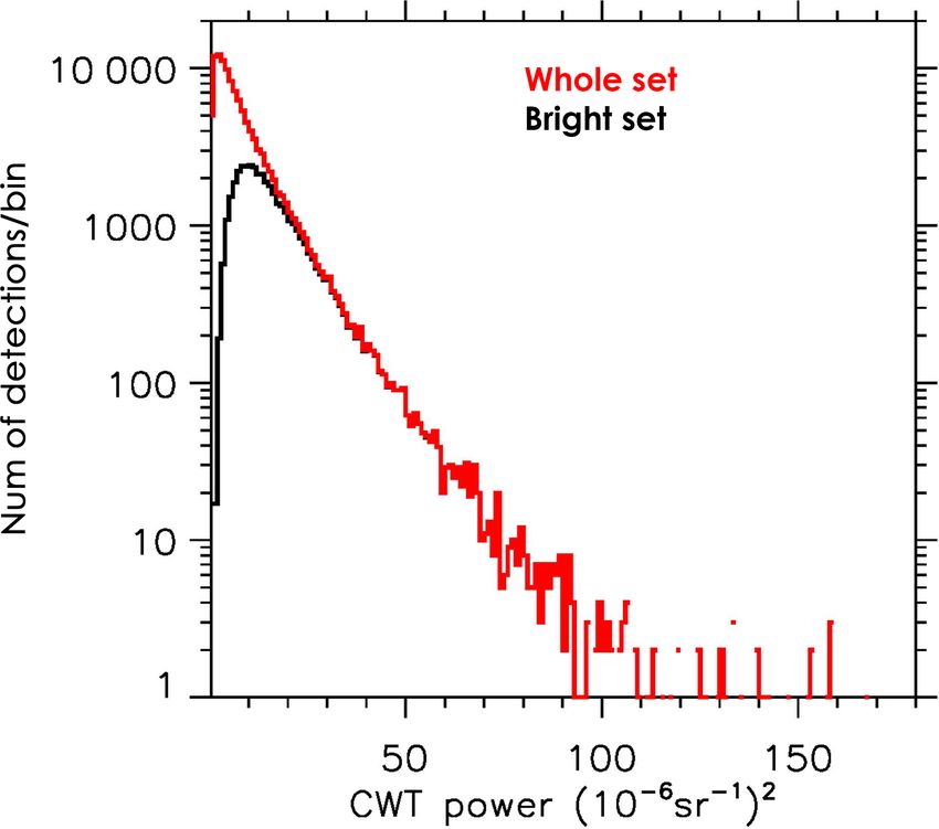
The statistical ensemble consists of the albedo power values 4.2 Histograms of the albedo power values
averaged within all elliptical regions used to carry out the
wave tracking. We need to emphasize here that the albedo Figure 3 shows the histograms of the albedo power values
power refers to the total power within the scale range of for the full set of wave detections (in red) and those residing
∼ 20–60 km. The wave tracking procedure has been carried in the brighter background (in black), and both show a peak
out throughout the two northern hemispheric summers in number density being close to zero and then a rapid decrease
2007 and 2010 from 1 June to 31 August. We take a particu- as the albedo power increases. Peak locations approaching
lar interest in the wave display in the brighter PMCs because zero indicate that the majority of the waves are in the range
the previously identified waves mostly reside in the relatively of low albedo power. It is especially worth noting that the full
dim cloud environment. We split the cloud population into set and the brighter set collapse as the albedo power is greater
two subsets, one containing only 0–2 % bright clouds (with a than ∼ 20 × 10−12 sr−2 , whereas before this point they sep-
threshold of 25 × 10−6 sr−1 ) in the elliptical region, which is arate substantially. This indicates that brighter clouds mostly
the overall dimmer cloud group, and the remaining set con- coincide with the higher albedo power and that the waves
taining a systematically larger fraction of bright clouds. The that have caused the difference in the two curves reside in the
25 × 10−6 sr−1 threshold is chosen empirically. The bright- dimmer group. In addition, the collapsing part of the curves
Atmos. Chem. Phys., 18, 883–899, 2018 www.atmos-chem-phys.net/18/883/2018/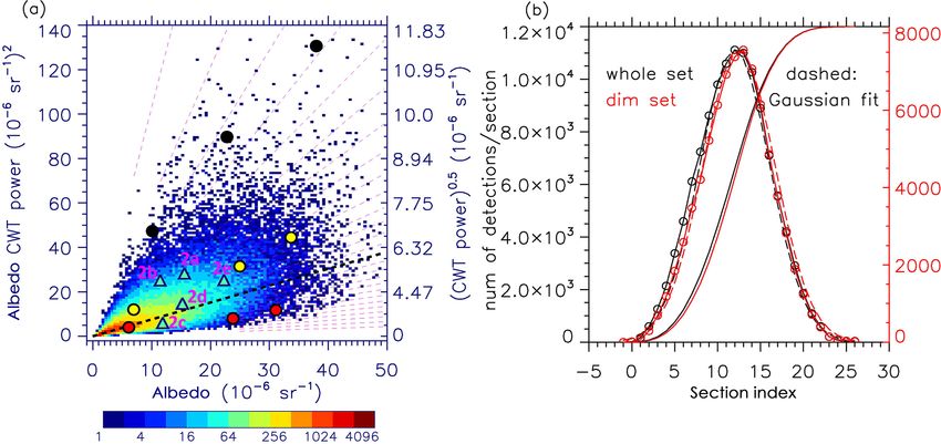
P. Rong et al.: Universal power law of the gravity wave manifestation                                                                 889

                                                                          4.3   Relationship between the albedo power and freq25

                                                                          Although the dimmer subset takes up a major fraction of the
                                                                          cloud population, which exceeds 65 %, we take just as much
                                                                          interest in the wave display in the brighter cloud background
                                                                          in this study. Figure 4 shows the scatterplot of the wave de-
                                                                          tections in the brighter cloud background on the plane of
                                                                          albedo power versus freq25 . In Fig. 4a, within equally spaced
                                                                          bins of freq25 and the albedo power, the rainbow-colored
                                                                          squares represent the number density of the wave detections.
                                                                          The dimmer group of PMCs are collapsed into the first bin of
                                                                          freq25 = 0–0.02 and is not shown in this scatterplot to avoid
                                                                          any discontinuity induced by the artificially chosen threshold
                                                                          (i.e., 25 × 10−6 sr−1 ).
                                                                             Figure 4a shows that the wave detections (see rainbow col-
                                                                          ors) are grouped more densely in the low-albedo-power as
                                                                          well as the low-brightness region. This generally agrees with
Figure 3. The histograms of the CWT power values obtained                 what Fig. 3 shows, but we should note that the wording “low”
throughout the two northern hemispheric summers in 2007 and
                                                                          is in a relative sense because we have taken away the dimmer
2010. Each CWT power value refers to an average within a given
                                                                          set in this analysis. For any given freq25 the wave detection
elliptical region. The black curve is for the brighter cloud group that
corresponds to freq25 > 2 % within a given elliptical region, and the     number density distribution resembles a normal distribution,
red curve is for the full set of detections. The bin size within which    but the outliers are strongly asymmetric, showing a much-
we count the detection number is 1.0 × 10⁻¹² sr−2 .                       further-reaching albedo power value at the upper limits. In
                                                                          addition, we find that as freq25 increases the peak number
                                                                          density moves toward an increasingly larger albedo power,
forms a straight line under a logarithmic vertical axis, sug-             shown by the dashed black curve. Both suggest that in a
gesting an exponential decrease of the wave detection num-                statistical sense larger albedo power corresponds to brighter
ber density as the albedo power exceeds the value where the               cloud background. At the dimmer end where freq25 = 0.02
peak number density occurs. For the full set of the wave de-              the albedo power is within 50 × 10−12 sr−2 (amplitude ∼
tections the straight line proceeds to a much smaller albedo              7.0 × 10⁻⁶ sr−1 ), while for freq25 = 1.0 it reaches values
power value, while for the brighter set it shows a peak at a              greater than 150×10−12 sr−2 (corresponding to an amplitude
higher albedo power. Removal of the dimmer cloud group by                 of ∼ 12.0 × 10⁻⁶ sr−1 ).
a given threshold caused this. In general, the exponential de-               We next adopt an analytic form to parameterize the re-
crease of the wave detection number density toward increas-               lationship between the albedo power and freq25 in order to
ingly higher albedo power is a robust result, but how rapidly             resample the wave detections into a consistent normal dis-
the number density decreases may show interannual variabil-               tribution. This is a preliminary step taken for the future re-
ity (not shown). It is worth mentioning that the analysis of              moval of the apparent dependence of the wave power on
the PMC ice water content measured by the Solar Backscat-                 the background cloud brightness. The mechanism that con-
ter Ultraviolet (SBUV) instruments (DeLand and Thomas,                    trols such an apparent dependence is not pursued in this pa-
2015) yielded the same type of distribution. These authors                per, and a future study will be required to understand this
further investigated the apparent interannual variability of the          since we have learned that the previous modeling studies do
distribution slope and concluded that population ratios be-               not seem to directly interpret it. For example, Chandran et
tween the hierarchy of particle sizes may have been differ-               al. (2012) have shown that both the short-period and long-
ent for individual years to cause this variability. Later in this         period gravity waves ultimately reduce the domain-averaged
paper we will find that PMC albedo and the corresponding                  PMC brightness.
wave power hold a statistically linear relationship, and there-              A set of square         root sectioning curves (albedo
                                                                                              √
fore it is within expectation that both the PMC intensity and             power = factor × freq25 ) are used to split the wave
the wave power follow similar distributions. Figure 3 also                detections into subsets to achieve the normal distribution.
shows that when the albedo power reaches its upper limit the              Such an analytic form is chosen because it roughly coincides
curve flattens out, but such a behavior is simply caused by               with the dashed black curve in Fig. 4a that shows how peak
the low sample number, which is of no significance.                       number density of wave detections varies with freq25 . The
                                                                          interval of the sectioning curves is by a factor of 1/2i/4 , with
                                                                          index i varying from 0 to 21, as shown in Fig. 4a. In total,
                                                                          23 sections are used to produce a smooth probability distri-
                                                                          bution, with the first index i = −1 being the closest to the

www.atmos-chem-phys.net/18/883/2018/                                                          Atmos. Chem. Phys., 18, 883–899, 2018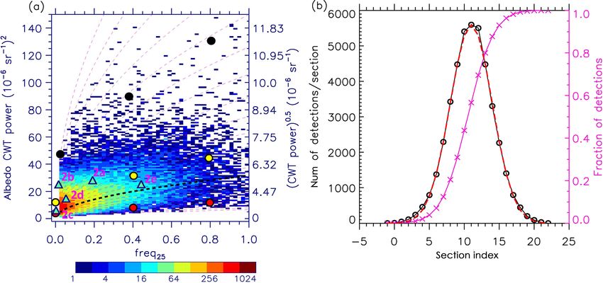
890                                                         P. Rong et al.: Universal power law of the gravity wave manifestation

Figure 4. (a) Scatterplot of the wave detections to reflect the relationship between the bright-cloud frequency (freq25 ) and the albedo CWT
power. Only detections corresponding to the brighter clouds (freq25 > 0.02) are included. The rainbow colors are the detection number
density within each bin (1freq25 = 0.02, and 1CWT = 1.0 × 10⁻¹² sr−2 ). The dashed thick black lines roughly follow the peaks of the
detection number density isopleths, serving to derive an analytic relationship between the cloud brightness and the CWT power. The turquoise
triangles correspond to the concentric waves shown in Fig. 2. The colored dots are selected roughly at the two tails and the peak of the
normal distribution and at three brightness levels of freq25 = 0, 0.4, and 0.8. These nine selections are representative of the full set of wave
detections, to further demonstrate the wave exhibition in Figs. 7–9. Using a sequence of analytic curves (magenta dashed) to resample the
wave detections, we obtain a normal distribution as is shown in (b). In (b) the black curve with the circles represents the obtained distribution
from the left panel, while the dashed red curve is the Gaussian fit. The magenta curve with crosses is the accumulated fraction of the data
points.

albedo power axis. The 2i/4 rather than a linear sequencing                lower and upper limits, suggesting an apparent dependence
is chosen to account for the fact that the data points become              of the albedo power on the background mean albedo. This
increasingly denser from being close to the albedo power                   confirms that albedo power monotonically increases with the
axis toward the freq25 axis. Figure 4b confirms that the                   background cloud brightness, except that a different analytic
resampling produces almost a precise normal distribution,                  form will be used to carry out the sectioning procedure.
and at the 11th interval it reaches the peak, which splits the                Linear sectioning lines are applied to the plane of the
wave detections in half.                                                   albedo power versus the mean background albedo to yield a
                                                                           normal distribution. The sectioning lines are emitted from the
4.4   Relationship between the albedo power and mean                       (0, 0) point, and the angular interval gradually increases from
      albedo                                                               the lower-right to upper-left corner to achieve symmetry of
                                                                           the distribution. A total of 27 intervals are used. Such a sec-
                                                                           tioning and resample procedure makes both the full set and
In this subsection we reexamine the albedo power depen-
                                                                           the dimmer subset achieve the normal distribution, shown in
dence on the background cloud brightness using the mean
                                                                           Fig. 5b, which confirms a consistent behavior between the
albedo within the elliptical region as the horizontal axis. This
                                                                           dimmer set and the full set. The peak of the normal distri-
angle of investigation provides a smoother picture because it
                                                                           bution is reached at the 12th sectioning interval. Both Fig. 5
does not use any imposed threshold (25 × 10−6 sr−1 ). Two
                                                                           and Fig. 3 (i.e., the albedo power histograms) indicate that
purposes are served by doing so. First, we tend to include the
                                                                           the dimmer subset and the full set follow a similar behavior.
wave detections with dimmer background since they take a
major fraction of the cloud population as is mentioned above.
Second, we tend to examine whether the full set of wave de-                4.5   Representative cases on the scatterplot
tections and those residing in the brighter cloud background
follow a consistent statistical relationship between the albedo            The dots of three different colors in Fig. 4a are the sample
power and the background cloud brightness.                                 selections of the wave detections for future-demonstration
   Figure 5a shows a similar scatterplot except using the                  purposes. Wave tracking yields a large number of detections,
mean albedo (within the elliptical region) as the horizon-                 and we aim at obtaining a universal law that governs the full
tal axis. The isopleths of the wave detection number density               set of wave display. The selections are made roughly at the
suggest a linear relationship between the albedo (fluctuation)             two tails and the peak of the normal distribution (Fig. 4b), la-
power and the background albedo, and we also note a strong                 beled the high-, medium-, and low-albedo-power categories.
asymmetry of the albedo power distribution between the                     Note that these categories are chosen based on the combina-

Atmos. Chem. Phys., 18, 883–899, 2018                                                          www.atmos-chem-phys.net/18/883/2018/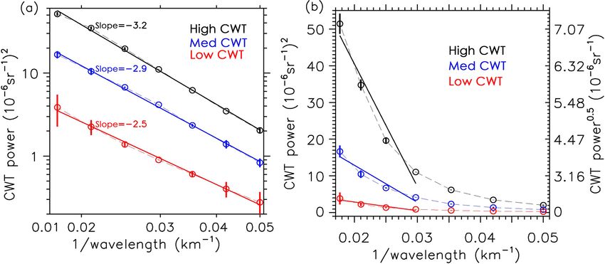
P. Rong et al.: Universal power law of the gravity wave manifestation                                                                    891

Figure 5. (a) Same as Fig. 4 except for using both dimmer and brighter sets of detections and use the mean albedo within the elliptical region
as the horizontal axis. The bin of albedo is 0.5 × 10⁻⁶ sr−1 . The turquoise triangles and colored dots are the same as in Fig. 4. (b) The
normal distributions for both the dimmer subset and the full set of wave detections. The curves without symbols are accumulated fraction of
detections with a vertical axial range of 0–1.0 (not shown), which is the same as in Fig. 4b.

tion of both albedo power and the background cloud bright-               5     Wave displays of the representative cases
ness. Three brightness levels (freq25 = 0, 0.4, and 0.8) are
used, and therefore a total of nine selections are made. The             5.1    Albedo power spectra
cases at freq25 = 0.4 and 0.8 almost precisely follow the sec-
tioning curves. While at freq25 = 0, the three selections are            The albedo power spectra of the nine selected detections are
made based on a linear relationship with the two selections              shown in Fig. 6, with the three brightness levels being col-
at freq25 = 0.4 and 0.8. This is because the dimmer subset               lapsed to each other for each albedo power category. These
(freq25 < 0.02) is not included in Fig. 4a. We should point              power spectra are calculated to extract a universal law that
out that the sectioning curves serve only as the guidance                governs the wave display. The power spectra of all orienta-
to select the cases that reasonably cover the full set of de-            tions (full 360◦ with 3◦ step) within a given elliptical region
tections, but our conclusions are not sensitive to what exact            are averaged for each individual scale in the range of ∼ 20–
cases are chosen.                                                        60 km. Although inhomogeneity exists between different ori-
   We place the same nine selected cases in Fig. 5a and find             entations, the spectra of the main wave signatures will dom-
that the three albedo power categories also roughly follow               inate the mean spectrum. Unlike the FFT power spectra that
the linear sectioning lines and are also located approximately           are prone to exhibiting spikes (not shown), the CWT power
at the lower and higher tails and at the peak of the normal              spectra have blunter features. Especially, due to the spatial
distribution.                                                            average it is even less likely that spectral peaks will stand
   At last we check on where the concentric waves shown                  out unless a given scale within the ∼ 20–60 km range is con-
in Fig. 2 are distributed on the scatterplots. From looking              sistently dominant throughout the gravity wave population,
at the turquoise-colored triangles we find that they do not              which is not the case.
seem to preferably occur at any specific combinations of                    Based on the nine representative cases, the general form
albedo power and background brightness. Rather, the five                 of power spectra can be expressed as A × (1/wavelength)α ,
cases are approximately evenly spread over the core re-                  where coefficient A = 1.42 × 10⁻⁴ , 1.45 × 10⁻⁴ , and 1.49 ×
gion, and none has occurred in either high-albedo-power or               10−4 , and the spectral exponent α = −2.5, −2.9, and −3.2
high-background-brightness ranges. Also, it is worth men-                for the low-, medium-, and high-power categories, respec-
tioning that the case of the most distinct concentric waves              tively. Note that the three categories are defined in Sect. 4.5.
shown in Fig. 2b has a combination of freq25 = 0.016 and                 For a confined range of wavelengths, i.e., ∼ 20–60 km, the
albedo power = 25.4×10⁻¹² sr−2 , suggesting that the combi-              higher wave power or larger variance level of the display will
nation of relatively low background brightness and relatively            correspond to higher clarity of wave display or to sharper fea-
high albedo power seem to correspond to the best clarity of              tures. More rapid decay toward the smaller scales will also
wave display. Although rare in occurrence and possessing                 contribute to higher display clarity because the leading scale
a known particular form of driving mechanism, concentric                 will be more dominant over the smaller scales, and therefore
waves seem to have shown a regular behavior in terms of                  the wave signature will be better organized. The actual wave
the correspondence between the albedo power and the back-                displays shown in Sects. 5.2 and 5.3 will verify these argu-
ground cloud brightness.                                                 ments.

www.atmos-chem-phys.net/18/883/2018/                                                           Atmos. Chem. Phys., 18, 883–899, 2018
892                                                           P. Rong et al.: Universal power law of the gravity wave manifestation

Figure 6. Albedo CWT power spectra for the nine detections selected in Fig. 4. The black, blue, and red colors correspond to the uppermost
row (high albedo power), middle row (medium albedo power), and the lowermost row (low albedo power) of dots in Fig. 4a, respectively.
For each albedo power category the CWT power spectra are normalized to collapse within the error bars as the 1σ standard deviation. The
exact match occurs at the medium scale (∼ 33 km wavelength or 0.03 spatial frequency) to obtain the mean slope. The thin dashed lines are
original curves, and the thicker solid lines are linear fitting lines. (a) Exponents of decay are −3.2, −2.9, and −2.5 for the three categories.
(b) Under linear axes it is shown that higher albedo power and larger exponent correspond to more rapid decay of the albedo power toward
smaller scales, reflected by the linear fitting lines for the first few dominant scales.

   The black lines in Fig. 6 are for the high-power category              levels. Measurement noise may play a role in causing this.
(see the black dots in Fig. 4a). The three brightness levels              For waves of small amplitudes and especially with very dim
possess a consistent exponent α = −3.2, and therefore via                 background, the noise will be strong enough to affect the de-
simple adjustment of A (in the analytic form) a normaliza-                termination of the wave amplitude.
tion or collapse between the three spectra is achieved. The
factors of normalization toward the brightest level are defined           5.2     Wave displays for the different albedo power
as follows:                                                                       categories

ratio0.4/0.8 = albedo powerat freq25 =0.4 /albedo powerat freq25 =0.8 ,   Before examining the wave displays, we first set the rules
                                                                   (1)    of presentation. First, a white–blue color scheme with a lin-
ratio0.0/0.8 = albedo powerat freq25 =0.0 /albedo powerat freq25 =0.8 ,   ear red–green–blue (RGB) code system is used to generate
                                                                   (2)    the color bars. Second, the mean albedo within the ellipti-
                                                                          cal region, or the background cloud brightness, is subtracted.
where albedo power refers to the total wave power over the                Third, the maximum and minimum albedo deviation is set
scales of ∼ 20–60 km. As is argued above, the normaliza-                  to be ±20.0        −6 −1
tion is carried out to examine the wave morphology beyond                            √× 10 sr for√freq25 = 0.8 and is then reduced
                                                                          by factors ratio0.4/0.8 and ratio0.0/0.8 for freq25 = 0.4 and
the wave power dependence on the background brightness.                   freq25 = 0.0, respectively. As is argued above, these factors
After applying these factors, the three brightness levels will            are expected to unify the display clarity between different
achieve a nearly fully collapsed power spectrum and exhibit               brightness levels.
the same level of display clarity (see Sect. 5.2). The black
line under the linear axes shown in Fig. 6b indicates that                5.2.1    The high-albedo-power category
the high-power category possesses both the highest overall
power level and the most rapid decay rate toward the smaller              Figure 7 presents the CIPS albedo maps and the albedo
scales.                                                                   power maps within the elliptical region for the high-albedo-
   The error bars in Fig. 6 are the uncertainty ranges over the           power category (corresponding to the black dots in Fig. 4a).
three brightness levels for the different scales, and the exact           We observe generally widespread and distinctly clear semi-
match occurs at the middle data point (i.e., ∼ 33 km of wave-             organized structures at all three brightness levels. The three
length or 0.03 of spatial frequency). It is noteworthy that both          panels show very similar levels of display clarity because
the high- and medium-albedo-power categories have very                    their albedo√power spectra are√ almost fully collapsed with
small error bars, suggesting a strong collapse of spectra at              the factors ratio0.4/0.8 and ratio0.0/0.8 being applied. The
the three brightness levels. The low-albedo-power category,               high-power category obviously possesses the overall high-
however, has notably larger error bars. This means that when              est power level, and furthermore it also has the most rapid
the albedo power reaches very low values the exponent α                   albedo power decay rate (Fig. 6b) toward the smaller scales,
maintains poorer consistency between the three brightness                 i.e., with A = 1.42 × 10⁻⁴ and α = −3.2, respectively. Both

Atmos. Chem. Phys., 18, 883–899, 2018                                                          www.atmos-chem-phys.net/18/883/2018/
P. Rong et al.: Universal power law of the gravity wave manifestation 893
Figure 7. Albedo maps and the albedo power maps corresponding to the high-power category at three different brightness levels, each with
the mean background albedo subtracted. The blue–white color scheme used linear RGB color code distribution. The albedo power maps used
the same rainbow color bar as in Fig. 2. Based on the factors used to make the albedo power spectra collapse between the different brightness
levels, which are ratio0.4/0.8 = 1.44 and ratio0.0/0.8 = 3.13, in this case (see Eqs. 1 and 2 in Sect. 5.1), the corresponding color bar maxima
√ √
are reduced by factors 1.44 = 1.2 and 3.13 = 1.77, to achieve the same level of display clarity.
conditions contribute to the fact that these displays are the brightness levels are considered to have the same level of dis-
most distinct among the three categories. In terms of mor- play clarity due to the collapse of their CWT power spectra.
phology, the wave signatures resembled straight waves or in-
terference of the straight waves, but occasionally the straight- 5.2.3 The low-albedo-power category
wave features show curvatures at certain portion of the dis-
play (in Fig. 7b and c). Overall, the wave morphology is Wave displays in the low-albedo-power category (see Fig. 9)
qualitatively consistent regardless of the brightness levels. provide firm proof that the display clarity of the wave sig-
However, looking more closely, we do perceive a minor dif- natures becomes increasingly poorer as the albedo power
ference between the low- and high-brightness display. That decreases. All panels show highly blurry features, and yet
is, at the dimmest level (freq25 = 0.0) the wave display ap- the orientations of the wave signatures remain recognizable.
pears to exhibit stronger linearity than those in the brighter Note that in this category normalizing the clarity level be-
backgrounds. From Fig. 2b we did notice that a dimmer tween different brightness levels has run into larger uncer-
background has supported highly distinct wave structures tainty because of the larger error bars (see Fig. 6a). It is
that resembled linear waves. On the contrary, the displays noticeable that the wave display for freq25 = 0 seems the
at freq25 = 0.4 and freq25 = 0.8 seem mildly turbulent-like. most blurry because under this condition both the back-
ground mean albedo and the albedo disturbances are likely
strongly affected by the measurement noise. Although dis-
5.2.2 The medium-albedo-power category
play clarity does not hold any absolute physical meaning, we
can conclude that the gravity wave signatures of ∼ 20–60 km
Figure 8 presents the maps for the medium-power category wavelength become increasingly more diffusive as the corre-
(corresponding to the yellow dots in Fig. 4a). Remember that sponding albedo power decreases. Note that Fig. 2b shows
these cases are the closest to the peak of the normal distri- that even within the same elliptical region (∼ 400 km range)
bution and therefore are the most representative of the full the wave display clarity differs drastically. This could be due
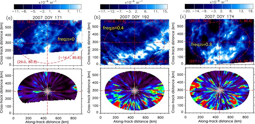
set of wave detections. The maps shown in Fig. 8 are signif- to the unknown local forcing mechanisms that have exerted
icantly blurrier than those in Fig. 7, but the wave signatures different levels of diffusion on the PMC albedo structures. So
remain well organized. In the low-brightness end (freq25 = far we have come to an understanding that semi-organized
0.0) there are interfering straight waves approximately ori- structures seem extremely widespread, with a hierarchy of
ented perpendicularly to each other. At freq25 = 0.4 the fea- different albedo power levels. This is against the belief that a
tures resemble one-directional straight wave signatures. In wave detection procedure should yield unequivocal results.
the high-brightness end (freq25 = 0.8) there are knot-like sig-
natures which are apparently deviated from the typical linear
wave signatures. Again it is worth mentioning that the three
www.atmos-chem-phys.net/18/883/2018/ Atmos. Chem. Phys., 18, 883–899, 2018894 P. Rong et al.: Universal power law of the gravity wave manifestation
Figure 8. Same as Fig. 7 except for corresponding to the medium-albedo-power category. They are systematically blurrier than those in
Fig. 7.
Figure 9. Same as Fig. 7 except for corresponding to the low-albedo-power category. They are furthermore blurrier than what is shown in
Fig. 8.
5.3 Artificially raising the medium toward high albedo ity. The previously determined A for the medium-power cat-
power egory is 1.45 × 10⁻⁴ , and in this experiment a new param-
eter Anew = 2.778 × A is used to draw closer the spectra of
The three lines with different colors in Fig. 6a have a hierar- the medium toward the high power levels. The factor 2.778
chy of albedo power levels as well as different slopes char- is chosen to maximally match the high- and medium-power
acterized by varying A and α. They, however, appear parallel spectra over the scales of ∼ 20–60 km.
to each other because the standard deviation of the exponent The result of the amplified case is shown in Fig. 10, and
α (−3.2 to −2.5) only reaches 0.3. We next systematically we used the case presented in Fig. 8a to conduct this ex-
raise the medium power level to match the high power level periment. Figure 10a shows the albedo map and the power
by increasing the coefficient A but maintain the exponent α map for the amplified case, and Fig. 10b and c are repeats
to examine how the display clarity improves. We have ar- of Figs. 8a and 7a, to make comparisons. It is shown that
gued that parameters A and α both have a control over the Fig. 10a exhibits notably improved clarity compared to its
display clarity. Carrying out this experiment is a way to test previous version, and as a result Figs. 10a and c show clar-
the role of the coefficient A in determining the display clar-
Atmos. Chem. Phys., 18, 883–899, 2018 www.atmos-chem-phys.net/18/883/2018/P. Rong et al.: Universal power law of the gravity wave manifestation 895
√
Figure 10. (a) demonstrates that amplifying the waves shown in Fig. 8a (current panel b) by a constant factor 2.778 (see text in Sect. 5.3)
enhances its display clarity significantly. The enhanced display clarity is drawn closer toward what Fig. 7a (current panel c) shows. Note that
Fig. 7a belongs to the high-albedo-power category and has the highest level of display clarity.
ity levels drawn closer, but the amplified case is still blur- to cope with a lot of challenge and uncertainty in the wave
rier. This indicates that the difference between the two ex- tracking study.
ponents (−3.2 versus −2.9) has a fundamental effect on the Figure 11a presents an example of longer and shorter
wave display clarity. Lastly, we need to point out that it is waves observed together. They are a set of bright and dim
not straightforward why exponent α varies between different cloud bands that suggest wavelengths of ∼ 150–200 km and
albedo power levels and why it remains roughly consistent shorter waves with wavelengths of ∼ 20–60 km, indicated by
along the sectioning curves used to resample the wave detec- the pairs of magenta arrows with solid heads and thin heads,
tions. The physical mechanism that governs such variability respectively. In this case the CIPS orbital strip achieves pretty
is worth a further investigation. It is probable, as we have satisfying capture of the waves because ∼ 150–200 km is
argued above, that noise contamination is one cause of the still a short wavelength relative to the cross-track span (∼
smaller slopes for lower albedo power. 900 km) of the CIPS orbital strip. The albedo map reveals
that the longer and shorter waves are nested together and the
longer waves appear to have larger amplitudes. The albedo
5.4 Explore the longer-wavelength wave display power map in the lower panel shows that the wave power is
primarily distributed in the upper-right and lower-left quad-
Longer-wavelength (> 100 km) waves are not as visually de- rants, which reflects the orientation of the wave ridges and
tectable as the shorter waves because the CIPS orbital strip troughs that is perpendicular to this.
is not able to embrace many repeats of the ridge and trough The albedo power spectra for this particular case are
of such waves. Chandran et al. (2010) used a wave detec- shown in Fig. 11b, revealing a −3.0 slope over the scale
tion algorithm to yield a peak population of waves at scales range of ∼ 20–150 km. The correspondence of freq25 = 0.34
of ∼ 250 km from the cross-track traces. Zhao et al. (2015) and albedo power = 25.0 × 10⁻¹² sr−2 makes this case the
yield a peak wavelength at ∼ 400 km from the along-track closest to the medium-albedo-power category shown above,
traces. Different traces may be the cause of the different and the −3.0 spectral slope is also close to −2.9. The spec-
peak wavelengths. Based on these studies, gravity waves of tra are not reliable in either the longwave limit (> 150 km)
all scales are likely widespread in the PMCs. The waves at or the shortwave limit (< 20 km). In the longwave limit the
< 100 km wavelengths are more visually detectable because elliptical region does not capture enough repeats of ridge and
their full displays are well captured. But these small-scale trough, and as a result the power spectra in this range often
waves possess a lower variance level than the larger-scale readily change when the CWT is applied to a much expanded
waves. Using a spectral analysis the larger scales often stand region (> 400 km) (not shown). In the shortwave limit the
out as the dominant wave events. In addition, wave event measurement noise will contaminate the PMC signals. It is
counting is not a deterministic procedure. For example, in worth mentioning that the ∼ 20–60 km scale range focused
the current study, the wave detections are forcibly confined on in this study is for the shortest waves CIPS can resolve
within the elliptical regions. Generally speaking, we have due to the ∼ 5 km spatial resolution and the signal noise lev-
www.atmos-chem-phys.net/18/883/2018/ Atmos. Chem. Phys., 18, 883–899, 2018You can also read