Unsupervised Segmentation for Terracotta Warrior with Seed-Region-Growing CNN(SRG-Net)

Unsupervised Segmentation for Terracotta
 Warrior with Seed-Region-Growing
 CNN(SRG-Net)
 YAO H U 1 , G UOHUA G ENG 1 , K ANG L I 1,* , W EI Z HOU 1,* , X INGXING
 H AO 1 AND X IN C AO 1
 1 School of Information Science and Technology, Northwest University, Xi’an 710127, Shaanxi, China
 * likang@nwu.edu.cn, mczhouwei12@gmail.com
arXiv:2107.13167v1 [cs.CV] 28 Jul 2021

 Abstract: The repairing work of terracotta warriors in Emperor Qinshihuang Mausoleum Site
 Museum is handcrafted by experts, and the increasing amounts of unearthed pieces of terracotta
 warriors make the archaeologists too challenging to conduct the restoration of terracotta warriors
 efficiently. We hope to segment the 3D point cloud data of the terracotta warriors automatically
 and store the fragment data in the database to assist the archaeologists in matching the actual
 fragments with the ones in the database, which could result in higher repairing efficiency of
 terracotta warriors. Moreover, the existing 3D neural network research is mainly focusing on
 supervised classification, clustering, unsupervised representation, and reconstruction. There
 are few pieces of researches concentrating on unsupervised point cloud part segmentation. In
 this paper, we present SRG-Net for 3D point clouds of terracotta warriors to address these
 problems. Firstly, we adopt a customized seed-region-growing algorithm to segment the point
 cloud coarsely. Then we present a supervised segmentation and unsupervised reconstruction
 networks to learn the characteristics of 3D point clouds. Finally, we combine the SRG algorithm
 with our improved CNN using a refinement method. This pipeline is called SRG-Net, which
 aims at conducting segmentation tasks on the terracotta warriors. Our proposed SRG-Net is
 evaluated on the terracotta warriors data and ShapeNet dataset by measuring the accuracy and
 the latency. The experimental results show that our SRG-Net outperforms the state-of-the-art
 methods. Our code is available at https://github.com/hyoau/SRG-Net.

 © 2021 Optical Society of America

 1. Introduction
 Nowadays, the repairing work of terracotta warriors is mainly accomplished by the handwork
 of archaeologists in Emperor Qinshihuang’s Mausoleum Site Museum. While more and more
 fragments of terracotta warriors are excavated from the site, the restoration does not have a high
 repairing efficiency. Moreover, the lack of archaeological technicians repairing the terracotta
 warriors makes it more uneasy to catch up with excavation speed. As a result, more and more
 fragments excavated from the archaeological site remain to be repaired. Terracotta Warrior is a
 3D natural structure and can be represented with a point cloud. Fortunately, with the development
 of 3D sensors (Apple Li-DAR, Kinect, and RealSense) and the improvement of hardware (GPU
 and CPU), it is possible to improve the repairing speed digitally. We can segment the 3D object
 of the terracotta warriors and store the fragments in the database. Our work aims at simplifying
 the work of researchers in the museum, making it easy to match fragments excavated from the
 site with the pre-segmented fragments in the database. To improve the efficiency of the repairing
 work, we propose an unsupervised 3D point cloud segmentation method for the terracotta warrior
 data based on convolution neural network. With the segmentation method proposed in this paper,
 the complete terracotta warriors can be segmented into fragments corresponding to various parts
 automatically, e.g., head, hand, and foot, etc. Compared with the traditional segmentation work
 by hand, the method proposed in this paper can significantly improve efficiency and accuracy.

Recently, there have been many pieces of research focusing on how to voxelize the point cloud
to make them evenly distributed in regular 3D space, and then implement 3D-CNN on them.
However, voxelization owns the high space and time complexity, and there may be quantization
errors in the process of voxelization, which would result in low accuracy. Compared with other
data formats, point cloud is a data structure suitable for 3D scene calculation of terracotta warriors.
We choose to segment the terracotta warriors in the form of point clouds (see samples in Fig. 1).

 Fig. 1. Simplified Terracotta Warrior Point Clouds

 Our terracotta warriors data is represented with { ∈ } =1
 
 , where is the feature space,
 means the features of one point, such as , , , , , (xyz coordinates and normal
value), means the number of points in one terracotta warrior 3D object. Our goal is to design a
function : → , where means the segmentation mapping labels, where { ∈ } =1 
 and
 is each point’s label after the segmentation. In our problem, { } is fixed while the mapping
function and { } are trainable. To solve the unsupervised segmentation problem, we can split
the problem into two sub-problems. Firstly, we need to design an algorithm to predict optimal
 . Secondly, we need to design a network to learn the labels { } better and make full use of
features of terracotta warrior point cloud. To get the optimal cluster labels { }, we think that a
good point cloud segmentation acts like what a human does. Intuitively, the points with similar
features or semantic meanings are easier to segment to the same cluster. In 2D images, spatially
continuous pixels tend to have similar colors or textures. In 3D point cloud, grouping spatially
continuous points with similar normal value or colors are reasonable to be given the same label
in 3D point cloud segmentation. Besides, the Euclidean distance between the points with the

same label will not be very long. In conclusion, we design two criteria to predict the { }:

 • Points with similar spatial features are desired to be given the same label.
 • The Euclidean distance between spatially continuous points should not be quite long.

 We design an SRG algorithm for learning the normal feature of point clouds as much as
possible. The experiment [1] shows that the encoder-decoder structure of FoldingNet [2] does
help neural network learn from point cloud. And DG-CNN is good at learning local features.
So we propose our SRG-Net inspired by FoldingNet [2] and DG-CNN [3] to learn part features
of terracotta warriors better. In Section 3, we describe the details of the process of assigning
labels { }. Section 4 will show that our method achieves better methods compared with other
methods. Compared with existing methods, the key contribution of our work can be summarized
as follows:

 • We design a novel SRG algorithm for point cloud segmentation to make the most of point
 cloud xyz coordinates by estimating normal features.
 • We propose our CNN inspired by DG-CNN and FoldingNet to learn the local and global
 features of 3D point clouds better.

 • We combine the SRG algorithm and CNN neural network with our refinement method and
 achieve state-of-the-art segmentation results on terracotta warrior data.
 • Our end-to-end model not only can be used in terracotta warrior point clouds but also
 can achieve quite good results on other point clouds. We also evaluate our SRG-Net on
 ShapeNet dataset.

2. Related Work
Segmentation is typical both in the 2D image and 3D point cloud processing. In image processing,
segmentation accomplishes a task that assigns labels to all the pixels in one image and clusters
them with their features. Similarly, point cloud segmentation is assigning labels to all the points
in a point cloud. The expected result is the points with the similar feature are given with the
same label.
 In terms of image segmentation, k-means is a classical segmentation method in both 2D
and 3D, which leads to partition n observations into k clusters with the nearest mean. This
method is quite popular in data mining. The graph-based method is another popular method
like Prim and Kruskal [4] which implements simple greedy decisions in segmentation. The
above methods focus on global features instead of the local differentiated features, so they usually
cannot get promising results when it comes to the complex context. Among unsupervised
deep learning methods, there are many learning features using the generative methods, such
as [5–7]. They follow the model of neuroscience, where each neuron represents a specific
semantic meaning. Meanwhile, CNN is widely used in unsupervised image segmentation. For
example, in [8], Kanezaki combines the superpixel [9] method and CNN and employs superpixel
for back propagation to tune the unsupervised segmentation results. Besides, [10] uses a spatial
continuity loss as an alternative to settle the limitation of the former work [9], whose method is
also quite valuable for 3D point cloud feature learning.
 In the field of 3D point cloud segmentation, the state-of-the-art methods for 2D images are not
quite suitable for being directly used on the point cloud. 3D point cloud segmentation methods
need to understand both the global feature and geometric details of each point. 3D point cloud
segmentation problems can be classified into semantic segmentation, instance segmentation,
and object segmentation. Semantic segmentation focuses on scene-level segmentation instance,

segmentation emphasizes object-level segmentation, and object segmentation is centered on
part-level segmentation.
 As to semantic segmentation, semantic segmentation aims at separating a point cloud into
several parts with the semantic meaning of each point. There are four main paradigms in semantic
segmentation, including projection-based methods, discretization-based methods, point-based
methods, and hybrid methods. Projection-based methods always project a 3D point cloud
to 2D images, such as multi-view [11, 12], spherical [13, 14]. Discretization-based methods
usually project a point cloud into a discrete representation, such as volumetric [15] and sparse
permutohedral lattices [16, 17]. Instead of learning a single feature on 3D scans, several methods
are trying to learn different parts from 3D scans, such as [16–18].
 The point-based network can directly learn features on a point cloud and separate them into
several parts. Point clouds are irregular, unordered, and unstructured. PointNet [19] can directly
learn features from the point cloud and retain the point cloud permutation invariance with
a symmetric function like maximum function and summation function. PointNet can learn
point-wise features with the combination of several MLP layers and a max-pooling layer. PointNet
is a pioneer that directly learns on the point cloud. A series of point-based networks has been
proposed based on PointNet. However, PointNet can only learn features on each point instead of
on the local structure. So PointNet++ is presented to get local structure from the neighborhood
with a hierarchy network [20]. PointSIFT [21] is proposed to encode orientation and reach scale
awareness. Instead of using K-means to cluster and KNN to generate neighborhoods like the
grouping method PointNet++, PointWeb [22] is proposed to get the relations between all the
points constructed in a local fully-connected web. As to convolution-based method. RS-CNN
takes a local point cloud subset as its input and maps the low-level relation to the high-level
relation to learn the feature better. PointConv [23] uses the existing algorithm, using a Monte
Carlo estimation to define the convolution. PointCNN [24] uses − transformation to
convert the point cloud into a latent and canonical order. As to point convolution methods,
Parametric Continuous Convolutional Neural Network(PCCN) [25] is proposed based on
parametric continuous convolution layers, whose kernel function is parameterized by MLPs and
spans the continuous vector space. Graph-based methods can better learn the features like shapes
and geometric structures in point clouds. Graph Attention Convolution(GAC) [26] can learn
several relevant features from local neighborhoods by dynamically assigning attention weights to
points in different neighborhoods and feature channels. Dynamic Graph CNN(DG-CNN) [3]
constructs several dynamic graphs in neighborhood, and concatenates the local and global features
to extract better features and update them each graph after each layer of the network dynamically.
FoldingNet adopts the auto-encoder structure to encode the point cloud × 3 to 1 × 512 and
decode it to × 3 with the aid of chamfer loss to construct the auto-encoder network.
 Part segmentation is more complex than semantic and instance segmentation because there are
significant geometric differences between the points with the same labels, and the number of
parts with the same semantic meanings may differ. Z. Wang et al. [27] propose VoxSegNet to
achieve promising part segmentation results on 3D voxelized data, which presents a Spatial Dense
Extraction(SDE) module to extract multi-scale features from volumetric data. Synchronized
Spectral CNN (SyncSpecCNN) [28] is proposed to achieve fine-grained part segmentation on
irregularity and non-isomorphic shape graphs with convolution. [29] is proposed to segment
unorganized noisy point clouds automatically by extracting clusters of points on the Gaussian
sphere. [30] uses three shape indexes: the smoothness indicator, shape index, and flatness index
based on a fuzzy parameterization. [31] presents a segmentation method for conventional engi-
neering objects based on local estimation of various geometric features. Branched AutoEncoder
network (BAE-NET) [32] is proposed to perform unsupervised and weakly-supervised 3D shape
co-segmentation. Each branch of the network can learn features from a specific part shape for a
particular part shape with representation based on the auto-encoder structure.

3. Proposed Method
In this paper, our input data for the terracotta warrior is in the form of 3D point clouds (see
samples in Fig. 1). Point cloud data is represented as a set of 3D points { | = 1, 2, 3... }, where
each point is a vector containing coordinates , , and other features like normal, color. Our
method contains three steps:

 1. We compute normal value with the coordinates.

 2. We use our seed-region-growing (SRG) method to pre-segment the point cloud.
 3. We use our pointwise CNN called SRG-Net self-trained to segment the point cloud with
 the refinement of pre-segmentation results.

 Given the point cloud only with 3D coordinates, there are several effective normal estimation
methods like [33] [34] [35]. In our method, we follow the simplest method in [36] because of its
low average-case complexity and quite high accuracy. We propose an unsupervised segmentation
method for the terracotta warrior point cloud by combining our seed-region-growing clustering
method with our 3D pointwise CNN called SRG-Net. This method contains two phases, SRG
segmentation and segmentation network. The problem we want to solve can be described as
follows. Firstly, the SRG algorithm is implemented on the point cloud to do pre-segmentation.
Secondly, we use SRG-Net for unsupervised segmentation with pre-segmentation labels.

3.1. Seed Region Growing
Unlike 2D images, not all point cloud data has features such as color and normal. For example,
our terracotta warriors 3D objects do not have any color feature. However, normal vectors can
be calculated and predicted by point coordinates [35]. It is worth noting that there are many
similarities and differences between color in 2D and normal features in 3D. For color features
in a 2D image, if the pixels are semantically related, the color of the pixel in the neighborhood
generally does not change a lot. For 3D point cloud normal features, compared with the color
features in 2D images, the normal values of points in the neighborhood of the point cloud often
differ. Points of neighborhood in one point cloud share similar features.
 We design a seed-region-growing method to pre-segment the point cloud based on the above
characteristics of the normal feature of the point cloud.
 First, we implement KNN to the point cloud to get the nearest neighbors of each point. Then
we initialize a random point as the start seed and add to the available points to start the algorithm.
Then we choose the first seed from the available list to judge the points in its neighborhood. If
the normal value and Euclidean distance are within the threshold we set, we think that the two
points are semantically continuous, and we can group two points into one cluster. The outline
about the SRG is given in Algorithm 1. The description of the algorithm is as follows:

 1. Input:
 (a) xyz coordinates of each point ∈ 3
 (b) normal value of each point ∈ 3
 (c) Euclidean distance of every two points ∈ 
 (d) neighborhood of each point ∈ 
 2. The randomly chosen point is added to the set , we can call it seed .

 3. For other points which are not transformed to seeds in :

(a) Each of point in seed’s neighbor , check the normal distance and Euclidean
 distance between the point in and the seed .
 (b) We set the normal distance and the Euclidean distance threshold. If both of the two
 value is less than the two thresholds, we can add it to .
 (c) The current seed is added to the checked list .

 Algorithm 1: SRG unsupervised segmentation
 Input: = { ∈ 3 } // x, y, z coordinates
 = { ∈ 3 } // normal value
 = { ∈ } // Euclidean distance
 Ω(·) // nearest neighbour function
 Output: = { ∈ 1 } // segmentation label of each point
 Initialize: :=  // set seed list to empty
 := {1, 2...| |} // select random point to available point list as seed
 for t = 1 to T do
 while ≠  do
 ← 
 ℎ ← Ω( ) for ℎ ≠  do
 ℎ ← ( ℎ )
 if ( , ℎ ) ≤ ℎ ∧ ( , ℎ ) ≤ ℎ ∧ ℎ ∉ then
 ℎ ℎ ℎ 
 else
 ℎ ℎ 
 
3.2. SRG-Net
We propose our SRG-Net, which is inspired by the dynamic graph in DG-CNN and auto-encoder
in FoldingNet. Unlike classical graph CNN, our graph is dynamic and updated in each layer of
the network. Compared with the methods that only focus on the relationship between points, we
also propose an encoder structure to better express the features of the entire point cloud, aiming
at learning the structure of the point cloud and optimize the pre-segmentation results of SRG.
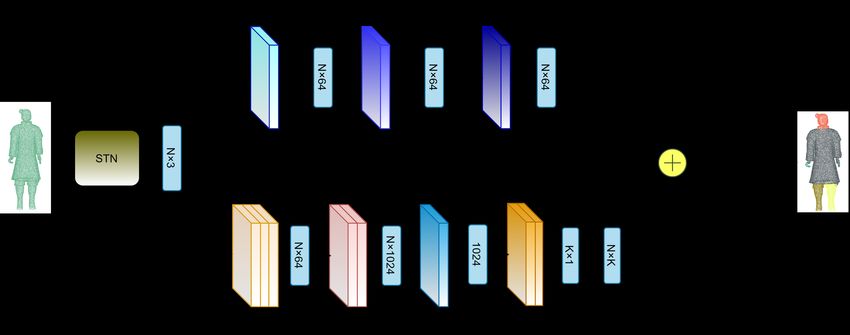
Our network structure can be shown in Fig. 2, which consists of two sub-network, the first part is
an encoder that generates features from the dynamic graph and the whole point cloud and the
second is the segmentation network.
 We denote the point cloud as . We use lower-case letters to represent vectors, such as , and
use upper-case letter to represent matrix, such as A. We call a matrix m-by-n or × if it has m
rows and n columns. In addition, the terracotta warrior point cloud data is N points with 6 features
 , , , , , (xyz coordinates and normal values), denoted as = { 1 , 2 , 3 , ..., } ⊆ 6 .

3.2.1. Encoder Architecture
The SRG-Net encoder follows a similar design of [2], the structure of SRG-Net is shown in Fig. 2.
Compared with [2], our encoder concatenate several multi-layer perceptrons(MLP) and several
dynamic graph-based max-pooling layers. The dynamic graphs are constructed by applying
KNN on point clouds.
 For the entire point cloud, we compute a spatial transformer network and get a transformer
matrix of 3-by-3 to maintain invariance under transformations. Then for the transformed point

Fig. 2. Network Structure. The brown part represents the Spatial Transformer Network,
 the blue module represents the Edge Convolution, and the lower module represents the
 Graph Convolution. The tensors of the upper and lower modules will be concatenated,
 and be input into the Segmenter to get the final segmentation result. (Segmenter will
 be explained in the following figure.)

cloud, we compute three dynamic graphs and get graph features respectively. In graph feature
extracting process, we adopt the Edge Convolution in [6] to compute the graph feature of each
layer, which uses an asymmetric edge function in Eq. (1):

 = ℎ( , − ) (1)

where it combines the coordinates of neighborhood center with the subtraction of neighborhood
point and the center point coordinates − to get local and global information of neighborhood.
Then we define our operation in Eq. (2):

 = Θ( · ( − ) + · ) (2)

where and are parameters and Θ is a ReLU function. Eq. (2) is implemented as a shared
MLP with Leaky ReLU. Then we define our max-pooling operation in Eq. (3):

 = max (3)
 ∈ ( )

where ( ) means neighborhood of point .
 The bottleneck is computed by the graph feature extraction layer. The structure is shown in
Fig. 2. First, we compute the covariance 3 × 3 matrix for every point and vectorize it to 1 × 9.
Then the × 3 matrix of point coordinates is concatenated with the × 9 covariance matrix into a
 × 12 matrix. Then we put the matrix into a 3-layer perceptron. Then we feed the output of the
perceptron to two subsequent graph layers. In each layer, max-pooling is added to the neighbor
of each node. At last, we apply a 3-layer perceptron to the former output and get the final output.
The whole process of the graph feature extraction layer is summarized in Eq. (4):

 = ( ) (4)
In Eq. (4), is the input matrix to the graph layer and is a feature mapping matrix. ( )
can be represented in Eq. 5:

 ( ( )) = Θ( max ) (5)
 ∈ ( )

Fig. 3. Edge Convolution. The figure contains a KNN graph convolution mapping the
 point cloud to N × k × f’, and then put into max-pooling to get the point cloud edge
 feature.

where Θ is a ReLU function and ( ) is the neighborhood of point . The max-pooling operation
in Eq. (5) can get local feature based on the graph structure. So the graph feature extraction layer
can not only get local neighborhood features, but also global features.

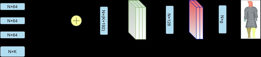
3.2.2. Segmenter Architecture

 Fig. 4. Segmenter Structure. First, the segmenter concatenates the features calculated
 by edge convolution and graph convolution. Then put into three-layer-perceptron, and
 finally put into two-layer-perceptron to get the final segmentation result.

 Segmenter gets dynamic graph features and bottleneck as input and assign labels to each point
to segment the whole point cloud. The structure of segmenter is shown in Fig. 2. First, bottleneck
is replicated times in Eq. (6):
 0 = ∪ ∪ ... ∪ (6)
 | {z }
 
where is the number of points in point cloud and is the bottleneck. The output of replication
is concatenated with dynamic features in Eq. (7):

 = 0 ∪ 1 ∪ 2 ∪ 3 (7)

where 1 , 2 , 3 represent dynamic graph features. At last, we feed the output of concatenation
to a multi-layer-perceptron to segment the point cloud in Eq. (8).

 = Θ(Ψ · + Ω) (8)

where Ψ and Ω represent parameters in the linear function, and Θ represents a ReLU function.

3.3. Refinement
Inspired by [37], we designed point refinement to achieve better segmentation results. The basic
concept of point clustering is to group similar points into clusters. In point cloud segmentation,
it is intuitive for the clusters of points to be spatially continuous. We add the constraint to favor

cluster labels that are the same as those of neighboring points. We first extract superpoints
{ } 
 =1 from the input point cloud = { } =1 , where is a set of the indices of points that
 
belongs to the k-th superpoint. Then we assign points in each superpoint to have the same cluster
label. More specifically, letting | | ∈ be the number of points in that belong to the th
cluster, we select the most frequent cluster label , where | | ∈ ≥ | | ∈ for all
 1, ..., . The cluster labels are replaced by for ∈ .
 In this paper, there is no need to set a large number in seed-region-growing process because
our neural network can learn both the local and global features. We choose seed-region-growing
method with = 25 for the super point extraction. The refinement process can achieve better
results compared with straight learning in Fig. 1. In addition, instead of using ground truth to
calculate loss, we use the coarse segmentation result of seed-region-growing method to calculate
the loss.

4. Experiments
We conduct experiments on terracotta warrior dataset and ShapeNet dataset. We implement the
pipeline using PyTorch and Python3.7. All the results are based on experiments under RTX
2080 Ti and i9-9900K. The performances of each method in the experiment are evaluated by the
accuracy (mIoU) and the latency.

4.1. Experiments on Terracotta Warrior
We use Artec Eva [38] to collect 500 intact terracotta warrior models, and we take 400 of the 500
models as the training set and 100 as the validation set. Each model consists of about 2 million
points which include xyz coordinates, vertical normals, triangle meshes and RGB data. Before
the experiments start, we eliminate the triangle meshes and RGB data of the original models, and
remain xyz coordinates and vertical normals. Moreover, we uniformly sample the above point
clouds to 10,000 points thus as the experimental inputting. In reality, the terracotta warriors are
generally unearthed in the form of limb fragments.
 To better assist the restoration of terracotta warriors, we split the point cloud into six pieces both
in SRG and K-Means. We also set the number of iterations as 2000 in each method(PointNet [19],
PointNet2 [20], DG-CNN [3], PointHop++ [39], ECC [40]) for every point cloud. Unlike the
supervised problem, our unsupervised method solves two sub-problems: prediction of cluster
labels with fixed network parameters and training of network with predicted labels. The former
sub-problem is solved with Section 3.3. The latter sub-problem is solved with back-propagation.
 We select SGD as optimizer, choose = 0.005, and set the momentum factor to 0.1. To
make fair comparison in the experiments, we combine PointNet [19], PointNet2 [20], DG-
CNN [3], PointHop++ [39] with the seed region growing method to have a similar structure of
SRG-Net. In addition, the seed region growing is also compared with K-means. Comparison
of different methods is shown in Table 2, and the visualization results of different methods
are presented in Table 1. As is shown in Table 1, compared with k-means methods(K-means-
DGCNN, K-means-Pointnet2, K-means-Pointnet), our seed-region-growing method can get
roughly correct segmentation results. In contrast, k-means methods get the wrong segmentation
results. Compared with SRG-DGCNN, SRG-PointNet2, SRG-PointNet, our SRG-Net can get
more accurate segmentation results.
 As shown in Table 2, SRG-Net outperforms SRG-DGCNN by increasing more than 5.5% of
accuracy with consuming about 50% of SRG-DGCNN latency. Our method also outperforms
SRG-PointHop++ and SRG-ECC by a large margin(6.1%, 8.2%) with about 72.2% and 70.3%
latency. Compared with K-means methods, SRG-Net improves SRG-ECC and SRG-DGCNN by
more than 10% in mIoU, and it also outperforms Kmeans-PointNet2 and K-means&PointNet by
a large margin.
 Ranking the results of different methods in Table 2, we can draw the following conclusions:

Method 005413 005420 005422 005423 005427 005455

 SRG-
DGCNN

 SRG-
Pointnet2

 SRG-
Pointnet

K-means-
DGCNN

K-means-
Pointnet2

Kmeans-
Pointnet

SRG-Net

 Table 1. Visualization Results of Different Methods on Terracotta Warrior

Method Accuracy(%) Latency(ms)

 SRG-DGCNN 78.32 37.26
 SRG-PointHop++ 77.94 30.62
 SRG-ECC 76.32 31.45
 SRG-Pointnet 72.03 13.35
 SRG-Pointnet2 70.55 24.10

 K-means-DGCNN 70.64 36.30
 K-means-Pointnet2 52.33 25.38
 K-means-Pointnet 53.94 13.47

 SRG-Net 82.63 22.11

 Table 2. Comparison of Different Methods

 1. Compared with SRG-DGCNN, SRG-PointNet, SRG-PointNet2, our network can enhance
 the accuracy of learning with less latency.
 2. Compared with Kmeans-DGCNN, Kmeans-PointNet, Kmeans-PointNet2, our customized
 SRG method can achieve better results compared with k-means.
 3. In general, SRG-Net has obvious advantages in accuracy and latency.

4.2. Experiments on ShapeNet
In this section, we perform experiments on ShapeNet to evaluate the robustness of our SRG-Net
method. ShapeNet contains 16,881 objects from 16 categories. We set the number of the parts
according to different categories separately. All models were down-sampled to 2,048 points. The
evaluation metric is mean intersection-over-union (mIoU).
 Our quantitative experiment results are shown in Table 3. As in Table 3, SRG-Net outperforms
all previous models. SRG-Net improves the overall accuracy of SRG-DGCNN by 8.2% and
even larger overhead compared with SRG-PointNet2 and SRG-PointNet. Especially, our method
outperforms SRG-DGCNN on all kinds of categories, increasing 5% accuracy on knife. Overall,
our method achieves better accuracy on ShapeNet compared with other methods.
 Some visualization results are shown in Fig. 5. As is shown in Fig. 5, SRG-Net achieves
good results on bag, knife, motorbike, and achieves quite good results on airplane, earphone and
laptop.

 Method Airplane Bag Earphone Knife Laptop Bike Mug OA

 SRG-DGCNN 67.7393 61.2568 56.0633 77.0035 75.8854 70.7194 59.3024 72.6273
 SRG-Pointnet2 61.1865 54.4515 51.6673 71.9515 69.9074 64.3308 53.8897 66.4712
 SRG-Pointnet 57.1590 51.0517 47.2101 67.9229 66.4234 61.2438 49.1265 61.4242
 SRG-Net 73.0493 67.0935 62.4256 83.2430 82.6076 76.7677 65.8810 78.1954

 Table 3. Accuracy(%) of Different Methods on ShapeNet

Fig. 5. SRG-Net Segmentation Results of ShapeNet

4.3. Ablation Study
In order to show the influence of different modules and epochs in our method, we conduct
ablation studies on our terracotta warrior dataset, which are described in Section 3.2, which are
evaluated by overall accuracy and mIoU.
 The influences of different modules. As shown in Table 4, The results of version without the
graph convolution (A, row 1) show that the network not working well in learning the topological
features of the local neighborhood of the point cloud. The results of version without edge
convolution (B, row 2) demonstrate that our method without edge convolution will cause the
network unable to understand the relationship between points well. The results of version without
refinement operation (C, row 3) reveal that the pipeline cannot set tags reasonably based on point
cloud content because the number of unique cluster labels should be adaptive to context. The
results show that the refinement operation increase 15.6% on the accuracy of SRG-Net.
 The influences of different epochs. To visualize the influence of different epochs, we set the
number of epochs to 2500 and set the segmentation number to 6. The segmentation results of
different iterations in one terracotta warrior model are shown in Fig. 6.

 Method mIoU(%) OA(%)

 A 77.71 80.17
 B 74.18 76.51
 C 71.46 73.48

 Table 4. Ablation Study

(a) iter 250 (b) iter 500 (c) iter 750 (d) iter 1000 (e) iter 1250 (f) iter 1500 (g) iter 1750 (h) iter 2000

 Fig. 6. Results of Different Iterations in SRG-Net

5. Conclusion
This paper provides an end-to-end model called SRG-Net for unsupervised segmentation on the
terracotta warrior point cloud. Our method aims at assisting the archaeologists in speeding up the
repairing process of terracotta warriors. Firstly, we design a novel seed-region-growing method
to pre-segment point clouds with coordinates and normal value of the 3D terracotta warrior point
clouds. Based on the pre-segmentation process, we proposed a CNN inspired by the dynamic
graph in DG-CNN and auto-encoder in FoldingNet to learn the local and global characteristics
of the 3D point cloud better. At last, we propose a refinement process and append it after the
CNN process. Finally, we evaluate our method on the terracotta warrior data, and we outperform
the state-of-the-art methods with higher accuracy and less latency. Besides, we also conduct
experiments on the ShapeNet, which demonstrates our approach is also useful for the human
body and standard object part segmentation. Our work still has some limitations. The number of
points from the hand of the terracotta warrior is relatively small, so it is difficult for SRG-Net to
learn the characteristics of hands. We will try to work on this problem in the future. We hope our
work can be helpful to the research of terracotta warriors in archaeology and point cloud work of
other researchers.

6. Acknowledgments
This work is equally and mainly supported by the National Key Research and Development
Program of China (No. 2019YFC1521102, No. 2019YFC1521103) and the Key Research and
Development Program of Shaanxi Province (No. 2020KW-068). Besides, this work is also partly
supported by the Key Research and Development Program of Shaanxi Province (No.2019GY-215,
No.2019ZDLSF07-02, No.2019ZDLGY10-01), the Major research and development project
of Qinghai(No. 2020-SF-143), the National Natural Science Foundation of China under Grant
(No.61701403,No.61731015) and the Young Talent Support Program of the Shaanxi Association
for Science and Technology under Grant (No.20190107).

Disclosures
The authors declare no conflicts of interest.

References
1. A. Tao, “Unsupervised point cloud reconstruction for classific feature learning,”
 https://github.com/AnTao97/UnsupervisedPointCloudReconstruction (2020).
2. Y. Yang, C. Feng, Y. Shen, and D. Tian, “Foldingnet: Point cloud auto-encoder via deep grid deformation,” in
 Proceedings of the IEEE Conference on Computer Vision and Pattern Recognition, (2018), pp. 206–215.
3. Y. Wang, Y. Sun, Z. Liu, S. E. Sarma, M. M. Bronstein, and J. M. Solomon, “Dynamic graph cnn for learning on
 point clouds,” Acm Transactions On Graph. (tog) 38, 1–12 (2019).
4. J. B. Kruskal, “On the shortest spanning subtree of a graph and the traveling salesman problem,” Proc. Am. Math.
 society 7, 48–50 (1956).
5. H. Lee, P. Pham, Y. Largman, and A. Ng, “Unsupervised feature learning for audio classification using convolutional
 deep belief networks,” Adv. neural information processing systems 22, 1096–1104 (2009).

6. Q. V. Le, “Building high-level features using large scale unsupervised learning,” in 2013 IEEE international
 conference on acoustics, speech and signal processing, (IEEE, 2013), pp. 8595–8598.
7. H. Lee, R. Grosse, R. Ranganath, and A. Y. Ng, “Convolutional deep belief networks for scalable unsupervised
 learning of hierarchical representations,” in Proceedings of the 26th annual international conference on machine
 learning, (2009), pp. 609–616.
8. A. Kanezaki, “Unsupervised image segmentation by backpropagation,” in 2018 IEEE international conference on
 acoustics, speech and signal processing (ICASSP), (IEEE, 2018), pp. 1543–1547.
9. R. Achanta, A. Shaji, K. Smith, A. Lucchi, P. Fua, and S. Süsstrunk, “Slic superpixels compared to state-of-the-art
 superpixel methods,” IEEE transactions on pattern analysis machine intelligence 34, 2274–2282 (2012).
10. W. Kim, A. Kanezaki, and M. Tanaka, “Unsupervised learning of image segmentation based on differentiable feature
 clustering,” IEEE Transactions on Image Process. 29, 8055–8068 (2020).
11. F. J. Lawin, M. Danelljan, P. Tosteberg, G. Bhat, F. S. Khan, and M. Felsberg, “Deep projective 3d semantic
 segmentation,” in International Conference on Computer Analysis of Images and Patterns, (Springer, 2017), pp.
 95–107.
12. A. Boulch, B. Le Saux, and N. Audebert, “Unstructured point cloud semantic labeling using deep segmentation
 networks.” 3DOR 2, 7 (2017).
13. B. Wu, A. Wan, X. Yue, and K. Keutzer, “Squeezeseg: Convolutional neural nets with recurrent crf for real-time
 road-object segmentation from 3d lidar point cloud,” in 2018 IEEE International Conference on Robotics and
 Automation (ICRA), (IEEE, 2018), pp. 1887–1893.
14. A. Milioto, I. Vizzo, J. Behley, and C. Stachniss, “Rangenet++: Fast and accurate lidar semantic segmentation,” in
 2019 IEEE/RSJ International Conference on Intelligent Robots and Systems (IROS), (IEEE, 2019), pp. 4213–4220.
15. B. Graham, M. Engelcke, and L. Van Der Maaten, “3d semantic segmentation with submanifold sparse convolutional
 networks,” in Proceedings of the IEEE conference on computer vision and pattern recognition, (2018), pp. 9224–9232.
16. A. Dai and M. Nießner, “3dmv: Joint 3d-multi-view prediction for 3d semantic scene segmentation,” in Proceedings
 of the European Conference on Computer Vision (ECCV), (2018), pp. 452–468.
17. M. Jaritz, J. Gu, and H. Su, “Multi-view pointnet for 3d scene understanding,” in Proceedings of the IEEE International
 Conference on Computer Vision Workshops, (2019), pp. 0–0.
18. S. Wang, S. Suo, W.-C. Ma, A. Pokrovsky, and R. Urtasun, “Deep parametric continuous convolutional neural
 networks,” in Proceedings of the IEEE Conference on Computer Vision and Pattern Recognition, (2018), pp.
 2589–2597.
19. C. R. Qi, H. Su, K. Mo, and L. J. Guibas, “Pointnet: Deep learning on point sets for 3d classification and segmentation,”
 in Proceedings of the IEEE conference on computer vision and pattern recognition, (2017), pp. 652–660.
20. C. R. Qi, L. Yi, H. Su, and L. J. Guibas, “Pointnet++: Deep hierarchical feature learning on point sets in a metric
 space,” in Advances in neural information processing systems, (2017), pp. 5099–5108.
21. M. Jiang, Y. Wu, T. Zhao, Z. Zhao, and C. Lu, “Pointsift: A sift-like network module for 3d point cloud semantic
 segmentation,” arXiv preprint arXiv:1807.00652 (2018).
22. H. Zhao, L. Jiang, C.-W. Fu, and J. Jia, “Pointweb: Enhancing local neighborhood features for point cloud processing,”
 in Proceedings of the IEEE Conference on Computer Vision and Pattern Recognition, (2019), pp. 5565–5573.
23. W. Wu, Z. Qi, and L. Fuxin, “Pointconv: Deep convolutional networks on 3d point clouds,” in Proceedings of the
 IEEE Conference on Computer Vision and Pattern Recognition, (2019), pp. 9621–9630.
24. Y. Li, R. Bu, M. Sun, W. Wu, X. Di, and B. Chen, “Pointcnn: Convolution on X-transformed points,” (2018).
25. S. Wang, S. Suo, W.-C. Ma, A. Pokrovsky, and R. Urtasun, “Deep parametric continuous convolutional neural
 networks,” in Proceedings of the IEEE Conference on Computer Vision and Pattern Recognition, (2018), pp.
 2589–2597.
26. P. Veličković, G. Cucurull, A. Casanova, A. Romero, P. Lio, and Y. Bengio, “Graph attention networks,” arXiv
 preprint arXiv:1710.10903 (2017).
27. Z. Wang and F. Lu, “Voxsegnet: Volumetric cnns for semantic part segmentation of 3d shapes,” IEEE transactions on
 visualization computer graphics (2019).
28. L. Yi, H. Su, X. Guo, and L. J. Guibas, “Syncspeccnn: Synchronized spectral cnn for 3d shape segmentation,” in
 Proceedings of the IEEE Conference on Computer Vision and Pattern Recognition, (2017), pp. 2282–2290.
29. Y. Liu and Y. Xiong, “Automatic segmentation of unorganized noisy point clouds based on the gaussian map,”
 Comput. Des. 40, 576–594 (2008).
30. L. Di Angelo and P. Di Stefano, “Geometric segmentation of 3d scanned surfaces,” Comput. Des. 62, 44–56 (2015).
31. P. Benkő and T. Várady, “Segmentation methods for smooth point regions of conventional engineering objects,”
 Comput. Des. 36, 511–523 (2004).
32. Z. Chen, K. Yin, M. Fisher, S. Chaudhuri, and H. Zhang, “Bae-net: Branched autoencoder for shape co-segmentation,”
 in Proceedings of the IEEE International Conference on Computer Vision, (2019), pp. 8490–8499.
33. D. OuYang and H.-Y. Feng, “On the normal vector estimation for point cloud data from smooth surfaces,” Comput.
 Des. 37, 1071–1079 (2005).
34. J. Zhou, H. Huang, B. Liu, and X. Liu, “Normal estimation for 3d point clouds via local plane constraint and
 multi-scale selection,” Comput. Des. 129, 102916 (2020).
35. Y. Wang, H.-Y. Feng, F.-É. Delorme, and S. Engin, “An adaptive normal estimation method for scanned point clouds
 with sharp features,” Comput. Des. 45, 1333–1348 (2013).

36. R. B. Rusu and S. Cousins, “3d is here: Point cloud library (pcl),” in 2011 IEEE international conference on robotics
 and automation, (IEEE, 2011), pp. 1–4.
37. A. Kanezaki, “Unsupervised image segmentation by backpropagation,” in 2018 IEEE international conference on
 acoustics, speech and signal processing (ICASSP), (IEEE, 2018), pp. 1543–1547.
38. A. Europe, “3d object scanner artec eva | best structured-light 3d scanning device,” .
39. M. Zhang, Y. Wang, P. Kadam, S. Liu, and C.-C. J. Kuo, “Pointhop++: A lightweight learning model on point sets
 for 3d classification,” arXiv preprint arXiv:2002.03281 (2020).
40. M. Simonovsky and N. Komodakis, “Dynamic edge-conditioned filters in convolutional neural networks on graphs,”
 in CVPR, (2017).