Unveiling the Nottingham Inversion Instability during the thermo field emission from refractory metal micro protrusions - Nature
←
→
Page content transcription
If your browser does not render page correctly, please read the page content below
www.nature.com/scientificreports
OPEN Unveiling the Nottingham
Inversion Instability
during the thermo‑field
emission from refractory metal
micro‑protrusions
Darius Mofakhami1,2,3*, Benjamin Seznec3, Tiberiu Minea3, Romaric Landfried1,2,
Philippe Testé1,2 & Philippe Dessante1,2
The electron emission by micro-protrusions has been studied for over a century, but the complete
explanation of the unstable behaviors and their origin remains an open issue. These systems often
evolve towards vacuum breakdown, which makes experimental studies of instabilities very difficult.
Modeling studies are therefore necessary. In our model, refractory metals have shown the most
striking results for discontinuities or jumps recorded on the electron emitted current under high
applied voltages. Herein, we provide evidence on the mechanisms responsible for the initiation of a
thermal instability during the field emission from refractory metal micro-protrusions. A jump in the
emission current at steady state is found beyond a threshold electric field, and it is correlated to a
similar jump in temperature. These jumps are related to a transient runaway of the resistive heating
that occurs after the Nottingham flux inversion. That causes the hottest region to move beneath the
apex, and generates an emerging heat reflux towards the emitting surface. Two additional conditions
are required to initiate the runaway. The emitter geometry must ensure a large emission area and
the thermal conductivity must be high enough at high temperatures so that the heat reflux can
significantly compete with the heat diffusion towards the thermostat. The whole phenomenon, that
we propose to call the Nottingham Inversion Instability, can explain unexpected thermal failures and
breakdowns observed with field emitters.
Modern and future ultra-high-voltage vacuum equipment requires ever better electrical insulation. This is espe-
cially true for particle a ccelerators1,2 and neutral beam injectors for t okamaks3, as well as other high-voltage
direct current devices. Unfortunately, under exceptionally high applied electric fields (107–109 V/m), several
well-identified physical phenomena can cause a series of interdependent events often evolving towards a vacuum
breakdown. Most of these breakdown events are related to the presence on the cathode of micro/nano-protru-
sions, whose shape and density depend on the surface r oughness4. Besides, such protrusions may also emerge
and evolve via electromigration5 and field-induced surface atom d iffusion6. Locally enhancing at their apex the
high applied electric field, these protrusions act as field electron emitters. Above a certain field magnitude, the
current density inside these emitters becomes high enough to generate self-heating via a combination of both
resistive heating in the emitter volume (Joule heating) and the Nottingham effect at the emission s urface7,8.
Let us recall the Nottingham effect comes from the energy balance between the mean energy of the emitted
electrons ǫout
and that of the replacing electrons ǫin
, the so-called Nottingham energy WN = �ǫin � − �ǫout �.
It yields a heat flux at the metal/vacuum interface whose magnitude depends on the emitter current density J,
according to the formula �N = −WN × J/e where e is the elementary charge. Therefore, the sign of this heat
flux can reverse. At a given field magnitude, the heat flux is positive (heating) below a certain temperature and
reverses above, becoming negative (cooling). The inversion temperature is called the Nottingham temperature and
1
Laboratoire de Génie Electrique et Electronique de Paris, Université Paris-Saclay, CentraleSupélec, CNRS,
91192 Gif‑sur‑Yvette, France. 2Laboratoire de Génie Electrique et Electronique de Paris, Sorbonne Université,
CNRS, 75252 Paris, France. 3Laboratoire de Physique des Gaz et des Plasmas, Universite Paris-Saclay, CNRS,
91405 Orsay, France. *email: darius.mofakhami@centralesupelec.fr
Scientific Reports | (2021) 11:15182 | https://doi.org/10.1038/s41598-021-94443-7 1
Vol.:(0123456789)www.nature.com/scientificreports/
is analytically found proportional to the local electric field magnitude and inversely proportional to the square
root of the emitter work function7: TN ∝ F/ϕ 1/2.
Because higher temperatures facilitate the emission of electrons, it is well established that the self-heating
of an emitting protrusion may lead to a vacuum breakdown, following different possible scenarios. If the tem-
perature at the emitter apex reaches the melting point, vapor will be released. Its ionization by the energetic
emitted electrons in front of the protrusion can then ignite an arc, possibly yielding a breakdown9,10. Another,
less frequent, possibility could be the explosion of the protrusion, namely with RF fi elds11,12, due to a much faster
increase of the temperature and/or the maximum temperature reached below the apex, in the emitter volume13.
On the other hand, a high thermo-field current from the cathode can also locally heat the anode and cause the
detachment of adsorbed microparticles, which then collide the cathode (the micro-protrusions), following the
Cranberg scenario14–16.
Similar thermal instabilities during field emission are also an issue for modern electron sources’ design. Since
the last decades, efficient vacuum electron sources based on optimally spaced arrays of sharp field emitters pur-
posely grown at a cathode surface offer higher integrability, commutability and durability than their thermionic
counterparts17–19. However, the emitter self-heating during thermo-field emission limits the operation voltage,
capping the emitted current performances20–23. Hence, the question of thermal stability in the self-heating process
of field-emitting protrusion is an issue for both the domain of field electron sources and high-voltage vacuum
insulation.
Unfortunately, it is technologically very difficult—even impossible—to perform reproducible experiments
close to the breakdown while locally track the heat-related quantities at the individual emitter scale. Besides,
the damages caused onto the system in case of a breakdown generally have critical consequences. Therefore,
analytical works have been conducted in parallel with the experiments to get general insights into the self-heating
process24–27. Nevertheless, considering the problem complexity—related to the solving on a real geometry of
the coupled equations of heat and current—many simplifying assumptions are necessary. Most of the published
solutions reduce the system to only one dimension (1D), often stationary, and not or only partially taking into
account the Nottingham effect—Notice that the Nottingham effect varies with the surface temperature, making
the equation system self-consistent, since the boundary condition (the Nottingham heat flux) is function of the
solution (the surface temperature). Therefore, we should rather focus our overview on multi-physics model of
the self-heating process.
Relying on the ever-increasing computing power, several numerical models have followed one another since
the ’80s. They brought insights into the heating evolution in time28–30 along with more accurate considerations
of the underlying quantum d ynamics31–33. Concerning the contribution of the Nottingham effect to the emitter
self-heating, modeling works have shown that it was predominant over the resistive heating at low current density,
while the situation reverses at higher density34,35. Once the apex temperature exceeds the Nottingham inversion
temperature, the cooling Nottingham effect even causes the maximum temperature to sink beneath the surface,
as highlighted by Fursey13 and Rossetti et al.36. However, these studies overall lacked a detailed description in
time of the various heating terms and an exhaustive exploration of the applied voltage (or electric field).
To go further, our work investigates the self-heating evolution during the electron emission from single pro-
trusions. For each protrusion, the whole thermo-field regime is explored, up until the melting point is reached.
The focus goes on an unstable thermal behavior of refractory metal protrusions related to the Nottingham heat
flux inversion. Once a threshold electric field is exceeded, a runaway of the self-heating process occurs, drastically
facilitating the emitter thermal failure or even directly causing it. The whole phenomenon, not documented so
far, is proposed to be called the Nottingham Inversion Instability. It is shown to be caused by threshold feedback
mechanisms that depends on the emitter geometry and specific material properties. Thus, besides its contribu-
tion to the domain of electron sources and vacuum breakdowns, this work sheds some light on the possible
nonlinear evolution of self-consistently coupled equations, which present a fundamental interest in the field of
complex system dynamics.
Emission model
Our model uses a finite element approach to reproduce any 3D geometry and a time-dependent solver based on
the Backward Differentiation Formula method. In this paper, the analysis is focused on the thermal evolution of
single axially symmetric protrusions, located on a plane cathode and facing a plane anode
(Fig. 1). The applied
voltage is denoted Vapp and a time ramp is set so that Vapp (t) = Vapp 1 − exp(−t/τ ) with the time constant
τ = 1 ns to correctly simulate the initiation of field emission. The corresponding applied electric field is deduced
from the distance Dgap = 200 µm between the cathode and the anode: E = Vapp /Dgap. The local electric field F
at the emitter surface is obtained by solving the Laplace equation in the vacuum gap (space-charge is not taken
into account) :
Vvac = 0 , � vac
F� = −∇V (1)
where Vvac is the voltage inside the vacuum chamber. The field enhancement factor at the emitter apex is denoted
β , so that the local field there writes Fa = βE.
Together with the material work function ϕ and the temperature T (initially at room temperature), the field
magnitude is used to numerically compute the emitted current density J(F, T, ϕ) by integrating over all normal
energy the product between the supply function and the transmission probability. The supply function is obtained
within the framework of the Sommerfeld theory while the transmission probability is computed following the
Kemble formalism37, assuming a 1D potential barrier corrected by the image charge: the so-called Schottky–Nor-
dheim Barrier. Detailed formulas can be found in our previous w ork38, appendix A therein. Note that the 1D
approximation does not hold for curvature radii below 20 nm30. However, our study limits to curvature radii
Scientific Reports | (2021) 11:15182 | https://doi.org/10.1038/s41598-021-94443-7 2
Vol:.(1234567890)www.nature.com/scientificreports/
Figure 1. Scheme of the simulation domain in a 2D sectional view along the radial coordinate r (not at scale).
The domain is bound between [Lcat , Lz ] along the symmetry z-axis, and between [0, Lr ] along the r-axis. The
boundary conditions are shown in blue for the Laplace equation (solved in the vacuum gap) and respectively in
red and purple for the heat and current equations (solved in the cathode). The green dashed line highlight the
cathode-vacuum interface. The field emission related quantites at the interface are highlighted in green.
down to 39 nm (taking the Gaussian curvature H/f 2 for the hemiellipsoid with H = 10 µm and f = 16). The
Nottingham heat flux �N (F, T) = −WN × J/e is then deduced from the emission current density J and the Not-
tingham energy WN , assuming a mean energy equal to the Fermi level for the replacement electrons.
Both the Nottingham heat flux and the emission current density are used as von Neumann boundary condi-
tions at the cathode upper surface (i.e. the vacuum–cathode interface, see the green dashed line in Fig. 1) to solve
the time evolution of the coupled equations of heat:
2
ρ(T)c(T)
∂T � · φ� = j ,
−∇ �
φ� = −κ(T)∇T (2)
∂t σ (T)
and current:
� · �j = 0 , ∂ �
∇ �j = σ (T) + ε0 ∇Vcat (3)
∂t
where ρ , c, κ and σ respectively denote the volumetric mass density, the specific heat capacity, the thermal con-
ductivity and the electrical conductivity of the cathode material, all being temperature-dependent (see “Material
properties”). Note that the thermal losses due to surface radiation are negligible in all analyzed cases. At the
cathode lower surface, Dirichlet boundary conditions are set assuming constant temperature and potential. Far
away on the simulation box lateral boundary, symmetry conditions are enforced. At each time step, the field
and temperature at the emitter surface are updated and the self-heating process is simulated until a steady state
is reached or no convergence is found. All boundary conditions are shown in Fig. 1.
Results
Discontinuous transition between two steady states. Although our model is able to deal with 3D
arrangements of emitters38, for the sake of clarity and reduced computation time, the results presented hereafter
were obtained with a single axisymmetric protrusion. Note that the highlighted phenomena would occur in a
similar way with more complex 3D geometries, as long as the conditions detailed later on in the discussion are
fulfilled. Let us therefore start with the case of a tungsten hemiellipsoid emitter, with the work function taken to
φ = 4.5 eV, height H = 10 µm and base radius R = 1 µm, which gives an aspect ratio f = H/R = 10 and an
apex field enhancement factor β = 49.3 (Fig. 2a).
First, Fig. 2b shows the increase of both the temperature at the emitter apex Ta and the maximum temperature
inside the emitter Tmax , at steady state, versus the applied electric field E . Being interested in the self-heating
process, we explore fields covering all the possible range for the maximum temperature, from room temperature
(∼ 300 K) up to the melting point of tungsten Tm = 3695 K. The corresponding current densities are shown
in Fig. 2c with Jmax being the maximum emission current density released from the emitter surface, essentially
located at the apex. Surprisingly, the curves exhibit a sudden jump in both temperatures and in current density,
denoted Ta , Tmax and Jmax respectively. These jumps occur at a certain value of the applied electric field,
Scientific Reports | (2021) 11:15182 | https://doi.org/10.1038/s41598-021-94443-7 3
Vol.:(0123456789)www.nature.com/scientificreports/
Figure 2. Highlight of a temperature jump versus the applied electric field in the steady state thermo-field
emission of a tungsten hemiellipsoid. (a) Sketch of the emitter. β is the apex field enhancement factor, so that the
locally enhanced electric field at the apex is F = βE , where E is the applied electric field. The dimensions are not
at scale. (b) Variation of the emitter maximum temperature Tmax and its apex temperature Ta versus the applied
electric field. (c) Variation of the maximum emitted current density Jmax versus the applied electric field. Each
data point is the result at steady state of a transient simulation where the field is raised from zero to the indicated
x-axis value over a few nanoseconds. (b’,c’) are zooms of (b,c) framed areas, respectively.
named hereafter the threshold applied electric field Eth . In addition, below Eth , the maximum temperature equals
the apex one, meaning the apex is the hottest point of the emitter. However, above Eth the maximum temperature
significantly exceeds the apex temperature, which may sound counterintuitive at first glance since the Joule heat-
ing is still maximal at the apex. From the numerical point of view, all these solutions did converge well, but it was
not possible to reach a steady state with a maximum temperature in the jump region. That is why we assimilate
this jump to an instability caused by the coupled evolution of several terms in the equation system. Refining the
field sampling around the threshold down to a step δ =5 kV/m gives a value of Eth = 201.785 MV/m. The related
jumps in temperature are then Tmax = 843 K and Ta = 311 K, meaning the maximum temperature separates
from the apex by about 500 K. After this jump, it is important to note that the maximum temperature still has
not exceeded the melting temperature. Therefore, all the simulations are physically valid up until they exceed
the horizontal red line at TM = 3695 K. This occurs for a pre-breakdown electric field, Epb = 202.25 MV/m.
Beyond Epb, additional physics come into play that will eventually lead to a breakdown (gray crosses beyond
Epb, Fig. 2b-inset).
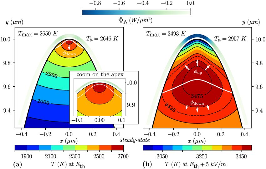
Second, Fig. 3a,b show both the temperature and the Nottingham heat flux distributions at Eth and 5 kV/m
above, respectively. It is striking to see how a tiny increase of δ = 5 kV/m (less than +0.0025%, which corresponds
to a change of +0.02% in the emitted current density at 300 K) is enough to totally change these distributions.
At Eth, the maximum temperature is 2650 K, almost identical to the apex temperature (within 4 K), and is found
within a few nanometers below the apex (Fig. 2a). At Eth + δ, on the other hand, the maximum temperature
has reached 3493 K, exceeding the apex temperature by 536 K, and has sunken in the emitter volume by about
350 nm (Fig. 2b). This temperature distribution with the maximum temperature well below the apex is very
similar to the distributions observed by Fursey et al. in their modeling works13,39 (details of their model can be
found in Fursey’s b ook40, subsection 3.3.3 therein). It is related to the Nottingham effect, which becomes cooling
once the emitted electrons carry more energy on average than the replacement electrons. This occurs when the
emission surface temperature exceeds the Nottingham inversion temperature, TN (F, ϕ), which depends on the
material work function ϕ and the locally enhanced electric field F. In our model, TN = 2621 K at the apex, where
the threshold applied electric field yields Fa = βEth = 9.95 GV/m. Once the Nottingham temperature is exceeded
at the emitter apex, the latter begins to dissipate heat. The maximum temperature consequently moves into the
protrusion bulk. Using Fursey’s words, the detachment of the maximum temperature from the apex causes the
formation of a “high-temperature domain”, where the temperature is quite homogeneously distributed, as shown
in Fig. 3b (red region). The heat is then no longer entirely dissipated towards the thermostat (that is, the cathode
bulk—see the boundary conditions shown in Fig. 1). A portion of the emitter volume now dissipates its heat
towards the emission surface. The corresponding heat reflux (so-called reflux as it goes in the opposite direc-
tion to the thermostat) is denoted φup, in contrast to the usual flux conducting the heat towards the thermostat,
denoted φdown (see the white arrows in Fig. 3a,b). Additionally, a thick white line marks the heat flux reversal in
the z-direction, dividing the emitter volume into two thermally independent parts. Comparing the surface plots
of Fig. 3, one can see that the magnitude of the Nottingham heat flux (top color scale) is about ten times more dis-
sipative above the threshold field: �N (Fa , Ta ) = −0.09 W/µm2 at Eth (Fig. 3a) against �N (Fa , Ta ) = −0.87 W/µ
m 2 at Eth + δ (Fig. 3b). This difference explains why the second case exhibits a significant displacement of the
maximum temperature into the emitter bulk with a wide heat reflux volume. However, it does not explain why
Scientific Reports | (2021) 11:15182 | https://doi.org/10.1038/s41598-021-94443-7 4
Vol:.(1234567890)www.nature.com/scientificreports/
Figure 3. Color maps in the axisymmetric plan of both the Nottingham heat flux at the emission surface and
the protrusion temperature, with the isothermal distribution. (a,b) Steady state at the threshold applied electric
field Eth = 201.785 MV/m and 5 kV/m above, respectively (see Fig. 2b’). The surface plots of the Nottingham
heat flux are slightly up-shifted over the emitters for more clarity and use a common color scale for both panels
(top color scale). The temperature color scales are on the contrary adapted to each panel (bottom color scales).
The temperature step is 100 K between two successive solid lines and 25 K between two successive dashed lines.
Ta is the apex temperature. The thick white line delimits the heat flux reversal in the z-direction. The white arrows
highlight the heat flux towards the thermostat (φdown) and the heat reflux towards the emission area (φup).
a tiny change in the electric field (+0.0025% from Eth to Eth + δ) yields such a thermal jump between the two
steady states, with a difference in the maximum temperature above 30%.
Transient runaway during the self‑heating process. To better grasp the thermal gap between the
two steady states around Eth, it is enlightening to follow on Fig. 4 the thermal balance evolution during the self-
heating process. Let us recall that each transient simulation spans from 10−11 to 10−2 s with logarithmic time
steps, and sets a time ramp on the electric field as shown in graph a, to simulate the electrodes response to the
DC power supply.
Graph b shows the evolution of the maximum temperature for different applied electric fields. In particular,
the evolutions for Eth and Eth + δ are highlighted in thick black lines, respectively marked with squares and plus
signs. Both curves initially follow a very similar path, up to ∼ 10−4 s when a sudden increase occurs for Eth + δ,
leading to an eventually much higher maximum temperature at steady state. This deviation can be analyzed
via the evolution of the global heating terms of the heat equation PJ , PN and Pϑ displayed in graphs c1 and c2.
They respectively correspond to the integrated values of the Joule heating j2 /σ inside the emitter volume V, of
the Nottingham heat flux N over the emission surface , and of the dissipative heat flux φdown towards the
thermostat ϑ through the emitter base:
2
j
PJ = dV, PN = �N dS and Pϑ = − φdown dS (4)
σ
V � base
The sum of these three terms gives the net heating, shown in graphs d1 and d2 along with its integral over time
corresponding to the net heat produced (indicated as labels in the red-hatched area).
Looking first at graph c1, both electric fields exhibit a very similar evolution of the heating below 10−4 s,
leading to the same production of net heat: 24 nJ (graph d1). The only noticeable difference is a very slightly
higher Joule heating around 40 µs (see zoom on graph c1). This very small difference, however, drifts towards
a quick runaway of the Joule heating after 10−4 s for Eth + δ as can be seen on graph c2. This runaway is then
clearly damped by the usual negative feedback loop: a cooler Nottingham effect and a higher heat flux towards
the thermostat due to higher temperature gradients. The resulting net heating shown in graph d2 undoubtedly
highlights the runaway initiation and its consequent damping.
This is the reason why, for the considered case of a tungsten emissive protrusion, the transition from one
steady state (at Eth ) to another ( Eth + δ) is not continuous and is correlated with a significant gap in the accu-
mulated thermal energy. Indeed, looking at graph d2, the curve at Eth + δ (plus signs) highlights the production
Scientific Reports | (2021) 11:15182 | https://doi.org/10.1038/s41598-021-94443-7 5
Vol.:(0123456789)www.nature.com/scientificreports/
Figure 4. Evolution of the self-heating process. (a) Time ramp of the applied electric field for each simulation,
normalized to 1. The time constant τ is set to one nanosecond. (b) Evolution of the maximum temperature
during the self-heating process for different applied electric fields. The evolutions at Eth = 201.785 MV/m and
Eth + δ = 201.790 MV/m are respectively marked by square and plus signs. Epb = 202.25 MV/m is the pre-
breakdown field. The dashed green line indicates the Nottingham inversion temperature for the specific field
value F = βEth at the protrusion apex. The red line recalls the melting temperature of tungsten. (c) Detailed
evolution at Eth and Eth + δ of each global heating terms (c1) before the jump (log time scale) and (c2) during
the jump (linear time scale). (d) Evolution of the net heating at Eth and Eth + δ (d1) before the jump (log time
scale) and (d2) after the jump (linear time scale). The net heating is the sum of the three global heating terms
and its integral in time yields the net heat produced (see the red-hatched area and its label).
of an additional 38 nJ in ∼ 20 µs (between t = 140 and 160 µs) to the initial 24 nJ, while the curve at Eth (square
signs) already reached a steady state. Hence, a field variation of only +0.0025% causes a local overheat of +158%.
Finally, for higher field variations δE > δ, the runaway occurs sooner, develops over shorter time scales, and
yields higher additional heat output. For example, at Epb = 202.25 MV/m (shown in graph b), the runaway trig-
gers at t = 1 µs and brings an additional net heat of ∼ 50 nJ over a dozen of microseconds (see Supplementary
Fig. 1 online for the heating evolution). The maximum temperature then reaches the melting point, possibly
initiating a vacuum breakdown. Besides, whether the field is initially set at Eth + δE , or is ramped up by δE after
a plateau of the maximum temperature has first been reached at Eth , a similar runaway will develop over the
same time scale and lead to the same final steady state (see Supplementary Fig. 2 online). Overall, such an abrupt
deviation makes the emitter thermally unstable around the threshold field Eth and facilitates the occurrence of
explosive thermal failures involving material projections.
Scientific Reports | (2021) 11:15182 | https://doi.org/10.1038/s41598-021-94443-7 6
Vol:.(1234567890)www.nature.com/scientificreports/
Influence of the emitter shape and material. So far, the Nottingham effect has been shown to play a
major role in the jump initiation. To better understand the underlying mechanisms causing this thermal insta-
bility, it is nonetheless necessary to study how it is influenced by the emitter parameters. After an exhaustive
numerical study, we found that the most decisive parameters were the material thermal conductivity κ and the
emitter geometry. On the contrary, it was observed that the work function did not change the jump occurrence
(see Supplementary Fig. 3 online). Instead, lower (respectively higher) work functions enable field emission
at much lower (higher) electric field. The actual Nottingham temperature at the apex consequently decreases
(increases) which essentially shifts the jump at lower (higher) temperatures, with no clear influence on its mag-
nitude. In what follows, the work function has therefore been kept unchanged, at 4.5 eV, to facilitate comparison
and reveal the importance of the other material properties.
Figure 5 compares the thermal stability of purposely selected cases, showing the increase of the maximum
temperature at steady state with the applied electric field. The first case considers a tantalum emitter with the same
geometry as before: H = 10 µm and f = 10. However, the thermal and electrical conductivities of tantalum κTa
and σTa are about twice lower than these of tungsten (see Material properties, Fig. 6). The transition through the
Nottingham inversion temperature is then continuous as shown by the cyan curve with filled pentagons in graph
a. In this case, increasing the applied electric field still yields a cooler Nottingham effect and causes the maximum
temperature to sink deeper. Nevertheless, all maximum temperature locations along the emitter axis are stable
and can be reached in steady state. Artificially increasing the thermal conductivity by a factor of 2 brings back
a temperature jump, as depicted by the cyan curve with empty pentagons in graph a ( κ × 2). This supports a
causal link between the thermal conductivity and the emitter instability at the threshold field.
Now switching to molybdenum, the last cases are focused on the influence of the emitter geometry. Compared
to tantalum, the conductivites κMo and σMo of molybdenum are much closer to those of tungsten (see Material
properties, Fig. 6). In this case, graph b of Fig. 5 shows that the emitter with f = 10 does exhibit a temperature
jump, which is still associated with a transient runaway of the Joule heating. The jump is, however, smaller than
with tungsten: although the thermal conductivity of molybdenum is slightly higher than that of tungsten around
the Nottingham temperature, it is also the case for the electrical conductivity by approximately 10%. Therefore, all
else being equal, the molybdenum emitter generates ∼ 10% less Joule heating that results in a quicker damping
of the Joule runaway and explains the lower temperature jump.
Concerning the influence of the emitter geometry, the aspect ratio is expected to have the most significant
impact on the emission. Indeed, for hemiellipsoid emitters, the solution of the scale-invariant Laplace equation
only depends on the aspect ratio, which fully determines the electric field distribution at the emitter surface.
The question, however, arises as to whether varying the aspect ratio via the radius or the height impacts the
temperature jump the same way. The answer lies in the surface-to-volume ratio VS , which affects the self-heating
process of emitters: a lower surface to volume ratio benefits the Joule heating at the expanse of the heat diffusion,
and inversely. For hemiellipsoid, this ratio writes :
H arcsin(e) 2π 2 S 3 1 1 arcsin(e) 1
S = π R2 1 + , V= R H, = + , e =1− 2 (5)
R e 3 V 2 H R e f
Where e is the eccentricity and is close to one in the cases where aspect ratios f are well above one. Therefore
the surface to volume ratio appears both inversely proportional to H and R. Yet, the height being well above the
radius in our cases, varying the height impacts the surface to volume ratio much less than varying the radius.
Thus, at roughly constant surface to volume ratio VS ≃ 2.4 µm−1, graph c shows that a higher aspect ratio
(compared to graph b) of f = 16 suppresses the jump: the temperature increase with the electric field is steep,
yet continuous. On the other hand, graph d shows that a lower aspect ratio of f = 6 significantly heightens the
temperature jump. Although the link between the hemiellipsoid aspect ratio and the whole range of possible
emitter geometry is limited, the results are still instructive: overall, a higher aspect ratio for hemiellipsoids implies
a sharper electric field distribution and a smaller emission surface around the apex (see our previous w ork38,
Fig. 6 and 7 therein). These two elements thus appear to act against the transient runaway of the Joule heating.
Finally, graph c’ and d’ highlights the influence of the surface to volume ratio. They have the same aspect
ratio as graph c and d, respectively, but are obtained by varying the radius instead of the height. Graph c’ shows
that a higher surface to volume ratio than graph c tempers the self-heating: the temperature increase with the
electric field gets more gradual. On the contrary, at f = 6, the smaller surface to volume ratio of graph d’ further
amplifies the temperature jump already observed in graph d and decreases the threshold electric field. Altogether,
these graphs recall that thermal failures are more likely to occur with bigger emitters, which favor self-heating:
the lower surface to volume ratio benefits the Joule effect at the expense of heat dissipation. Hence, scaling down
bumps and asperities by any means should always help vacuum instruments withstand higher voltages. In both
cases, however, scaling up or down the emitter size does not modify the occurrence of the temperature jump. To
that respect, the emitter aspect ratio appears more determinant than its scale.
Besides, it is important to note that in all the cases exhibiting a jump, the underlying Joule runaway occurs
shortly after the passing of the Nottingham temperature at the emitter apex, TN (βE, ϕ), highlighted by the green
dashed line in all graphs of Fig. 5.
Discussion
In light of our results, the transient Joule runaway and the consequent thermal jump beyond Eth appears related to
a positive feedback loop that we shall now identify and discuss. The most direct evidence we can draw is that the
thermal jump around Eth requires the inversion of the Nottingham heat flux to cooling. In our results, the inver-
sion occurs first at the far end of the emission surface (see the Nottingham heat flux distribution in Fig. 3a). This
is because, contrarily to 1D models, a 2D axisymmetric treatment of the physics (and 3D by extension) accounts
Scientific Reports | (2021) 11:15182 | https://doi.org/10.1038/s41598-021-94443-7 7
Vol.:(0123456789)www.nature.com/scientificreports/
Figure 5. Variation of the maximum temperature with the applied electric field for selected cases. Temperatures
are normalized by the material melting temperature TM. (a) Case of the original emitter geometry (H = 10 µm,
R = 1 µm and f = 10) with the tantalum thermal and electrical conductivities κTa and σTa, compared to
the same emitter with the thermal conductivity artificially boosted, κTa × 2. (b) Case of the original emitter
geometry with the molybdenum thermal and electrical conductivities, κMo and σMo. (c) Sharper emitter with
f = 16 obtained by increasing the height. (c’) Sharper emitter with f = 16 obtained by decreasing the radius.
(d) Rounder emitter with f = 6 obtained by decreasing the height. (d’) Rounder emitter with f = 6 obtained by
increasing the radius. The amplitudes of the temperature jumps are given with the threshold electric field refined
down to a step of δ = 5 KV/m. The variation of the Nottingham temperature TN with the local electric field at
the emitter apex Fa = βE is also shown on all graphs. All simulations have been performed with the same work
function ϕ = 4.5 eV.
for the local electric field decrease farther from the apex, which induces a lower Nottingham temperature. This is
the reason why the white line in Fig. 3a,b bends upward, indicating the presence of radial heat flux components.
At higher electric field, the Nottingham heat flux eventually reverses at the apex, which causes a displacement
of the maximum temperature into the emitter volume. It results in the formation of a high-temperature domain
whose size and shape mainly depend on the emitter geometry (i.e. on the aspect ratio in the case of hemiel-
lipsoid emitters). This domain can be defined by an isothermal curve close to Tmax , chosen arbitrarily, around
the maximum temperature location. Taking the isothermal at 0.99 Tmax in the case of Fig. 3b, it initially has the
shape of a droplet falling from the apex, then evolves towards a spheroid that we assimilate to a “hot core” (see
the animation online in the supplementary material).
With this in mind, it is apparent that the detachment of the maximum temperature is related to a significant
change in the temperature gradients beneath the emitting surface. Indeed, as the Nottingham effect becomes
Scientific Reports | (2021) 11:15182 | https://doi.org/10.1038/s41598-021-94443-7 8
Vol:.(1234567890)www.nature.com/scientificreports/
Figure 6. Plot of the fitting polynomials used in our model for (a) the thermal conductivity and (b) the
electrical conductivity. References are given in the text.
cooling, a heat transfer emerges between the hot core and the apex that we call the heat reflux. This heat reflux
competes with the heat diffusion towards the cathode (thermostat). It is all the more significant as the thermal
conductivity is high, the Nottingham effect is cooling and the emitting surface is large. If the heat reflux is high
enough, it yields a temperature increase at the emitting surface that facilitates further electron emission. Higher
current density then simultaneously induces a higher Joule heating and a more dissipative Nottingham effect,
benefiting the heat reflux. Hence, a positive feedback loop is initiated. Besides, as the electrical conductivity is
usually lower at higher temperature, the heat surplus accentuates further the temperature gradients. At the same
time, however, the increase of the Nottingham cooling at higher temperatures (T > TN) also causes the hot core
to sink deeper, which smooths the temperature gradients and finally damps the feedback loop: as the emission
surface evacuates more and more calories, the hot core finds its equilibrium farther from the surface. It is worth
noting here that the equilibrium position along the z-axis is also influenced by the variation of the emitter sec-
tion. Chiefly, if the cross-section of the emitter gets larger as it gets closer to the base, the Joule heating density
rapidly shrinks. A stable position is therefore reached sooner, which temper the thermal jump.
The above scenario explains how exceeding the Nottingham temperature at the protrusion apex can trigger
a transient Joule runaway. This runaway precisely is the cause of the temperature jump initially observed in the
transition with the applied electric field towards intense thermo-field emissions (Fig. 2b). We therefore propose
to name this whole mechanism the Nottingham Inversion Instability. The conditions for this thermal instability
to occur can be summarized as follows:
1. The Nottingham effect at the emitter apex has reversed from heating to cooling.
2. The Nottingham cooling magnitude is significant and spreads over a wide emission surface, so that it con-
siderably disturbs the temperature gradients beneath the apex.
3. The thermal conductivity is high enough so that the new gradient distribution yields a noticeable heat reflux,
i.e. a heat transfer in the opposite direction to the thermostat, from the high-temperature domain (the “hot
core” formed around the maximum temperature) to the emission surface.
It is also worth adding that this mechanism benefits from a steep decrease of the electrical conductivity with the
temperature around the Nottingham inversion, and a geometry with a constant section along the emitter axis.
Interestingly enough, the Nottingham cooling that results from exceeding the inversion temperature has often
been mentioned as thermally stabilizing the field emission from protrusions7,25,41, as opposed to the resistive
heating which can be unstable on its own if the heat dissipation is too weak. Although this argument is sounded,
it is based on 1D stationary analytical models. It should therefore be tempered with respect to the Nottingham
Inversion Instability, which shows how exceeding the Nottingham temperature can be the very cause of explosive
thermal failures.
An experimental work from Spindt on field emission from arrays of micrometric molybdenum cones exposes
the case of a thermal failure in that s ense42(subsection III-E therein): the retrospective micrograph highlights
“a particularly violent disruption of a single cone in a 5000-cone array”, supporting no (or few) vapor release
but rather liquid metal ejections around the explosion center. This would suggest that the melting temperature
of molybdenum was reached beneath rather than at the emitter apex. Additionally, an early work of Dyke et al.,
which studied the field emission stability of a tungsten micrometric tip versus increasing voltage pulses, reported
a reproducible current intensity jump at 1 or 2% below the actual voltage at which “electrical breakdown in the
form of an explosive vacuum arc occurred”. Besides, evidences are given supporting that “temperatures greater
than 2100 K are required for this effect”. The current intensity jump is significant enough to be visible on the
Fowler–Nordheim plot of the data 43 (Fig. 3 therein, measurements E and F). Whether this jump is related to a
Nottingham Inversion Instability or not cannot be certified. Still, it suggests the possibility to experimentally
search signatures of the Nottingham Inversion Instability via Fowler–Nordheim analyses of single emitters. Such
an investigation would contribute to better understand the influence of the emitter parameters on the emission
stability.
Scientific Reports | (2021) 11:15182 | https://doi.org/10.1038/s41598-021-94443-7 9
Vol.:(0123456789)www.nature.com/scientificreports/
Nevertheless, we are aware that research on field emitter arrays has nowadays turned much of its attention
from metallic micro-tips to carbon nanostructures. Their electric and thermal properties being less conventional,
their study was beyond the scope of this work. Still, considering the high sublimation temperature of graphite,
we think that the Nottingham Inversion Instability can play a role in some prompt thermal failures of carbon
nanostructures emitting in the thermo-field regime. Besides, carbon nanotube failures with the breaking point
along their shaft has already been observed in the literature44, highlighting the influence of the Nottingham
effect in the process.
Recent works made progress to simulate the heat transfer inside emitting single-walled or multi-walled car-
bon nanotubes, and even carbon nanofibers on a larger scale45. Yet, for various reasons, they missed the physics
of the Nottingham Inversion Instability. Some explore emission regimes where they found the Nottingham
effect negligible21,46. Others only explore steady-state solutions of the heat equation and (or) limits the voltage
exploration to just a few different values44,47–49. We therefore suggest that such careful thermal studies should
be used to further investigate the Nottingham Inversion Instability in the case of emitting carbon nanostruc-
tures. Based on our results, the model should accurately track the heat evolution, explore the transition towards
intense thermo-field emission up to the pre-breakdown voltage and consider the various possible geometries
of carbon nanostructures. Additionally, as the local electric field over the surface of carbon nanotubes actually
is not perfectly homogeneous50, the thermo-field emission of carbon nanostructures should be investigated in
2D axisymmetric (or even 3D) geometries to carefully explore the consequences of the Nottingham effect at the
apex. This topic will be addressed in further works.
Conclusion
Our results unveil the theoretical possibility for a thermal instability to occur during the field emission of a
micrometric refractory metal emitter when its apex temperature exceeds the Nottingham inversion temperature.
It was known that exceeding the Nottingham temperature at the emitter apex causes the maximum tempera-
ture to sink into the bulk, forming a high temperature domain—the so-called hot core– beneath the emission
surface. Our careful study of the heat evolution in time showed how this criterion can be related to the initiation
of a positive feedback loop causing a transient Joule runaway. The latter quickly brings a significant heat surplus
to the emitter. It therefore precludes a whole range of thermal energy to be reached in steady states, yielding a
jump in the maximum temperature variation with the applied electric field.
The runaway appears to be due to an emerging heat reflux (i.e. in the opposite direction to the thermostat)
from the high temperature domain towards the emission surface. This is why exceeding the Nottingham tem-
perature at the apex is a necessary condition, although not sufficient. The material thermal conductivity also
plays a major role, highly affecting the amplitude of the heat reflux. Additionally, a large emission surface also
benefits the heat reflux, increasing the proportion of heat being dissipated at the emission surface rather than
towards the thermostat. Together, these three criteria determine the occurrence and the amplitude of the whole
mechanism that we propose to define as the Nottingham Inversion Instability. Besides, the use of at least 2D
axisymmetric models is also necessary to grasp the Nottingham heat flux variation over the emission surface. The
resulting radial components of the heat reflux influence the initiation of the Nottingham Inversion Instability,
as they determine the shape of the hot core. Overall, the heat surplus produced by this instability facilitates the
thermal explosion of field emitters and partly hampers the benefit of refractory metal high melting temperatures,
drawing closer the breakdown voltage.
On a more general note, the Nottingham Inversion Instability highlights how well-known equations can yield
unexpected behaviors, impossible to resolve analytically, when coupled together on realistic geometries. It is in its
way a shining example of those complex feedback mechanisms that are wiped out when physics is oversimplified.
Material properties
For the material properties, our model uses fitting polynomials to reproduce the tabulated values from various
references (see Fig. 6). The electrical conductivities are set accordingly with the values proposed by Desai et al.51.
The thermal conductivities of molybdenum and tantalum follow the values proposed by Ho et al.52. Finally, the
thermal conductivity of tungsten uses the slightly more recent values of Binkele53. Note, however, that the thermal
conductivity values of tungsten above 1266 K are from Ho et al.52 and were multiplied by 0.84 to match the more
inkele53. The work function for the tungsten is taken homogeneous and equal to its polycrystal-
recent data of B
line value of 4.5 eV, in accordance with the results of R eimann54 and Swanson and C rouser55, even though the
authors are aware of the significant variation depending on the crystal direction (see Swanson and S chwind56,
table 1 therein). When the material properties are then changed in subsection 3.3, the work function is kept at
4.5 eV, in order to isolate the influence of the conductivities. Concerning the volumetric heat capacities, they
are quite similar for all three materials. We used the values of White and C ollocott57 for tungsten, Desai et al.51
for molybdenum and M cBride58 for tantalum.
Received: 28 April 2021; Accepted: 17 June 2021
References
1. Wilson, P. B. Gradient limitation in accelerating structures imposed by surface melting. In Proceedings of the 2003 Particle Accelera-
tor Conference Vol. 2 1282–1284 (2003). https://doi.org/10.1109/PAC.2003.1289679.
2. Shipman, N. Experimental Study of DC Vacuum Breakdown and Application to High-Gradient Accelerating Structures for CLIC.
Ph.D. thesis, CERN (2016).
Scientific Reports | (2021) 11:15182 | https://doi.org/10.1038/s41598-021-94443-7 10
Vol:.(1234567890)www.nature.com/scientificreports/
3. Simonin, A. et al. Conceptual design of a high-voltage compact bushing for application to future N-NBI systems of fusion reactors.
Fusion Eng. Des. 88, 1–7. https://doi.org/10.1016/j.fusengdes.2012.04.025 (2013).
4. Little, R. P. & Whitney, W. T. Electron emission preceding electrical breakdown in vacuum. J. Appl. Phys. 34, 2430–2432. https://
doi.org/10.1063/1.1702760 (1963).
5. Antoine, C. Z., Peauger, F. & Le Pimpec, F. Erratum to: Electromigration occurences and its effects on metallic surfaces submitted
to high electromagnetic field: A novel approach to breakdown in accelerators. Nucl. Instrum. Methods Phys. Res. Sect. A 670, 79–94.
https://doi.org/10.1016/j.nima.2012.01.027 (2012).
6. Jansson, V. et al. Growth mechanism for nanotips in high electric fields. Nanotechnology 31, 355301. https://doi.org/10.1088/
1361-6528/ab9327 (2020).
7. Charbonnier, F. M., Strayer, R. W., Swanson, L. W. & Martin, E. E. Nottingham effect in field and T–F emission: Heating and cool-
ing domains, and inversion temperature. Phys. Rev. Lett. 13, 397–401. https://doi.org/10.1103/PhysRevLett.13.397 (1964).
8. Paulini, J., Klein, T. & Simon, G. Thermo-field emission and the Nottingham effect. J. Phys. D Appl. Phys. 26, 1310–1315. https://
doi.org/10.1088/0022-3727/26/8/024 (1993).
9. Vibrans, G. E. Vacuum voltage breakdown as a thermal instability of the emitting protrusion. J. Appl. Phys. 35, 4. https://doi.org/
10.1063/1.1713118 (1964).
10. Kyritsakis, A., Veske, M., Eimre, K., Zadin, V. & Djurabekova, F. Thermal runaway of metal nano-tips during intense electron
emission. J. Phys. D Appl. Phys. 51, 225203. https://doi.org/10.1088/1361-6463/aac03b (2018).
11. Batrakov, A., Proskurovsky, D. & Popov, S. Observation of the field emission from the melting zone occurring just before explosive
electron emission. IEEE Trans. Dielectr. Electr. Insul. 6, 410–417. https://doi.org/10.1109/94.788735 (1999).
12. Barengolts, S. A., Uimanov, I. V. & Shmelev, D. L. Prebreakdown processes in a metal surface microprotrusion exposed to an RF
electromagnetic field. IEEE Trans. Plasma Sci. 47, 3400–3405. https://doi.org/10.1109/TPS.2019.2914562 (2019).
13. Fursey, G. N. Field emission and vacuum breakdown. IEEE Trans. Electr. Insul. EI–20, 659–670. https://d oi.o rg/1 0.1 109/T
EI.1 985.
348883 (1985).
14. Cranberg, L. The initiation of electrical breakdown in vacuum. J. Appl. Phys. 23, 518–522. https://d oi.o
rg/1 0.1 063/1.1 70224 3 (1952).
15. Davies, D. K. & Biondi, M. A. Mechanism of dc electrical breakdown between extended electrodes in vacuum. J. Appl. Phys. 42,
3089–3107. https://doi.org/10.1063/1.1660690 (1971).
16. Seznec, B. et al. Dynamics of microparticles in vacuum breakdown: Cranberg’s scenario updated by numerical modeling. Phys.
Rev. Acceler. Beamshttps://doi.org/10.1103/PhysRevAccelBeams.20.073501 (2017).
17. Spindt, C. Microfabricated field-emission and field-ionization sources. Surf. Sci. 266, 145–154. https://doi.org/10.1016/0039-
6028(92)91012-Z (1992).
18. Cole, M. T. et al. Deterministic cold cathode electron emission from carbon nanofibre arrays. Sci. Rep. 4, 4840. https://doi.org/10.
1038/srep04840 (2014).
19. Giubileo, F., Di Bartolomeo, A., Iemmo, L., Luongo, G. & Urban, F. Field emission from carbon nanostructures. Appl. Sci. 8, 526.
https://doi.org/10.3390/app8040526 (2018).
20. Dean, K. A., Burgin, T. P. & Chalamala, B. R. Evaporation of carbon nanotubes during electron field emission. Appl. Phys. Lett. 79,
1873–1875. https://doi.org/10.1063/1.1402157 (2001).
21. Vincent, P., Purcell, S. T., Journet, C. & Binh, V. T. Modelization of resistive heating of carbon nanotubes during field emission.
Phys. Rev. Bhttps://doi.org/10.1103/PhysRevB.66.075406 (2002).
22. Bocharov, G. S. & Eletskii, A. V. Thermal instability of field emission from carbon nanotubes. Tech. Phys. 52, 498–503. https://doi.
org/10.1134/S1063784207040160 (2007).
23. Seznec, B., Dessante, P., Teste, P. & Minea, T. Effect of space charge on vacuum pre-breakdown voltage and electron emission
current. J. Appl. Phys. 129, 155102. https://doi.org/10.1063/5.0046135 (2021).
24. Dolan, W. W., Dyke, W. P. & Trolan, J. K. The field emission initiated vacuum arc. II. The resistively heated emitter. Phys. Rev. 91,
1054–1057. https://doi.org/10.1103/PhysRev.91.1054 (1953).
25. Levine, P. H. Thermoelectric phenomena associated with electron-field emission. J. Appl. Phys. 33, 582–587. https://doi.org/10.
1063/1.1702470 (1962).
26. Zhurbenko, V. G. & Nevrovskii, V. A. Thermal processes on vacuum-gap electrodes and initiation of electrical breakdown. l.
Thermal instability of cathode microprotuberances. Sov. Phys. Tech. Phys. 50, 2532–2539 (1980).
27. Mesyats, G. A. Ectons and their role in electrical discharges in vacuum and gases. J. Phys. IV 07, C4-93-C4-112. https://doi.org/
10.1051/jp4:1997407 (1997).
28. Jun, Sun & Guozhi, Liu. Numerical modeling of thermal response of thermofield electron emission leading to explosive electron
emission. IEEE Trans. Plasma Sci. 33, 1487–1490. https://doi.org/10.1109/TPS.2005.856489 (2005).
29. Keser, A. C., Antonsen, T. M., Nusinovich, G. S., Kashyn, D. G. & Jensen, K. L. Heating of microprotrusions in accelerating struc-
tures. Phys. Rev. Spec. Topics Accel. Beams 16, 092001. https://doi.org/10.1103/PhysRevSTAB.16.092001 (2013).
30. Kyritsakis, A. & Djurabekova, F. A general computational method for electron emission and thermal effects in field emitting
nanotips. Comput. Mater. Sci. 128, 15–21. https://doi.org/10.1016/j.commatsci.2016.11.010 (2017). arXiv: 1609.02364.
31. Testé, P. & Chabrerie, J.-P. Some improvements concerning the modelling of the cathodic zone of an electric arc (ion incidence on
electron emission and the ‘cooling effect’). J. Phys. D Appl. Phys. 29, 697–705. https://doi.org/10.1088/0022-3727/29/3/031 (1996).
32. Coulombe, S. & Meunier, J.-L. Thermo-field emission: A comparative study. J. Phys. D Appl. Phys. 30, 776–780. https://doi.org/10.
1088/0022-3727/30/5/009 (1997).
33. Kyritsakis, A. & Xanthakis, J. P. Extension of the general thermal field equation for nanosized emitters. J. Appl. Phys. 119, 045303.
https://doi.org/10.1063/1.4940721 (2016).
34. Su, T., Lee, C. & Huang, J.-M. Electrical and thermal modeling of a gated field emission triode. In Proceedings of IEEE International
Electron Devices Meeting, 765–768. https://doi.org/10.1109/IEDM.1993.347201(IEEE, Washington, DC, USA, 1993).
35. Ancona, M. G. Thermomechanical analysis of failure of metal field emitters. J. Vacuum Sci. Technol. B Microelectron. Nanometer
Struct. 13, 2206. https://doi.org/10.1116/1.588105 (1995).
36. Rossetti, P., Paganucci, F. & Andrenucci, M. Numerical model of thermoelectric phenomena leading to cathode-spot ignition.
IEEE Trans. Plasma Sci. 30, 1561–1567. https://doi.org/10.1109/TPS.2002.804165 (2002).
37. Kemble, E. C. A contribution to the theory of the B. W. K. method. Phys. Rev. 48, 549–561. https://doi.org/10.1103/PhysRev.48.
549 (1935).
38. Mofakhami, D. et al. Thermal effects in field electron emission from idealized arrangements of independent and interacting micro-
protrusions. Appl. Phys.https://doi.org/10.1088/1361-6463/abd9e9 (2021).
39. Fursey, G. N., Glazanov, D. V. & Polezhaev, S. A. Field emission from nanometer protuberances at high current density. IEEE Trans.
Dielectr. Electr. Insul. 2, 281–287. https://doi.org/10.1109/94.388253 (1995).
40. Fursey, G. N. Field Emission in Vacuum Microelectronics, Microdevices (Kluwer Academic, 2005).
41. Latham, R. V. High Voltage Vacuum Insulation: Basic Concepts and Technological Practice (Elsevier, 1995).
42. Spindt, C. A., Brodie, I., Humphrey, L. & Westerberg, E. R. Physical properties of thin-film field emission cathodes with molyb-
denum cones. J. Appl. Phys. 47, 5248–5263. https://doi.org/10.1063/1.322600 (1976).
43. Dyke, W. P., Trolan, J. K., Martin, E. E. & Barbour, J. P. The field emission initiated vacuum arc. I. Experiments on arc initiation.
Phys. Rev. 91, 1043–1054. https://doi.org/10.1103/PhysRev.91.1043 (1953).
Scientific Reports | (2021) 11:15182 | https://doi.org/10.1038/s41598-021-94443-7 11
Vol.:(0123456789)www.nature.com/scientificreports/
44. Wei, W. et al. Tip cooling effect and failure mechanism of field-emitting carbon nanotubes. Nano Lett. 7, 64–68. https://doi.org/
10.1021/nl061982u (2006).
45. Cahay, M. et al. Optimizing the field emission properties of carbon-nanotube-based fibers. In Nanotube Superfiber Materials
511–539 (Elsevier, 2019).
46. Bocharov, G. S. & Eletskii, A. V. Theory of carbon nanotube (CNT)-based electron field emitters. Nanomaterials 3, 393–442. https://
doi.org/10.3390/nano3030393 (2013).
47. Sanchez, J. A., Menguc, M. P., Hii, K. F. & Vallance, R. R. Heat transfer within carbon nanotubes during elecron field emission. J.
Thermophys. Heat Transf. 22, 281–289. https://doi.org/10.2514/1.34165 (2008).
48. Cahay, M. et al. Multiscale model of heat dissipation mechanisms during field emission from carbon nanotube fibers. Appl. Phys.
Lett. 108, 033110. https://doi.org/10.1063/1.4940390 (2016).
49. Tripathi, G., Ludwick, J., Cahay, M. & Jensen, K. L. Spatial dependence of the temperature profile along a carbon nanotube during
thermal-field emission. J. Appl. Phys. 128, 025107. https://doi.org/10.1063/5.0010990 (2020).
50. Cumings, J., Zettl, A., McCartney, M. R. & Spence, J. C. H. Electron holography of field-emitting carbon nanotubes. Phys. Rev.
Lett. 88, 056804. https://doi.org/10.1103/PhysRevLett.88.056804 (2002).
51. Desai, P. D., Chu, T. K., James, H. M. & Ho, C. Y. Electrical resistivity of selected elements. J. Phys. Chem. Ref. Data 13, 1069–1096.
https://doi.org/10.1063/1.555723 (1984).
52. Ho, C. Y., Powell, R. W. & Liley, P. E. Thermal conductivity of the elements. J. Phys. Chem. Ref. Data 1, 279–421. https://doi.org/
10.1063/1.3253100 (1972).
53. Binkele, L. The high-temperature Lorenz number of tungsten; an analysis of recent results on the thermal and electrical conductivity
over the temperature range 300 to 1300 k. High Temp. High Press. 15, 525–531 (1983).
54. Reimann, A. L. The temperature variation of the work function of clean and of thoriated tungsten. Proce. R. Soc. Lond. Ser. A Math.
Phys. Sci. 163, 499–510. https://doi.org/10.1098/rspa.1937.0241 (1937).
55. Swanson, L. W. & Crouser, L. C. Total-energy distribution of field-emitted electrons and single-plane work functions for tungsten.
Phys. Rev. 163, 622–641. https://doi.org/10.1103/PhysRev.163.622 (1967).
56. Swanson, L. W. & Schwind, G. A. Chapter 2 A review of the cold-field electron cathode. In Advances in Imaging and Electron Phys-
ics, Vol 159 of Advances in Imaging and Electron Physics (Elsevier, 2009).
57. White, G. K. & Collocott, S. J. Heat capacity of reference materials: Cu and W. J. Phys. Chem. Ref. Data 13, 1251–1257. https://doi.
org/10.1063/1.555728 (1984).
58. McBride, B. J. Thermodynamic Data for Fifty Reference Elements (National Aeronautics and Space Administration, Glenn Research
Center, 2001).
Author contributions
D.M. designed and performed the modeling study, analyzed the data, wrote the paper with the significant support
of T.M. and prepared the figures. B.S. designed and coded the field emission model. D.M. developed and refined
the simulation routine. T.M., B.S., P.T., P.D. and R.L. discussed the results and commented on the manuscript.
T.M., P.T., P.D. and R.L. supervised the project.
Competing interests
The authors declare no competing interests.
Additional information
Supplementary Information The online version contains supplementary material available at https://doi.org/
10.1038/s41598-021-94443-7.
Correspondence and requests for materials should be addressed to D.M.
Reprints and permissions information is available at www.nature.com/reprints.
Publisher’s note Springer Nature remains neutral with regard to jurisdictional claims in published maps and
institutional affiliations.
Open Access This article is licensed under a Creative Commons Attribution 4.0 International
License, which permits use, sharing, adaptation, distribution and reproduction in any medium or
format, as long as you give appropriate credit to the original author(s) and the source, provide a link to the
Creative Commons licence, and indicate if changes were made. The images or other third party material in this
article are included in the article’s Creative Commons licence, unless indicated otherwise in a credit line to the
material. If material is not included in the article’s Creative Commons licence and your intended use is not
permitted by statutory regulation or exceeds the permitted use, you will need to obtain permission directly from
the copyright holder. To view a copy of this licence, visit http://creativecommons.org/licenses/by/4.0/.
© The Author(s) 2021, corrected publication 2021
Scientific Reports | (2021) 11:15182 | https://doi.org/10.1038/s41598-021-94443-7 12
Vol:.(1234567890)You can also read