Urban Haze and Photovoltaics - arXiv

Urban Haze and Photovoltaics
 I. M. Peters, S. Karthik, L. Haohui, T. Buonassisi, A. Nobre

Abstract:
Urban haze is a multifaceted threat. Foremost a major health hazard, it also affects the passage of light
through the lower atmosphere. In this paper, we present a study addressing the impact of haze on the
performance pf photovoltaic installations in cities. Using long-term, high resolution field data from Delhi
and Singapore we derive an empirical relation between reduction in insolation and fine particulate matter
(PM2.5) concentration. This approach enables a straightforward way to estimate air pollution related
losses to photovoltaic power generation anywhere on the planet. For Delhi, we find that insolation
received by silicon PV panels was reduced by 11.5% ± 1.5% or 200 kWh/m2 per year between 2016 and
2017 due to air pollution. We extended this analysis to 16 more cities around the planet and estimated
insolation reductions ranging from 2.0% (Singapore) to 9.1% (Beijing). Using spectrum data from
Singapore, we projected how other photovoltaic technologies would be affected and found an additional
reduction compared to silicon of between 23% relative for GaAs and 42% for a 1.64 eV perovskite
material. Considering current installation targets and local prices for electricity, we project that annual
losses in revenue from photovoltaic installations could exceed 20 million USD for Delhi alone, indicating
that annual economic damage from air pollution to photovoltaic site operators and investors worldwide
could be billions of dollars.

Motivation:
In June 2013, three of the authors of this paper, I. M. Peters, L. Haohui and A. Nobre, lived in Singapore
and were witnesses of the most severe haze event to have occurred in the city to date. For a couple of
days, the pollutant standard index (PSI) jumped from its usual value of about 25 to over 200. The normally
clear view from our office windows on the sixth floor became filled with an impenetrable fog that
swallowed up neighboring buildings. Face masks were sold out in a matter of hours. People were panicking.
The event, in many ways, served as a wake-up call. Given our research focus on photovoltaic installations,
we wanted to investigate the impact of haze on solar cell performance. From the reduced visibility it was
evident that haze must have an effect, and we set out to quantify it. This paper summarizes our
understanding so far. We have since learned about the devastating effects of urban air pollution on human
health. This paper adds another aspect – the detrimental effect on photovoltaic power generation due to
the reduction of light received. We hope that, in a small way, we can help raise awareness and make
progress to improve the quality of life in what more and more people call home in the 21st century – cities.

Introduction:
Air pollution in cities is a problem of growing urgency [1]. According to the World Health Organization
(WHO), global urban air pollution levels have increased by 8% between 2008 and 2013 [2]. The highest
urban air pollution levels were observed in low- and middle-income cities in the Eastern Mediterranean
and Southeast Asia. More than 80% of people living in monitored urban areas were exposed to air quality
levels that exceed WHO limits [2].
Air pollution typically includes ozone, small- (PM10) and fine (PM2.5) particular matter [3]. Fine
particulate matter describes particles with a diameter of less than 2.5 µm. The primary sources of these

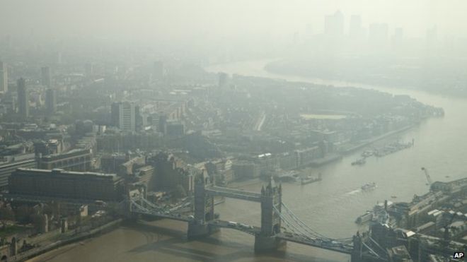
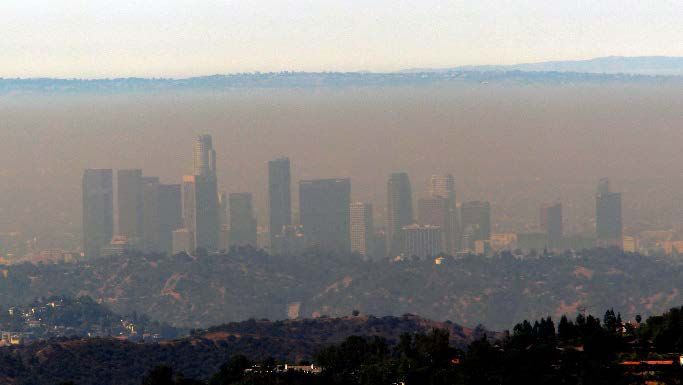
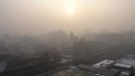
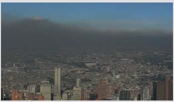
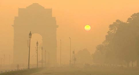
particles are incomplete combustion, automobile emission, dust and cooking. In its majority, they are
anthropogenic, with major composites being sulfates, nitrates, ammonia, carbon, lead and organic
matter. Due to their small size, PM2.5 particles are a major health hazard, because they can enter lungs
and bloodstreams of humans. They give rise to chronic damage to the respiratory- and cardiovascular
system [4, 5] and contribute to premature mortality rates [6, 7]. WHO estimates that air pollution causes
about 6.5 million premature deaths every year [8a].
Apart from devastating effects on health, PM2.5 particles are also the main cause of haze – periods with
reduced visibility occurring in urban areas all around the world [8 – 14]. Figure 1 shows examples of how
haze changes visibility in six cities. The change in visibility is related to a reduction in solar intensity and
an alteration of the spectrum reaching the ground.

 a) Delhi [21] b) Beijing [22]

 c) London [23] d) Los Angeles [24]

 e) Cairo [25] f) Bogota [26]

 Figure 1: Haze events around the world.

In this study we focus on quantifying the impact of haze on insolation levels in cities, and the reduction in
power generated by photovoltaic panels due to this effect. Until 2050, it is expected that 2.5 billion people

will live in urban areas [15]. City integrated photovoltaics (PV) offer opportunities of mitigating challenges
related to the high power demand of these growing urban areas [16, 17].
Surprising to the authors, it was difficult to assess the global capacity of PV installations in cities, based on
literature data. However, there are numerous indicators that a significant PV capacity is installed in urban
areas, and more is to come. The potential for rooftop solar PV installations in cities was estimated at
5.4 TW – 70% of the electricity demand of urban residential and commercial consumers [17a]. Only a small
fraction of this potential has been utilized so far. According to Environment America, in 2014, 6.5% of the
solar PV capacity in the United States, or 1.3G W, were installed in cities, with Los Angeles in the lead [18].
Several countries have formulated targets for rooftop installations, the most remarkable being India with
40 GW planned by 2022. China already has 22 GW of combined PV capacity installed on rooftops, and a
further boost in rooftop installations is expected in 2018 [19]. Australia had 16% of PV capacity installed
on rooftops as of 2016. Furthermore, a growing number of cities have committed themselves to achieving
100% renewable electricity or energy. Examples include San Diego and San Francisco (California),
Vancouver (Canada), Copenhagen (Denmark), Munich and Frankfurt (Germany). Other cities have
formulated targets for renewable shares of total energy – e.g. Austin (Texas) 65% by 2025 and Paris
(France) 25% by 2020 – or total electricity – e.g. Amsterdam (Netherlands), 50% by 2040, Canberra
(Australia), 90% by 2020 and Tokyo (Japan) 24% by 2024 [20]. While neither rooftop installations nor
energy targets translate directly into PV installations in cities, they are indicators for the growing amount
of solar panels installed in or near cities. There are also concrete targets for the installation of local
renewable electric capacity in cities, including Los Angeles (1.3 GW of solar PV by 2020), New York
(350 MW of PV by 2024) and San Francisco (950 MW renewables by 2020) [20].
The goal of this work is to correlate fine particulate matter concentration with a reduction of insolation
reaching solar installations in cities. We start by analyzing pollution and insolation data collected in Delhi,
India. The availability of high-quality, high-frequency insolation- and pollution data, as well as the high
levels of pollution observed in Delhi make this city a suitable test case to observe the effects of air
pollution. We apply a filtering method, introduced in [14], to find the functional relation between PM2.5
concentration and relative reduction in insolation. We then use this functional relation to estimate haze
related insolation losses in a number of cities around the globe, and to project the impact on different PV
technologies. Finally , we attempt to estimate the economic damage resulting from air pollution related
reductions in insolation.
Correlating Fine Particle Matter Concentration and Yield Losses in Delhi:
I PM2.5 Concentration and Insolation Data
The collected data used in this analysis is summarized in Figure 2. On the left hand side (a), measured
insolation of a photovoltaic installation in Paschim Vihar, Delhi is shown. Insolation was recorded between
May 2016 and November 2017 using two daily cleaned silicon sensors and a pyranometer with a frequency
of one measurement every minute. The data shown in the figure was measured with one of the silicon
sensors as this data is most representative of a silicon PV installation.
On the right hand side (b), PM2.5 data recorded at the U.S. Embassy and Consulates’ air quality monitors
in Delhi [27] is depicted. The data is recorded with a frequency of one measurement per hour and made
available through the “AirNow:” website of the Department of State [28]. The sensor is located in the
Chanakyapuri area, approximately 20 km away from the sensor measuring insolation. In the further
analysis we assume that the general trends of PM2.5 concentration are consistent over the area covering
both sites. This assumption was confirmed by measurements taken at various sites in Singapore.

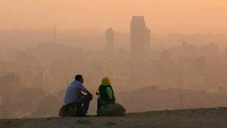
Figure 2: a) Delhi insolation measured with a silicon sensor between May 2016 and November 2017. b)
 Delhi PM2.5 concentration measured by the U.S. Embassy and Consulates’ air quality monitors [27, 28]
 c) histogram of PM2.5 concentration durations.
To classify PM2.5 concentration levels, we follow color coding for Air Quality Index (AQI) as suggested by
AirNow [29]. Note, however, that AQI and PM2.5 concentration are related but dissimilar metrics, hence
pollution levels are not directly transferrable to AQI levels as typically used. Terminology and color coding
is summarized in Table I.
Table I: PM2.5 Concentration ranges and terminology
 Concentration range
 Color Code Levels of Health Concern
 (µg/m3)
 0 – 50 Green good
 51 – 100 Yellow moderate
 101 – 150 Orange moderately unhealthy
 151 – 200 Red unhealthy
 201 – 300 Purple very unhealthy
 Above 300 Maroon hazardous

II Correlating PM2.5 Concentration and loss in Insolation
The methodology for relating PM2.5 concentration to a reduction in insolation was introduced in [14]. For
a detailed description, we refer readers to this publication, though we provide a brief summary of the
approach in the following. In [14] we suggested sorting insolation data in bins corresponding to different
levels of PM2.5 concentration, and then use humidity and clear sky filters to identify data points
representative of clear sky conditions.
We generally apply the same method here, yet with some alterations. The main difference between the
analysis presented in [14] and here is the length of time period considered. In [14] we analyzed a haze
event that took place within 18 days. Here we consider insolation data over 19 months. Over the course
of a year insolation varies via the zenith angle and the eccentricity of the Earth’s orbit around the sun [30,
31], as well as due to seasonal variations in atmospheric conditions – e.g. water content. These variations
need to be considered when analyzing correlations. For the purpose of this study, we considered data for
different moths separately. Data of different months was later combined after normalizing it to the 90
percentile of all data points collected at noon for a given month. The effect of this normalization is shown
in Figure 3 for the examples of August and December, marking the months with highest and lowest overall
insolation.

raw normalized
 August August
 December December
 1000

 insolation [W/m2]
 800

 600

 400

 200

 0
 6 9 12 15 18 6 9 12 15 18
 time of day [hour]
 Figure 3: Data measured in the months of August (yellow) and December (purple). On the left side the
 raw data is shown, on the right we show the data normalized to consider seasonal variations.

Figure 4 illustrates how we correlate PM2.5 concentration levels with a reduction in insolation. Figure 4a
shows in steps how typical daily insolation curves for different pollution conditions are obtained. The
figure on the left shows all available data points after adjustment for seasonal variations, with color coding
indicating which pollution level they belong to. In the middle, two specific conditions are selected –
moderate (50 – 100 µg/m3) and very unhealthy (200 – 300 µg/m3). The lines indicate the 80 percentile of
the ensemble for each hour and pollution level. The 80 percentile filter here fulfills the same function as
the combined humidity and clear sky filter in [14] – i.e. it identifies conditions that are representative of
a clear sky. The picture on the right, finally, shows the curves obtained for all six pollution levels. Note
that only ensembles (i.e. data sets for a specific hour and pollution level) were considered that contained
more than eight data points. This data was then used to generate Figure 4 b by considering the relative
decrease in intensity as a function of PM2.5 concentration for each hour. Note that it is possible to
correlation PM2.5 concentration and insolation reduction in a variety of different ways. We are discussing
some of them in the supporting material. The important finding is that all ways we have tried resulted in
similar functional correlations i.e. mono-exponential decays with exponents that were not significantly
different.
Also shown in Figure 4 b are previous results from [14] (cross shapes). These results are consistent with
findings presented here. The advantage of the data set acquired in Delhi is the wide range of pollution
conditions covered. Data ensembles with statistical relevance could be collected up to 375 µg/m3
concentration, a factor three more than for Singapore. One consequence of this wider range is that the
data presented here is slightly better represented by an exponential decay than by a linear function (R2 of
92% compared to 90%). Exponential decay is expected according to Lambert-Beer’s law. The fitted
exponential decay is shown as a blue line in the figure, and the functional relation is written down in
equation 1.

a) filtering… b) …and correlating

 good good
 moderate moderate
 moderate
 1200 moderate / unhealthy moderate / unhealty
 insolation [W/m2]

 unhealthy very unhealthy unhealthy
 very unhealthy very unhealthy
 hazardous
 1000 hazardous

 800

 600

 400

 200

 0
 6 9 12 15 18 6 9 12 15 18 6 9 12 15 18
 time of day [hour]
 Figure 4: a) Sketch of how data points and typical curves for a clear day under specific pollution
 conditions are obtained. The figure on the left shows the data after adjustment for seasonal variations
 with a color code depending on pollution level. In the middle figure, two conditions are highlighted and
 curves are shown that represent the 80 percentile for the data ensemble of each hour. The figure on the
 right shows the curves obtained for all pollution conditions. In b) this data is used to formulate a
 functional correlation between PM2.5 concentration and reduction of insolation by considering the
 relative reduction for each hour. Also shown are data obtained previously for Singapore [14] and a
 mono-exponential decaying fit (see equation 1).
The function describing the exponential decay in Figure 4 b is summarized in the following equation. We
will use this equation in the following to estimate how much light is lost due to air pollution. The
uncertainty given here is calculated from least mean square fitting of a mono-exponential decay. Further
details about this fit are given in the supporting material.
 ( 2.5) − 2.5
 0
 = �750±90 � (1)

III Haze related reduction in insolation and impact on a Si PV panel
The relation formulated in Equation 1 can directly be used to estimate the loss in yield due to a reduction
in insolation due to haze. Figure 5 summarizes the measured insolation for 2016 and 2017 from Figure 2
in blue, and the estimated insolation at 0 µg/m3 PM2.5 concentration in orange. The estimated curve was
obtained by adjusting the measured insolation using the PM2.5 concentration measured at the same time.

 Figure 5: Measured insolation (blue) and estimated insolation without air pollution, i.e. at a PM2.5
 concentration of 0 µg/m3 (orange).

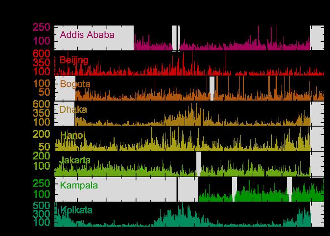
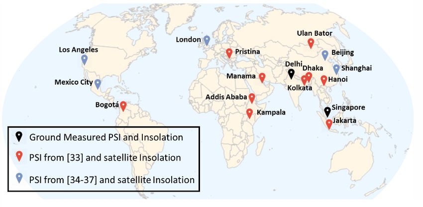
Integrating the insolation over the period of one year (May 2016 to May 2017), we obtain the annual
radiant exposure as well as the projected exposure at 0 µg/m3 PM2.5. These values are summarized in
Table II. The projected losses for Delhi are 11.5% of the annual solar energy or 200 kWh/m2. We have
also included the projected yield losses for a 20% efficient silicon PV module.
 Table II: PM2.5 Impact on insolation in Delhi over one year.
 Annual Radiant Annual yield of a 20% Si-
 Exposure [kWh/m ]2
 module [kWh/m2]
 Measured data 1570 314
 Projection 0 µg/m3 PM2.5 1770 ± 30 354 ± 6
 Ratio 88.5 ± 1.5 %
 Difference 200 ± 30 40 ± 6
Projected losses in other cities:
Using the functional relation formulated in Equation 1, we extended the assessment of loss in annual
radiant exposure to other cities. While it can be argued that the composition of haze and its optical
behavior vary from location to location [32], we found that the relation between PM2.5 concentration
and insolation we observe for Delhi also describes data from Singapore reasonably well (compare
Figure 4b). We take this as an indication that an estimate based on Delhi data can provide at least some
guidance about what losses to expect. The cities covered in this study are shown in Figure 6. We selected
cities based on availability of air quality data, known haze events and geographic distribution.

 Figure 6: Map of cities covered in this study. Black markers indicate locations for which simultaneous,
 ground-measured PM2.5 and insolation data are available. Red markers indicate locations for which
 PM2.5 data was obtained from [33], for blue markers PM2.5 data was taken from [34 - 37].

Air quality data is available from a number of sources. For the results presented in this paper, we have
used data from the AirNow Department of State (DOS) website [33]. This website provides historical data
of PM2.5 measurements for a number of cities measured at U.S. embassies and consulates around the
world. Depending on location, historical data dates back as far as 2015. For consistency reasons, we have
made use of this database wherever possible. Additional sources we used (marked in blue) come from
National or Communal centers and institutions [34 – 37]. The data obtained is summarized in Figure 7.

a) PM2.5 time series I. b) PM2.5 time series II

 c) PM2.5 histogram I d) PM2.5 histogram II

 Addis Ababa Beijing Bogota Dhaka 5.0 London 4.0 Los Angeles Manama 3.0 Mexico City
 3.0 3.0 1.0 98.4% 1.5 37.7% 95.5%
 91.7% 54.3% 98.8% 47.2% 4.0 97.9%

 1000 hours / year
 1000 hours / year

 1.0 3.0
 2.0
 2.0 2.0 3.0 1.0 4.4%
 26.1%
 2.0 1.5% 54.3%
 7.8% 24.6%
 1.2%
 0.5 2.0 2.0%
 0.5 10.6% 1.0 0.1%
 1.0 10.4% 1.0 0.1% 1.0 0.1% 0.5 6.6%
 0.4% 0.1% 7.6% 1.0
 5.0% 0.7% 0%
 0% 0.1% 0% 3.9% 1.7% 0% 0% 0% 6.5% 1.8% 0% 0% 0% 0% 0% 0% 0.5% 0.3% 0% 0%

 1.5 5.0
 Hanoi 2.0 Jakarta Kampala 1.5 Kolkata Pristina Shanghai Singapore Ulan Bator
 1.5 3.0 4.0 99.8%
 49.0% 88.9% 55.9% 2.0 71.6%
 72.2% 82.5% 51.0% 1.0
 1.5 1.0
 1.0 2.0 3.0
 1.0
 1.0 38.7% 24.0% 6.8% 25.8% 2.0 0.2%
 1.0
 19.6% 0.5 10.3%
 0.5
 16.2% 0.5 10.0% 0.5 10.4% 1.0 2.1% 9.5%
 6.4% 0.5 1.0 0% 5.1%
 1.1% 1.8% 1.0% 4.3%
 1.5% 7.9% 3.9%4.7%
 0.3% 0% 0.2% 0% 0% 0.6% 0% 1.0% 0.3% 3.0%1.6% 0% 0% 0% 4.4%
 5.2%1.6%
 0 100 200 300 400 0 100 200 300 400 0 100 200 300 400 0 100 200 300 400 500 0 100 200 300 400 0 100 200 300 400 0 100 200 300 400 0 100 200 300 400 500

 Pm2.5 [ug/m3] Pm2.5 [ug/m3]
 Figure 7: Summary of PM2.5 data obtained for cities shown in Figure 6. a) and b) show the time series
 of the data obtained from [33] and [34 -37]. Grey areas mark periods for which no data was available.
 c) and d) show the corresponding histograms of this data over the course of one year.

Note that recordings for several cities are imperfect. Examples are Bogota in May and June 2017, Moscow
in September 2017 and Richards Bay after October 2017. A dataset that does not cover a full year holds
the threat of not correctly representing seasonal influences, which results in a hard to predict uncertainty.
We have decided to still include the data for these cities, but ask the reader to consider this shortcoming
when interpreting the results.
Using the data summarized in Figure 7, and equation 1, we can estimate the relative and absolute losses
in radiant exposure. This estimate is summarized in Figure 8 and Table III. As we didn’t have access to
ground measured irradiance data for all locations, we used typical yearly irradiances, obtained from
satellite data [38] and a clear sky model [31, 39, 40]. Satellite daily average irradiance data from NASA is
available with a 1 x 1 degree resolution. Irradiance for each day of the year over the course of ten years
(2005 – 2015) was used, with the median value for each day marking the considered typical value (see
supporting material). Daily irradiance distribution was projected with the clear sky model. Corrections
with equation 1 were calculated on an hourly basis by reducing the incoming photon flux according to
PM2.5 concentration. This approach neglects contributions of clouds as well as ground reflection and
scattering. Errors can be expected if such effects occur systematically at a specific time of day, as is the
case, for example, in Singapore where morning tend to be sunnier than afternoons [41]. To benchmark

this approach, we calculated the relative losses for Delhi (shown in the last column in Table III a). The
calculated losses are 12.2 ± 0.9 %, which is consistent with the 11.5 ± 1.5 % obtained from ground based
measurements.
To project the impact on photovoltaic panels, we have included two metrics in Table III, the global tilted
irradiation for fixed systems at optimum angle (GTI) in kWh/m2, and the Photovoltaic power potential
(PVout) in kWh/kWp. Values for these metrics for the different cities were obtained from the Global Solar
Atlas [42]. Corrections and losses are calculated directly by adjusting for the relative loss (first row).
Uncertainties were obtained directly through the uncertainty in equation 1 and indirectly by varying the
beginning- and end point of the considered one year period.
 loss [%]
 relativ

 10
 5
 2500
 0
 2000
 [kWh/m2]

 1500
 GTI

 1000
 500
 [kWh/m2]

 0
 GTI loss

 200
 100
 0
 Hanoi

 Shanghai

 Ulan Bator
 Addis Ababa

 Beijing

 Bogota

 Dhaka

 Jakarta

 Kampala

 Kolkata

 Los Angeles
 London

 Manama

 Mexico City

 Pristina

 Singapore
 Figure 8: Projected relative losses in radiant exposure for the considered cities - top, as well as tabulated
 global tilted irradiation for fixed systems at optimum angle (GTI) values according to Ref [39] (bright
 colors) and corrected values (dark) - middle. Absolute loss in GTI for each city is shown in the lower part
 of the figure.

Table III a): projected relative losses in radiant exposure for the cities from Figure 7 a) and c), as well as
tabulated and corrected GTI values, GTI losses and losses in PV power potential (PVout).

 Addis
 Beijing Bogota Dhaka Hanoi Jakarta Kampala Kolkata
 Ababa
 rel. loss [%] 4.1±0.8 9.1±1.0 1.9±0.2 9.0±0.9 5.9±0.2 4.3±0.3 5.9±0.3 9.6±0.8
 GTI [kWh/m2] 2174 1634 1526 1774 1356 1721 1941 1804
 GTI corr.
 2085 1485 1497 1614 1276 1647 1826 1631
 [kWh/m2]
 GTI loss
 89±17 149±16 29±3 160±16 80±3 74±5 114±6 173±14
 [kWh/m2]
 PVout loss
 71±14 121±13 24±2 123±12 62±2 57±4 89± 132±11
 [kWh/kWp]

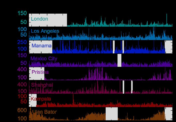
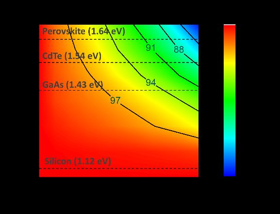
Table III b): projected relative losses in radiant exposure for the cities from Figure 7 b) and d), as well as
tabulated and corrected GTI values, GTI losses and losses in PV power potential (PVout). Delhi is included as
a reference to illustrate differences between ground based data and satellite based data.

 Los Mexico Shang- Singa- Ulan
 London Manama Pristina Delhi
 Angeles City hai pore Bator
 rel. loss [%] 2.4±0.2 2.2±0.2 7.8±0.5 3.9±0.3 3.6±0.3 8.2±079 2.0±0.2 9.2±1.0 12.2±0.9
 GTI
 1195 2267 2284 2295 1599 1428 1630 2031 1863
 [kWh/m2]
 GTI corr.
 1166 2217 2106 2205 1541 1311 1597 1864 1636
 [kWh/m2]
 GTI loss
 29±2 50±5 178±11 90±7 58±5 117±10 33±3 167±20 227±17
 [kWh/m2]
 PVout loss
 24±2 39±4 137±9 71±5 47±4 94±8 25±3 144±18 174±13
 [kWh/kWp]

Projection to other PV technologies:
Losses in radiant exposure are not distributed uniformly across the solar spectrum. Data acquired in
Singapore shows that shorter wavelengths are more affected, which is in line with expectations from basic
scattering theory [43]. Hence, solar cells with a larger band gap should be more strongly affected than
silicon. We projected the impact on other PV technologies by considering changes in absorption up to the
band gap of the specific solar cell technology as a function of PM 2.5 concentration. Four band gaps were
considered: silicon (1.12 eV) as baseline, GaAs (1.43 eV), CdTe (1.54 eV) and a material from the
perovskite family (1.64 eV) [44, 45] and four locations: Delhi, Beijing, Hanoi and Mexico City. The results
of this exercise are shown in Figure 9 and Table IV. Compared to silicon, losses are projected to be
increased by 23% for GaAs, 33% for CdTe and 42% for perovskites.

a) Spectrum changes with PM25 b) PM2.5 concentration vs APE

 2.0 1.96
 PM25 = 25
 spectral irradiance

 PM25 = 50
 PM25 = 75 1.92
 [W/(m2 nm)]

 1.5 PM25 = 125

 APE [eV]
 PM25 = 200 1.88
 PM25 = 275
 1.0
 1.84

 0.5 1.80

 1.76
 0 0 100 200 300
 400 600 800 1000
 PM2.5 concentration
 wavelength[nm]
 c) projected impact on photon flux d) linear approximation of flux attenuation

 e) projection for cities and technologies Figure 9: Effect of fine particulate matter on
 different PV technologies. a) Shows on examples
 20
 Si
 how the solar spectrum is affected by different
 GaAs PM2.5 concentrations. b) Summarizes the relation
 between PM2.5 concentration and average
 relative loss [%]

 15 CdTe
 Perovskite
 photon energy. The line is a guide to the eye. c)
 10
 Projects the impact of PM2.5 concentration on the
 absorbed photon flux for absorbers with different
 band gaps. d) Illustrates the reduction in photon
 5
 flux per PM2.5 concentration and band gap. In e)
 this relation is used to project the PM2.5 induced
 0
 Delhi Beijing Hanoi Mexico City
 losses onto different PV technologies.

Table IV): projected relative losses in absorbed photon flux for different PV technologies and four
exemplary locations (compare Figure 9e)

 Silicon (1.12 eV) GaAs (1.43 eV) CdTe (1.54 eV) Perovskite (1.64 eV)
 Delhi 12.2 15.0 16.1 17.2
 Beijing 9.1 11.2 12.0 12.8
 Hanoi 5.9 7.3 7.8 8.3
 Mexico City 3.9 4.8 5.2 5.5

Economic considerations:
Using these numbers and Table 3, we can estimate the loss in revenue to PV installers and operators. The
average price for residential electricity in Delhi in January 2017 was 12.2 ct/kWh (8.07 ₹/kWh) [46]. The
estimated loss in PV power output is 174 kWh/kWp annually, resulting in a loss of 21.23 $US/kWp each
year – or 12% relative. Given the targets formulated by the Indian government, rooftop installations in
Delhi can be expected to be in the GW range, which would put the annual damage to economy above 20
million dollars. Similarly, the estimated damage in Kolkata is 16 million dollars per GW.
In China, residential power prices are given as 7.9 ct/kWh (0.495 yuan/kWh) in Beijing and 9.1 ct/kWh
(0.571 yuan/kWh) in Shanghai [47]. The estimated loss in annual revenue here is 10 million dollars per
GW installed for Beijing and 9 million dollars per GW installed in Shanghai.
However, even for cities with better air quality like Los Angeles air pollution causes notable economic
damage. Average electricity costs for household electricity in Los Angeles in February 2018 were
18.4 ct/kWh [48] and 11.7 ct/kWh [49] for industry. Using the installation target of 1.3 GW by 2020,
annual losses are between 5.9 and 9.3 million dollar.
Discussion:
I Comparison to literature
Aerosols affect how sunlight passes through the atmosphere. This has been known since Tyndall observed
that blue light is scattered more strongly than red light when passing through a clear fluid holding small
particles [50]. And already Tyndall was concerned with the question how small particles that affect the
passage of light would influence health. “Nor is the disgust abolished by the reflection that, although we
do not see the nastiness, we are churning it in our lungs every hour and minute of our lives.” He writes in
an article in Nature in 1870 [51]. As discussed earlier, the concerns were well founded and numerous
studies have confirmed the detrimental effects of haze on health – even if they are different than what
Tyndall imagined.
Attempts to quantify the effect of aerosol particles on solar irradiance have also been made. A study by
Husar et al. [52] and Guyemard et al. [53] looked at the effect on solar irradiation caused by two intense
dust storms in the Gobi dessert. When reaching the United States, the dust clouds resulted in a 30%
reduction in direct normal solar radiation, and a 3.8% to 5.1% reduction in global horizontal irradiance
(GHI). The increase in air pollution in China has triggered a number of studies that investigate the
correlation between aerosols and solar irradiance. Li et al. [54] correlated satellite measured air pollution
data and solar photovoltaic resource in China. They found that the combined aerosol optical depth of all
particles reduced solar irradiance by 20% - 35%. Note that this study considers all aerosols in the
atmospheric column, whereas results presented here only considers fine particulate matter.
We note that there is an increasing awareness of the role of air pollution on PV power generation, yet
quantifying the correlation between anthropogenic air pollution and a reduction in solar resource using
ground-based measurements seems to be lacking. This study is an attempt to provide the missing
information.
II Air pollution and soiling
The work presented here only considers the reduction in solar resource due to light extinction caused by
PM2.5 particles in the lower atmosphere. Air pollution causes an additional reduction in PV performance

by dust accumulation on the solar panel. A discussion about the impact of different types of aerosols is
given in [55], a general overview of the field is given in [56].
III Threats and Opportunities
Solar Photovoltaics are both affected by air pollution and could provide a way to reduce it. One example:
approximately 2.8 billion people cook with solid fuels, rendering cooking one of the prevalent sources of
fine particulate matter in India, Pakistan and Southern Africa [57]. Solar or PV powered cookers [58, 59]
provide an almost pollution free alternative, and generally solar energy is thought to play an important
role in improving air quality [50, 61]. However, air pollution induced scattering and extinction of light
reduces the available solar resource and increase the fraction of diffuse light. These effects, if not
considered correctly, can make solar powered application underperform and become unreliable [62, 63]
- a threat to wide-spread adoption.
Policymakers in many regions are now acting to address air pollution issues. Dedicated Policies and the
use or renewable energy sources can improve air quality, as many cities around the world have
demonstrated. Notable examples include Vittoria-Gasteiz (Spain), Montréal (Canada), Lisbon (Portugal),
Medellín (Colombia) and Seoul (South Korea), which managed to reduce air pollution between 28% and
63% [64]. China has drawn up an aggressive “battle plan” against smog that seems to have positive effects
in cities like Beijing and Tianjin [65, 66]. In a previous action plan (2013 to 2017), a 25% reduction in PM2.5
concentration was targeted. A reduction in PM2.5 concentration is visible in Figure 7b for Beijing and
Shanghai in the second half of 2017. Also India has formulated targets on reducing air pollution [67],
though recent news do not indicate significant improvements in air quality [68].
Summary and Conclusions:
Urban haze is a threat with a multifaceted nature. It consists largely of anthropogenic fine particulate
matter (PM2.5) generated to a large extent by incomplete combustion processes. Haze is a serious health
hazard as it can penetrate deeply into the lungs and cause chronic damage to the respiratory system. Haze
also affects the transition of light through the lower atmosphere, reducing the overall intensity of light
reaching the ground and increasing the diffuse fraction.

Relation between PM2.5 concentration and insolation:

We analyze the relation between PM2.5 concentration and the loss in solar irradiance received by flat-
panel silicon photovoltaic installations. Using long-term field data with high time-resolution from Delhi
and Singapore, we introduce a functional relation that describes the measured data up until PM2.5
concentrations of 400 µg/m3 and takes the form of a mono-exponential decay:
 ( 2.5) − 2.5
 = � �
 0 750 ± 90
Estimating insolation losses in Delhi:

Using this function relation, we project how much insolation Delhi would have received if no air pollution
was present for the period between May 2016 and November 2017. We find that within a one-year period
insolation was reduced by 11.5 ± 1.5 % or 200 kWh/m2 (from 1770 kWh/m2 to 1570 kWh/m2) by fine
particulate matter.

Projection to other cities:

Using available air quality data and satellite measured insolation, we extended this analysis to 16 more
cities in Africa (Addis Ababa, Kampala), the Americas (Bogota, Los Angeles, Mexico City), Asia (Beijing,
Dhaka, Hanoi, Jakarta, Kolkata, Manama, Shanghai, Singapore, Ulan Bator) and Europe (London, Pristina).
Repeating the analysis for Delhi, we found that using satellite data for a typical year (2006 – 2015) resulted
in estimated losses that are consistent with those obtained from analyzing field measurements (12.2 ±
0.9%). Estimated losses range from 2.0% relative or 29 kWh/m2 per year (Singapore) to 9.1% relative or
149 kWh/m2 per year (Beijing). We also projected losses in PV power potential and obtained values ranging
from 24 kWh/kWp (London) to 144 kWh/kWp (Ulan Bator).

Projection to other PV technologies:

Using spectrum measurements from Singapore, we also projected how haze affects different PV
technologies. Haze affects blue light stronger than red light, resulting in PV materials with larger band
gaps being more affected than silicon. Adjusting for additional current losses we predict that losses
increase by 23% relative for GaAs, 33% for CdTe and 42% for perovskites (at 1.64 eV band gap) compared
to silicon.

Economic implications

Reduced insolation results in lost revenues for system operators and investors in PV systems. Given the
aggressive installation goals for many countries and communities, installations in urban areas in the order
of GW can be expected. For installations of this magnitude and current electricity prices, projected annual
losses in revenue for Delhi could well exceed 20 million dollars, or 12% of total revenue. Similarly,
projected losses for GW installations would suffer annual losses of 16 million dollars in Kolkata and around
10 million dollars in Beijing and Shanghai. In Los Angeles with a target capacity of 1.3 GW of installed solar
by 2020, projected annual economic losses are between 6 and 9 million dollars. These numbers indicate
that global losses in revenue could easily amount to hundreds of millions, if not billions of dollars annually.
An additional factor is that the reduced insolation and changed character of sunlight (more diffuse light),
if not accounted for correctly, will affect the reliability of PV powered systems with a hard to quantify
reduction in adoption.

Acknowledgments:
The authors thank Liu Zhe for help with Chinese websites and texts. This work was financially supported
by funding from Singapore's National Research Foundation through the Singapore MIT Alliance for
Research and Technology's “Low energy electronic systems (SMART - LEES) IRG” and by the DOE-NSF ERF
for Quantum Energy and Sustainable Solar Technologies (QESST).

References:
[1] J. Vidal, “Air pollution rising at an 'alarming rate' in world's cities”, The Guardian, 11 May 2016,
 https://www.theguardian.com/environment/2016/may/12/air-pollution-rising-at-an-alarming-rate-in-worlds-cities
[2] World Health Organization. Ambient air pollution: A global assessment of exposure and burden of disease. World Health
 Organization. 1 – 131 (2016).
[3] Hannah Ritchie and Max Roser - "Air Pollution". Published online at OurWorldInData.org. Retrieved from:
 'https://ourworldindata.org/air-pollution' [Online Resource] (2017).
[4] K. Kornei, “Here are some of the world’s worst cities for air quality”, Science (2017), doi:10.1126/science.aal0942,
 http://www.sciencemag.org/news/2017/03/here-are-some-world-s-worst-cities-air-quality
[5] EPA, Overview of Particle Air Pollution, Presented at the Air Quality Communication Workshop, San Salvador (2012).

The impact of pollution on health and mortality is well documented. These are just two prominent of many good examples:
[6] J. Lelieveld, J. S. Evans, M. Fnais, D. Giannadaki & A. Pozzer, “The contribution of outdoor air pollution sources to
 premature mortality on a global scale”, Nature 525 (2015), 367 – 371.
[7] Beelen, R. et al. Effects of long-term exposure to air pollution on natural-cause mortality: an analysis of 22 European
 cohorts within the multicentre ESCAPE project. Lancet 383 (2014), 785–795.
There is a range of literature on haze in different locations, especially China. Examples are:
[8] D. Mishra, P. Goyal, A. Upadhyay, “Artificial intelligence based approach to forecast PM2.5 during haze episodes: A case
 study of Delhi, India”, Atmospheric Environment, 102 (2015), 239 – 248.
[8a] http://www.who.int/airpollution/en/
[9] R. Gottlieb and S. Ng, “Global Cities, Urban Environments in Los Angeles, Hong Kong, and China”, MIT Press, May 19,
 2017.
[10] M. Iftikhar, K. Alam, A. Sorooshian, W. A. Syed, S. Bibi, H. Bibi, “Contrasting aerosol optical and radiative properties
 between dust and urban haze episodes in megacities of Pakistan”, Atmospheric Environment, 173 (2018), 157 – 172.
[11] Zhang R. et al. (2017) Overview of Persistent Haze Events in China. In: Bouarar I., Wang X., Brasseur G. (eds) Air Pollution
 in Eastern Asia: An Integrated Perspective. ISSI Scientific Report Series, vol 16. Springer, Cham.
[12] G. Wang, et al., Persistent sulfate formation from London Fog to Chinese haze, PNAS 113 (2016), 13630 – 13635.
[13] H. Liu et al., The Impact of Haze on Performance Ratio and Short-Circuit Current of PV Systems in Singapore, IEEE JPV 4
 (2014), 1585-1592.
[14] A. Nobre et al., On the impact of haze on the yield of photovoltaic systems in Singapore, Renewable Energy 89 (2016),
 389 – 400.
[15] United Nations Department of Economic and Social Affairs, Population Division, World Urbanization Prospects: The 2014
 Revision, CD-ROM Edition (United Nations, 2014).
[16] D. M. Kammen, D. A. Sunter, City-integrated renewable energy for urban sustainability, Science 352 (2016), 922 – 927.
[17] S. Castellanos, D. A. Sunter, and D. M. Kammen, „Rooftop solar photovoltaic potential in cities: how scalable are
 assessment approaches?“, Environ. Res. Lett. 12 (2017) 125005.
[17a] IEA, Energy Technology Perspective 2016, Annex H – Rooftop Solar PV Potential in Cities.
 https://www.iea.org/etp/etp2016/annexes/
[18] J. Burr, L. Hallock, R. Sargent, “Shining Cities – Harnessing the Benefits of Solar Energy in America”, EA Report 2015.
[19] PVMagazine, “Rooftop PV key driver of 2017 installation forecast hike in China”, Novemer 23rd 2017, https://www.pv-
 magazine.com/2017/11/23/driving-forces-behind-chinas-2017-solar-boom/
[20] REN21, Renewables 2016, Global Status Report, Renewable Energy Policy Network (2016), http://www.ren21.net/wp-
 content/uploads/2016/06/GSR_2016_Full_Report.pdf
[21] https://www.ecowatch.com/top-weather-events-2016-2180215649.html
[22] http://www.climatechangenews.com/2017/03/23/melting-arctic-worsens-beijings-pollution-haze-study-finds/
[23] http://www.bbc.com/news/uk-32233922
[24] https://www.nbcnews.com/science/environment/cough-cough-climate-change-may-worsen-air-pollution-n136986
[25] https://moderndiplomacy.eu/2017/12/21/cairos-bad-breath/
[26] https://sds-was.aemet.es/events/4th-colombian-meeting-and-international-conference-on-air-quality-and-public-
 health
[27] Information about the Air Quality data measured by the U.S. Embassy and Consulates in India is provided here:
 https://in.usembassy.gov/embassy-consulates/new-delhi/air-quality-data/
[28] Datasets for Delhi can be downloaded here:
 https://www.airnow.gov/index.cfm?action=airnow.global_summary#India$New_Delhi
[29] https://airnow.gov/index.cfm?action=aqibasics.aqi
[30] R. G. Allen, Environmental, and E. Water Resources Institute. Task Committee on Standardization of Reference, The
 ASCE standardized reference evapotranspiration equation, Reston, Va.: American Society of Civil Engineering (2005).
[31] M. J. Reno, C. W. Hansen, J. S. Stein, Global Horizontal Irradiance Clear Sky Models: Implementation and Analysis, Sandia
 Report, SAND2012-2398, Sandia National Laboratories (2012)
[32] G. Snider et al., “Variation in global chemical composition of PM2.5: emerging results from SPARTAN”, Atmos. Chem.
 Phys., 16 (2016), 9629–9653.
[33] The data for a number of cities is provided here: https://airnow.gov/index.cfm?action=airnow.global_summary
 (compare Ref [29])
[34] Data for Beijing and Shanghai was obtained from the China National Environmental Monitoring Centre (CNEMC),
 http://www.cnemc.cn/
[35] Data for London was obtained from the London Air Quality Network (LAQN),
 http://www.londonair.org.uk/LondonAir/General/about.aspx
[36] Data for Mexico City was obtained from Red Automática de Monitoreo Atmosférico (RAMA) of the city of Mexico,
 http://www.aire.df.gob.mx/default.php?opc=%27aKBh%27

[37] Data for Los Angeles was obtained from the California Air Resource Board, https://ww2.arb.ca.gov/
[38] Irradiance data is obtained from NASA’s Clouds and the Earth’s Radiant Energy System (CERES) website,
 https://ceres.larc.nasa.gov/
[39] V. Badescu, "Verification of some very simple clear and cloudy sky models to evaluate global solar irradiance," Solar
 Energy, vol. 61, pp. 251-264, Oct 1997.
[40] R. G. Allen, Environmental, and E. Water Resources institute . Task Committee on Standardization of Reference, The
 ASCE standardized reference evapotranspiration equation. Reston, Va.: American Society of Civil Engineers, 2005.
[41] Y. S. Khoo, A. Nobre, R. Malhotra, D. Yang, R. Rüther, T. Reindl, A. Aberle, “Optimal Orientation and Tilt Angle for
 Maximizing in-Plane Solar Irradiation for PV Applications in Singapore”, IEEE Journal of Photovoltaics, 4 (2014), 647 –
 653.
[42] http://globalsolaratlas.info/
[43] J. Strutt, "On the transmission of light through an atmosphere containing small particles in suspension, and on the origin
 of the blue of the sky," Philosophical Magazine, 5 (1899), 375–394.
[44] I. M. Peters, L. Haohui, T. Reindl, T. Buonassisi, Global Prediction of Photovoltaic Field Performance Differences Using
 Open-Source Satellite Data, Joule, 2 (2018), 307 – 322.
[45] I.M. Peters, T. Buonassisi, Energy Yield Limits for Single Junction Solar Cells, Joule (2018), published online.
[46] R. Toniga, Delhi’s Household Electricity Subsidies: Highly Generous but Inefficient? Brookings India IMPACT Series No.
 042017. April 2017
[47] N. Zhou, Lawrence Berkeley National Laboratory China Energy Group, KEY CHINA ENERGY STATISTICS 2016, (2017).
 https://china.lbl.gov/sites/default/files/misc/ced-9-2017-final.pdf
[48] United States Department of Labor, Bureau of Labor Statistics, Average Energy Prices, Los Angeles-Long Beach-Anaheim
 – February 2018, https://www.bls.gov/regions/west/news-release/averageenergyprices_losangeles.htm.
[49] https://www.electricitylocal.com/states/california/los-angeles/
[50] J. Tyndall, “On Radiation through the Earth’s Atmosphere”, Proceedings of the Royal Institution, Jan. 23 (1863).
[51] J. Tyndall, “On haze and dust”, Nature (1870), 339 – 342.
[52] R.B. Husa et al., „Asian dust events of April 1998”, Journal of Geophysical Research, 106 (2001), 18317 – 18330.
[53] C. A. Gueymard, C. N. S. Laulainen, J. K. Vaughan, and F. E. Vignola, China’s dust affects solar resource in the U.S.: A case
 study, SOLAR 2000, paper presented at the ASES Annual Conference, U.S. Dep. of Energy, Madison, Wisc., June 16 –21,
 (2000).
[54] X. Li, F. Wagner, W. Peng, J. Wang. D. Mauzerall, “Reduction of solar photovoltaic resources due to air pollution in
 China”,PNAS 114 (2017), 11867 -11872.
[55] L. Micheli, M. Muller, S. Kurtz, Determining the effects of environment and atmospheric parameters on PV field
 performance, Proceedings of the 43rd IEEE PVSC, Portland OR (2016).
[56] S. C. S. Costa, A. S. A. C. Diniz, L. L.Kazmerski, Solar energy dust and soiling R&D progress: Literature review update for
 2016, Renewable and Sustainable Energy Reviews, 82(2018), 2504-2536.
[57] Z. A. Chafe, M. Brauer, Z. Klimont, R. Van Dingenen, S. Mehta, S. Rao, K. Riahi, F. Dentener,and K. R. Smith, Household
 Cooking with Solid Fuels Contributes to Ambient PM2.5 Air Pollution and the Burden of Disease, Environmental Health
 Perspectives, 122 (2014), 1314 – 1320.
[58] S. D. Pohekar, M. Ramachandran, Multi-criteria evaluation of cooking energy alternatives for promoting parabolic solar
 cooker in India, Renewable Energy 9 (2004), 1449 – 1460.
[59] S. B. Joshi, A. R. Jani, Design, development and testing of a small scale hybrid solar cooker, Solar Energy 122 (2015), 148
 -155.
[60] Z. Peidong, Y. Yanli, S. Jin, Z. Yonghong, W. Lisheng, L.Xinrong, Opportunities and challenges for renewable energy policy
 in China, Renewable and Sustainable Energy Reviews, 13 (2009), 439 – 449.
[61] M. Z. Jacobsen, Review of solutions to global warming, air pollution, and energy security, Energy & Environmental
 Science, 2 (2009), 148 – 173.
[62] S. Watson, D. Bian, N. Sahraei, A. G. Winter, T. Buonassisi, I. M. Peters, Advantages of operation flexibility and load sizing
 for PV-powered system design, Solar Energy 162 (2018), 132-139.
[63] N. Sahraei, S. M. Watson, A. Pennes, I. M. Peters, T. Buonassisi, Design approach for solar cell and battery of a persistent
 solar powered GPS tracker, Japanese Journal of Applied Physics 56 (2017), 08ME01.
[64] http://talkofthecities.iclei.org/how-these-five-global-cities-have-improved-their-air-quality/
[65] https://www.reuters.com/article/us-china-pollution/china-puts-finishing-touches-to-three-year-smog-crackdown-plan-
 idUSKBN1FK095
[66] https://phys.org/news/2018-01-china-air-quality.html
[67] http://www.who.int/bulletin/volumes/94/7/16-020716/en/
[68] https://www.nytimes.com/2017/12/08/world/asia/india-pollution-modi.html

Supporting Material:
I Typical insolation from satellite data
 a) Addis Ababa b) Beijing c) Bogota d) Dhaka
 insolation W m2

 insolation W m2

 insolation W m2
 insolation W m2
 300 300 300 300
 200 200 200 200
 100 100 100 100
 0 0 0 0
 0 100 200 300 0 100 200 300 0 100 200 300 0 100 200 300
 day day day day
 e) Hanoi f) Jakarta g) Kampala h) Kolkata
 insolation W m2

 insolation W m2

 insolation W m2

 insolation W m2
 300 300 300 300
 200 200 200 200
 100 100 100 100
 0 0 0 0
 0 100 200 300 0 100 200 300 0 100 200 300 0 100 200 300
 day day day day
 i) London j) Los Angeles k) Manama l) Mexico City

 insolation W m2
 insolation W m2

 insolation W m2
insolation W m2

 300 300 300 300
 200 200 200 200
 100 100 100 100

 0 0 0 0
 0 100 200 300 0 100 200 300 0 100 200 300 0 100 200 300
 day day day day
 m) Pristina n) Shanghai o) Singapore p) Ulan Bator
 insolation W m2
 insolation W m2
insolation W m2

 insolation W m2
 300 300 300
 300
 200 200 200
 200
 100 100 100 100
 0 0 0 0
 0 100 200 300 0 100 200 300 0 100 200 300 0 100 200 300
 day day day day
 Figure S1: Median insolation based on 10 year insolation data from NASA for each day of the year and the 16
 cities considered in this study (red). This data was used to estimate insolation losses due to fine particulate
 matter. Also shown is the insolation data for one year (2014) for comparison. Note that all given values are
 average insolation values for one day.

II Correlating PM2.5 and Insolation

 900
 uncertainty from regression

 decay factor
 800
 80percentile

 Median / Fit
 20percentile
 700

 600
 7 point fit
 8 point fit
 500
 72 74 76 78 80 82 84 86 88 90 92
 humidty cutoff [%]
 Figure S2: Monte-Carlo analysis of the exponential decay factor for varying conditions of data sorting
 and analysis.

 There is a choice of parameters when it comes to sorting the insolation data for different PM2.5
 concentration conditions, which affects the exponential decay factor in equation 1. In Figure S2 we
 show a Monte Carlo analysis of how the decay factor varies when several of these factors are varied
 randomly. The x-axis of the figure corresponds to the humidity-cutoff factor. Humidity is used as an
 indication for rainy days. As can be seen, no results are shown for cutoff factors beyond 90%. Including
 days with very high humidity results in a failure of the fitting routine. On the other hand, reducing the
 cutoff factor to below 78% eliminates so many data points that fitting up until a PM2.5 concentration
 of 400 µg/m3 becomes impossible. This is indicated by the shape of the points in Figure S2. Rectangular
 shapes indicate that 8 points (i.e. concentration until 400 µg/m3) were considered, whereas round
 shapes indicate that 7 points (until 350 µg/m3) were considered. Overall, however, little dependence is
 found on the humidity cutoff. The value used in the analysis is 80%.
 A stronger dependence can be seen on the percentile that was used to define clear-sky conditions. This
 filter is used to obtain a typical daily curve from the set of points at each hour and each PM2.5
 concentration conditions (compare Figure 3a). The default value here was 0.8. Blue colors indicate a
 smaller value, red values a larger value. The goal here was to use a factor that was as large as possible
 without being influenced by outliers. As can be seen, the median value (solid line) is very close to an
 upper boundary beyond which only lie very few points. The default value was chose such that the result
 coincides with the median value. Other factors did not show a significant impact on the result.
 Overall, we find that the vast majority of all points (>95%) lies within the range that the regression gave
 as confidence interval when fitting the linear decay for the chosen conditions. Hence, we used this
 confidence interval in the analysis.