Using TROPOspheric Monitoring Instrument (TROPOMI) measurements and Weather Research and Forecasting (WRF) CO modelling to understand the ...
←
→
Page content transcription
If your browser does not render page correctly, please read the page content below
Atmos. Chem. Phys., 21, 5393–5414, 2021
https://doi.org/10.5194/acp-21-5393-2021
© Author(s) 2021. This work is distributed under
the Creative Commons Attribution 4.0 License.

Using TROPOspheric Monitoring Instrument (TROPOMI)
measurements and Weather Research and Forecasting (WRF) CO
modelling to understand the contribution of meteorology and
emissions to an extreme air pollution event in India
Ashique Vellalassery1 , Dhanyalekshmi Pillai1,4 , Julia Marshall2,a , Christoph Gerbig2 , Michael Buchwitz3 ,
Oliver Schneising3 , and Aparnna Ravi1,4
1 Indian  Institute of Science Education and Research (IISERB) Bhopal, Bhopal, India
2 Max   Planck Institute for Biogeochemistry, Jena, Germany
3 Institute of Environmental Physics (IUP), University of Bremen, Bremen, Germany
4 Max Planck Partner Group (IISERB), Max Planck Society, Munich, Germany
a now at: Deutsches Zentrum für Luft- und Raumfahrt, Institut für Physik der Atmosphäre, Oberpfaffenhofen, Germany

Correspondence: Dhanyalekshmi Pillai (dhanya@iiserb.ac.in, kdhanya@bgc-jena.mpg.de)

Received: 4 October 2020 – Discussion started: 26 October 2020
Revised: 2 February 2021 – Accepted: 2 March 2021 – Published: 8 April 2021

Abstract. Several ambient air quality records corroborate         model agreement with a correlation coefficient ranging from
the severe and persistent degradation of air quality over         0.41 to 0.60 for measurement locations across the IGP. We
northern India during the winter months, with evidence of         find that daily satellite observations can provide a first-order
a continued, increasing trend of pollution across the Indo-       inference of the CO transport pathways during the enhanced
Gangetic Plain (IGP) over the past decade. A combination          burning period, and this transport pattern is reproduced well
of atmospheric dynamics and uncertain emissions, includ-          in the model. By using the observations and employing the
ing the post-monsoon agricultural stubble burning, make it        model at a comparable resolution, we confirm the signifi-
challenging to resolve the role of each individual factor. Here   cant role of atmospheric dynamics and residential, industrial,
we demonstrate the potential use of an atmospheric transport      and commercial emissions in the production of the exorbitant
model, the Weather Research and Forecasting model cou-            level of air pollutants in northern India. We find that biomass
pled with chemistry (WRF–Chem) to identify and quantify           burning plays only a minimal role in both column and surface
the role of transport mechanisms and emissions on the oc-         enhancements of CO, except for the state of Punjab during
currence of the pollution events. The investigation is based      the high pollution episodes. While the model reproduces ob-
on the use of carbon monoxide (CO) observations from              servations reasonably well, a better understanding of the fac-
the TROPOspheric Monitoring Instrument (TROPOMI) on               tors controlling the model uncertainties is essential for relat-
board the Sentinel-5 Precursor satellite and the surface mea-     ing the observed concentrations to the underlying emissions.
surement network, as well as the WRF–Chem simulations,            Overall, our study emphasizes the importance of undertaking
to investigate the factors contributing to CO enhancement         rigorous policy measures, mainly focusing on reducing res-
over India during November 2018. We show that the simu-           idential, commercial, and industrial emissions in addition to
lated column-averaged dry air mole fraction (XCO) is largely      actions already underway in the agricultural sectors.
consistent with TROPOMI observations, with a spatial cor-
relation coefficient of 0.87. The surface-level CO concen-
trations show larger sensitivities to boundary layer dynam-
ics, wind speed, and diverging source regions, leading to a
complex concentration pattern and reducing the observation-

Published by Copernicus Publications on behalf of the European Geosciences Union.

5394                                  A. Vellalassery et al.: Understanding India’s air pollution with TROPOMI and WRF

1   Introduction                                                    of the top 20 most polluted cities in the world are located
                                                                    in the IGP region, which also includes India’s capital re-
Biomass burning (BB) has been recognized as the second-             gion, Delhi. Earlier studies and reports attributed this to sev-
largest source of radiatively and chemically active trace gases     eral reasons but mainly to crop residue burning over Pun-
(e.g. carbon monoxide – CO; carbon dioxide – CO2 ; and sul-         jab and Haryana, the two adjoining states of India’s capital
fur dioxide – SO2 ) and aerosols (e.g. particulate matter –         city of Delhi (Girach and Nair, 2014; Gupta et al., 2004;
PM10 and PM2.5 ) in the global atmosphere, which has sig-           Sidhu et al., 1998). However, the contributions from different
nificant implications for climatic change and human health          source sectors and source regions on Delhi’s pollution levels
(Andreae, 2001; Bond, 2004; Crutzen and Andreae, 1990;              still remain highly uncertain, which hinders the implemen-
Guenther et al., 2006; Kaiser et al., 2012; van der Werf et al.,    tation of definitive measures to address pollution events. A
2017). According to previous reports, BB alone accounts for         recent study reported a general lack of reliable data and re-
59 % of black carbon (BC) emissions, one-third to one-half          search efforts on biomass-burning-related issues on environ-
of global carbon monoxide (CO), and 20 % of nitrogen oxide          ment and human health (Yadav et al., 2017). Since agricul-
(NOx ) emissions (Akagi et al., 2011; Andreae, 2019). Based         tural stubble burning is a practice prohibited by law in India,
on the model estimates of Ward et al. (2012), in the absence        official surveys conducted to estimate the extent of fire emis-
of fire-related emissions, there would be a reduction of about      sion are not reliable. There is, therefore, a critical need to
40 ppm (parts per million) CO2 from the current atmospheric         improve the current knowledge base to help to make future
concentration level, indicating the importance of fire activi-      policies and implement mitigation strategies.
ties for the global carbon budget.                                     Kaiser et al. (2012) demonstrated an approach for the
   In India, emissions from open biomass burning include            calculation of biomass burning emissions by assimilat-
significant contributions from agricultural crop residue burn-      ing satellite-based fire radiative power (FRP) observations.
ing, in addition to forest and grassland fires, and play an         Along with FRP data, this approach derives the combustion
essential role in terms of releasing total carbon content to        rate and trace gas emissions subsequently, with land-cover-
the atmosphere. Agricultural stubble burning during the post-       specific conversion factors and emission factors compiled
harvesting period is one of the main kinds of biomass burning       through literature surveys. While the FRP-based approach
practices used in India to clear the land to make it suitable for   has a clear advantage of enhancing accuracy compared to
the next crop (Tai-Yi, 2012; Zha et al., 2013). According to        other inventory-based data sets, such as the Global Fire Emis-
previous estimates, crop waste open burning, which includes         sion Database (GFED), several studies have indicated inac-
its use in residential heating and cooking, is responsible for      curacies in the FRP-derived biomass burning products due to
78 %–83 % (116–289 Tg yr−1 ) of the total biomass burned in         instrument limitations and usage of conversion factors (Cus-
India during the year 2001, while rest of the contributions         worth et al., 2018; Dekker et al., 2019; Huijnen et al., 2016;
are from forest fires (Venkataraman et al., 2006). As per the       Kaiser et al., 2012; Mota and Wooster, 2018). The recent
previous studies, the primary crop residues generated in In-        availability of greenhouse gas satellite observations with un-
dia are rice straw (112 Mt), wheat straw (109.9 Mt), rice husk      precedented data density at high spatial and temporal reso-
(22.4 Mt), sugarcane tops (97.8 Mt), and bagasse (101.3 Mt),        lution paves the more direct way for a detailed study on the
the major part of which is burnt in the open air (Lasko and         origin, distribution, and extent of trace gas levels over a vast
Vadrevu, 2018). Most of these burning activities are found          domain on a monthly to daily basis. Carbon monoxide (CO)
over the northern part of India along the foothills of the Hi-      is one of the major gases emitted from biomass burning and
malayas known as the Indo-Gangetic Plains (hereafter called         incomplete fossil fuel combustion. The major sink of CO is
the IGP). The IGP is a highly populated and very important          its reaction with the hydroxyl radical (OH) to form CO2 and
agro-eco region in South Asia, which includes the states of         precursor tropospheric ozone. The lifetime of CO in the at-
Punjab, Haryana, Bihar, Uttar Pradesh, and West Bengal. The         mosphere is between several weeks and several months and
region occupies nearly 20 % of the total geographical area of       varies with the location and season, depending on the oxidiz-
India and contributes about 42 % to India’s total grain pro-        ing capacity of the environment (Jaffe, 1968). Compared to
duction (Tripathi et al., 2007). Based on VIIRS (Visible In-        CO2 and methane (CH4 ), the short lifetime of CO makes it
frared Imaging Radiometer Suite) thermal anomalies, a re-           easier to detect from the background concentration level, and
cent study has estimated burnt crop residues of 20.4 Mt and         thus, it can be a good tracer of pollution transport (Dekker et
9.6 Mt in Punjab and Haryana for the agricultural year 2017–        al., 2017). Therefore, CO can be used as a proxy for the an-
2018 in which most of the residue burnt (>90 %) at the field        thropogenic emissions of other pollutants, for example, emis-
was from rice and wheat crops (Singh et al., 2020).                 sions of important greenhouse gases (GHGs) such as CO2
   Episodes of pollution events are a major concern in the          (Gamnitzer et al., 2006).
IGP region, which worsen during post-monsoon and win-                  The TROPOspheric Monitoring Instrument (TROPOMI),
ter seasons (Cusworth et al., 2018; Dekker et al., 2019;            on board the Sentinel-5 Precursor satellite, has been mea-
Girach and Nair, 2014). According to the World Air Qual-            suring various trace gases, including CO, since November
ity Report 2019 based on ambient PM2.5 concentration, 14            2017 (Landgraf et al., 2016; Borsdorff, 2018; Borsdorff et al.,

Atmos. Chem. Phys., 21, 5393–5414, 2021                                               https://doi.org/10.5194/acp-21-5393-2021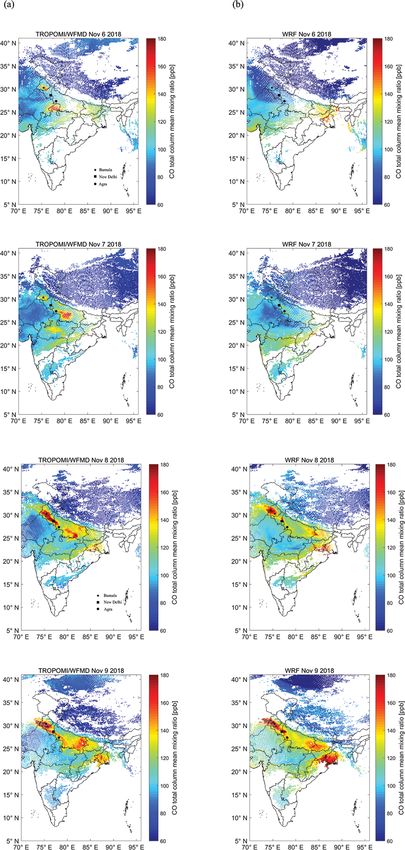
A. Vellalassery et al.: Understanding India’s air pollution with TROPOMI and WRF                                             5395

2018; Schneising et al., 2019, 2020a). TROPOMI measures            2     Data
with a high spatial (7 km × 7 km) and temporal resolution
(global daily coverage, not accounting for cloud and aerosol       2.1     TROPOMI column observations
contamination). The unprecedented data density, with a high
spatial and temporal resolution, makes TROPOMI useful for          The TROPOMI onboard the Sentinel-5 Precursor satellite
obtaining information from the city scale to regional scale.       (S5P), has been measuring various trace gases, including
The validation of the TROPOMI retrieval with ground-level          CO, since November 2017 (Landgraf et al., 2016; Borsdorff,
measurements and model simulations has confirmed the high          2018; Borsdorff et al., 2018; Schneising et al., 2019, 2020a).
quality of the measurements, with a high signal-to-noise ra-       The TROPOMI instrument consists of a shortwave infrared
tio, indicating the usefulness of the data collected (Borsdorff,   (SWIR), nadir-viewing imaging spectrometer, which mea-
2018; Borsdorff et al., 2018; Schneising et al., 2019, 2020a).     sures radiances around 2.3 µm wavelength, from which the
   In this study, we make use of CO observations from              total column mixing ratio (XCO) is retrieved (Schneising et
TROPOMI (see Sect. 2.1) and the surface measurement net-           al., 2019; Landgraf et al., 2016). Due to the wide swath of
work to investigate different regional sources of CO in terms      about 2600 km, the instrument is able to cover the whole
of their contribution to the total column and surface-level        globe on a daily basis, capturing full scenes of continuous ob-
concentrations during high pollution episodes in the win-          servations in cloud-free conditions (Schneising et al., 2019,
ter season. By comparing CO measurements with high-                2020a). As a result of the observation of reflected solar ra-
resolution model simulations generated by WRF–Chem-                diation in the SWIR part of the solar spectrum, TROPOMI
GHG, we aim to understand the contribution of different            yields atmospheric carbon monoxide measurements with
sources to the observed CO enhancement. In particular, we          high sensitivity to all altitude levels, including the planetary
focus on CO enhancement caused by the emissions from both          boundary layer, and is thus well suited for studying emissions
biomass burning and anthropogenic activities and their rela-       from fires (Schneising et al., 2020a).
tive roles in the severe air pollution of major cities nearby.        For this study, we use TROPOMI CO data for
This paper aims to address the following questions: (1) how        November 2018, retrieved using the scientific algorithm
large is the CO enhancement over northern India detected by        TROPOMI/WFM-DOAS, optimized to retrieve vertical
TROPOMI during the agricultural stubble burning period?            columns of carbon monoxide and methane simultaneously
(2) What is the regional contribution of CO emissions over         (Schneising et al., 2019). Additionally, we use TROPOMI
India during the entire year of 2018? (3) How good is the          operational CO data (TROPOMI/SICOR CO; Borsdorff,
agreement between the WRF–Chem-GHG and the observa-                2018; Borsdorff et al., 2018) to examine the consis-
tions, both at ground level and integrated across the column?      tency of these two observational products over India. The
(4) How does the column respond to the spatio-temporal vari-       TROPOMI/SICOR and TROPOMI/WFM-DOAS algorithms
ations in surface emissions, particularly biomass emissions?       differ in many aspects, including radiative transfer models,
(5) What is the role of different emission sources in terms of     inversion schemes and the quality filtering method used.
their contribution to the enhanced concentration level during      Whereas TROPOMI/WFM-DOAS retrievals are limited to
the high pollution episodes over India? An analysis focusing       cloud-free scenes, TROPOMI/SICOR aims to retrieve CO
on identifying the sources contributing to the high pollution      columns for cloudy ground pixels too. A global comparison
event in northern India during November 2017, using WRF            between these two data sets from December 2018 (Schneis-
modelling and TROPOMI preliminary operational data was             ing et al., 2019) shows a very similar spatial CO pattern for
reported in Dekker et al. (2019). Here, we present the anal-       both algorithms, with a high correlation coefficient of 0.98
ysis for the succeeding year, i.e. November 2018. Addition-        and a regression factor close to the 1 : 1 line, confirming a
ally, this study differs from the previous study as follows.       good agreement between the two data sets. An overview of
The present study (1) uses the retrievals from both algorithms     the TROPOMI data sets used in this study is provided in Ta-
of the Weighting Function Modified Differential Optical Ab-        ble 1, and additional details are provided in the following two
sorption Spectroscopy (TROPOMI/WFM-DOAS; Schneis-                  sub-sections.
ing et al., 2019; see Sect. 2.1) and TROPOMI Shortwave
Infrared Carbon Monoxide Retrieval (TROPOMI/SICOR;                 2.1.1    Scientific TROPOMI/WFMD CO product
Landgraf et al., 2016); (2) examines the regional distribution
of CO for the entire year, (3) employs different model config-     The WFM-DOAS retrieval algorithm was initially devel-
uration such as the model domain size, vertical eta levels, and    oped for the SCanning Imaging Absorption spectroMeter
planetary boundary layer scheme; (4) prescribes a different        for Atmospheric CartograpHY (SCIAMACHY) instrument
anthropogenic emission inventory that also includes hourly         on board the ENVISAT satellite (Buchwitz et al., 2006,
variations; and (5) utilizes the entire month, which includes      2007; Schneising et al., 2011, 2014) and has recently been
biomass burning and non-biomass burning periods to obtain          adjusted for XCO retrieval from TROPOMI (Schneising
a more detailed view of the dispersion to nearby places.           et al., 2019, 2020a). TROPOMI/WFM-DOAS uses a least
                                                                   squares approach, which retrieves XCO from the shortwave

https://doi.org/10.5194/acp-21-5393-2021                                            Atmos. Chem. Phys., 21, 5393–5414, 2021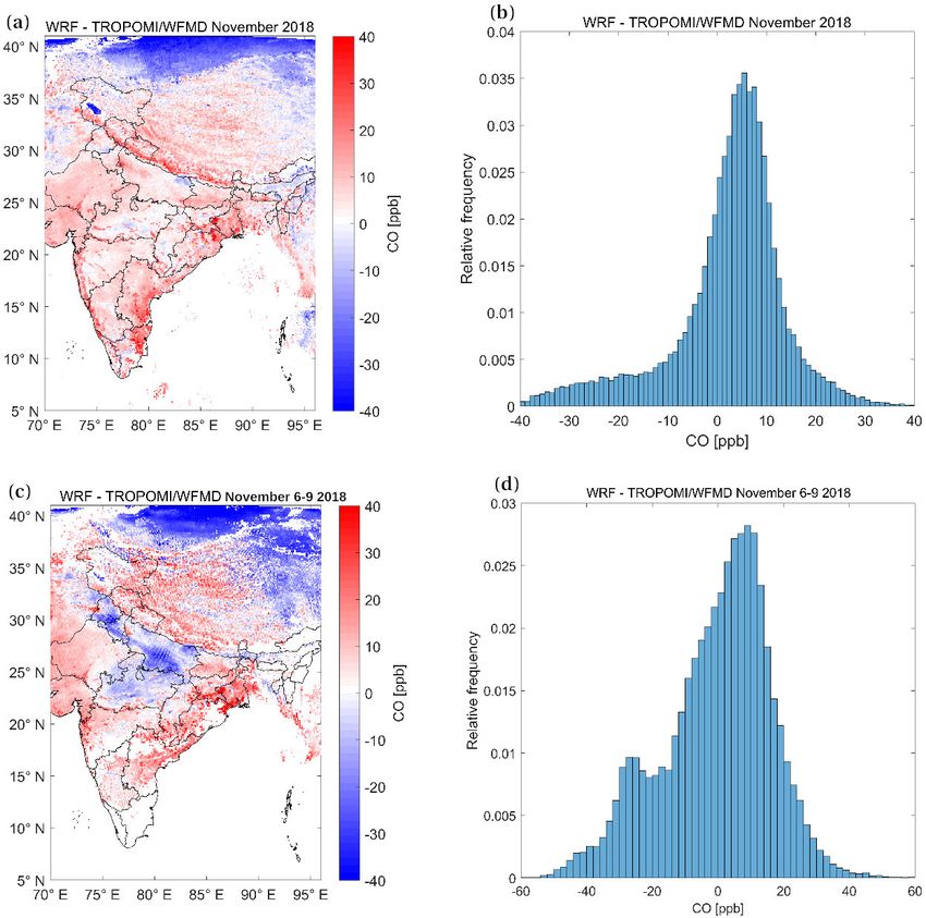
5396                                 A. Vellalassery et al.: Understanding India’s air pollution with TROPOMI and WRF

Table 1. Overview of the TROPOMI CO products used in this study.

            Data ID         Satellite data    Retrieval algorithm         Data access              Reference
            TROPOMI/        TROPOMI/          Weighting Function          (http://www.iup.         Schneising et al. (2019,
            WFMD            WFMD CO           Modified Differential       uni-bremen.de/carbon_    2020a)
                                              Optical Absorption          ghg/products/tropomi_
                                              Spectroscopy (WFM-          wfmd/, last access:
                                              DOAS)                       7 February 2020)
            TROPOMI/        TROPOMI/          Shortwave Infrared          (https://scihub.         Landgraf et al. (2016);
            SICOR           SICOR CO          Carbon Monoxide             copernicus.eu/, last     Borsdorff (2018); Bors-
                                              Retrieval (SICOR)           access: 24 August        dorff et al. (2018)
                                                                          2020)

infrared spectra recorded by the TROPOMI instrument. The              we have analysed CO measurements available from all sta-
TROPOMI/WFM-DOAS CO retrievals (hereafter referred                    tions for the period of 3–20 November 2018, measurement
to as TROPOMI/WFMD) have undergone direct validation                  stations that are too close to local emissions sources or show
with independent reference data from the worldwide total              extremely large and ambiguous variations in which the sta-
carbon column observing network (TCCON; Wunch et al.,                 bility of the analyser could be questioned were excluded for
2011), which consists of ground-based Fourier transform               the evaluation. All the stations used for this evaluation are
spectrometer (FTS) instruments with a well-controlled light           listed in Table 2.
path. TCCON measurements are calibrated to the World Me-
teorological Organization (WMO) scale. As per this vali-
dation, TROPOMI/WFMD XCO has a systematic error of                    3   WRF–Chem-GHG model
1.9 ppb (parts per billion) and a random error of 5.1 ppb
                                                                      We utilize a high-resolution modelling framework based on
(Schneising et al., 2019).
                                                                      a WRF–Chem-GHG (version 3.9.1.1; hereafter referred to
2.1.2    Operational TROPOMI/SICOR CO product                         as WRF) to simulate CO concentrations at a spatial reso-
                                                                      lution of 10 km × 10 km) and a temporal resolution of 1 h.
The Shortwave Infrared Carbon Monoxide Retrieval                      The model solves the compressible Euler non-hydrostatic
(SICOR) algorithm is used to retrieve the operational CO              equations and uses a terrain-following hydrostatic pressure
product (hereafter referred to as TROPOMI/SICOR; Land-                coordinate system in the vertical direction (Skamarock et
graf et al., 2016; Borsdorff, 2018; Borsdorff et al., 2018).          al., 2008). In our case, simulations have 39 vertical levels
The validation study of TROPOMI/SICOR with the CAMS                   extending from the surface to 50 hPa (∼ 20 km), and the
data shows a good agreement with global mean difference of            model domain describes a region with a spatial extent of
+3.2 % and a Pearson correlation coefficient of 0.97 (Bors-           3500 km × 2500 km, covering the Indian domain and some
dorff et al., 2018). For the Indian region, a 2.9 % difference        parts of Bangladesh, China, Nepal, and Pakistan.
was found with CAMS, with a standard deviation of 6 % and                For meteorological initial and boundary conditions, we
a Pearson correlation coefficient of 0.9 (Borsdorff, 2018). As        have taken fifth generation ECMWF reanalysis (ERA5)
per the validation of TROPOMI/SICOR with ground-based                 data, on an hourly basis, with a horizontal resolution of
total column measurements of TCCON, a mean bias of 6 ppb              0.25◦ × 0.25◦ . The model is re-initialized each day with
with a standard deviation of 3.9 and 2.4 ppb has been found           ERA5 meteorology and allowed a 6 h spin-up time. For CO
for clear and cloudy skies, respectively (Borsdorff, 2018).           concentration fields, initial and boundary conditions are pre-
                                                                      scribed from the Copernicus Atmosphere Monitoring Ser-
2.2     Ground-level observations                                     vice (CAMS re-analysis data). CAMS provides the esti-
                                                                      mated mixing ratios of CO, with a spatial resolution of
To assess the model performance against the surface-level             0.25◦ × 0.25◦ at a temporal resolution of 6 h on 60 verti-
measurements, we use measurements from ground-based                   cal levels. For CO simulations, we have mainly used anthro-
air quality monitoring network maintained by the Cen-                 pogenic and biomass burning emissions tracers from external
tral Pollution Control Board (CPCB) of India. The mea-                data sets. To represent anthropogenic contributions, we use
surements of CO are performed using CO analysers based                the global EDGAR emission inventory (Emission Database
on non-dispersive infrared spectroscopy, and the data are             for Global Atmospheric Research; version 4.3.2; the year
provided as 6 h averages via a publicly accessible online             2012) data at a spatial resolution of 0.1◦ × 0.1◦ . EDGAR
portal (https://app.cpcbccr.com/ccr/#/caaqm-dashboard-all/            provides global inventories for GHG emissions and air pol-
caaqm-landing/data, last access: 16 March 2020). Though               lutants on an annual basis, but we apply time factors in order

Atmos. Chem. Phys., 21, 5393–5414, 2021                                                 https://doi.org/10.5194/acp-21-5393-2021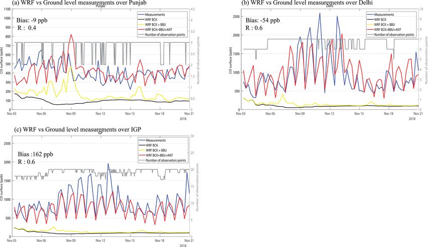
A. Vellalassery et al.: Understanding India’s air pollution with TROPOMI and WRF                                                    5397

Table 2. List of ground-level measurement stations used for this study.

     No.    Station name                                                             State           Latitude (◦ N)   Longitude (◦ E)
     1      Hardev Nagar, Bathinda                                                   Punjab                  30.23             74.90
     2      Civil Line, Jalandhar                                                    Punjab                  31.32             75.57
     3      Ratanpura, Rupnagar – Ambuja Cements                                     Punjab                  30.00             76.60
     4      National Institute of Solar Energy Gwal Pahari, Gurugram                 Punjab                  28.42             77.14
     5      Burari Crossing, Delhi                                                   Delhi                   28.72             77.20
     6      Delhi                                                                    Delhi                   28.55             77.25
     7      IGI Airport (Terminal 3), Delhi                                          Delhi                   28.56             77.11
     8      ITO, Delhi                                                               Delhi                   28.62             77.24
     9      Lodhi Road, New Delhi                                                    Delhi                   28.59             77.22
     10     Netaji Subhas University of Technology, Dwarka, Delhi                    Delhi                   28.60             77.03
     11     Patparganj, East Delhi                                                   Delhi                   28.62             77.28
     12     Sector 125, Noida                                                        Utter Pradesh           28.50             77.30
     13     Sanjay Palace, Agra                                                      Utter Pradesh           27.20             78.00
     14     Central School, Lucknow                                                  Utter Pradesh           26.88             80.93
     15     Ardhali Bazar, Varanasi                                                  Utter Pradesh           25.40             82.90
     16     Indira Gandhi Science Complex (IGSC) Planetarium Complex, Patna          Bihar                   25.60             85.10
     17     Ghusuri, Howrah                                                          West Bengal             22.61             88.34
     18     Padmapukur, Howrah                                                       West Bengal             22.56             88.27
     19     Rabindra Bharati University, Kolkata                                     West Bengal             22.62             88.38
     20     Victoria Memorial, Kolkata                                               West Bengal             22.54             88.34

to create hourly emissions. The time factors are based on the             main. The total CO is then calculated as CO total equals CO
step function time profiles, based on the TROTREP/POET                    background (BCK) plus CO anthropogenic (ANT) plus CO
profiles provided in Olivier et al., 2003. We use the CO                  biomass (BBU).
emission data from the Global Fire Assimilation System                       Utilizing the emission tracers mentioned above and
(GFAS) for the year of 2018 to represent biomass burning                  the multiple physics and chemistry options and dynamics
emissions. GFAS is a satellite-based fire emission inventory              schemes (see Table 3), model simulations of CO are per-
(http://apps.ecmwf.int/datasets/data/cams-gfas/, last access:             formed for the period 1–30 November 2018. To assess the
10 March 2019), which provides biomass burning emissions                  impact of small fires on our atmospheric CO mixing ratio
daily at a global horizontal resolution of 0.1◦ × 0.1◦ . The              simulations, we use another satellite-based fire inventory, the
inventory calculates the fire emissions by assimilating FRP               Global Fire Emissions Database version 4s (GFED4s), which
observations from MODIS instruments on the polar-orbiting                 includes small fires (Randerson et al., 2012; van der Werf et
satellites, Aqua and Terra, which observe the thermal radia-              al., 2017). The dry matter (DM) emissions from GFED4s are
tion from fire activities at wavelengths around 3.9 and 11 µm             converted to CO emissions, using emissions factors given in
(Kaiser et al., 2012). It achieves higher spatial and tempo-              Akagi et al. (2011).
ral (daily) resolution than almost any other inventory and can               The model setup does not include the deposition and
estimate near-real-time emissions. A number of studies have               chemical formation of CO from volatile organic compounds
reported the underestimation of GFAS in fire emissions due                (VOCs). Compared to the direct CO sources, such as an-
to the limitations of the MODIS instruments, which do not                 thropogenic and biomass burning emissions over the model
capture all active fires such as small fires (Cusworth et al.,            domain, the indirect source from VOC oxidation is much
2018; Dekker et al., 2019; Huijnen et al., 2016; Kaiser et al.,           smaller, and the deposition processes are minor compared
2012; Mota and Wooster, 2018; Pan et al., 2020).                          to the transport of CO out of the model domain (Dekker
   All these emissions fluxes are gridded to WRF’s Lam-                   et al., 2017). Also, the oxidation with the hydroxyl (OH)
bert conformal conic projection grid, with 10 km horizon-                 radical is not considered. Based on a few sensitivity simu-
tal resolution, conserving the total mass of emissions. These             lations, Dekker et al. (2017) reported a slight (4 %) net de-
fluxes are added to the first model layer and transported sep-            crease in enhancement when including chemical reactions of
arately as tagged tracers (Pillai et al., 2016). In order to ac-          CO and concluded that the CO enhancement pattern is hardly
count for the CO transported from the boundaries, we used                 affected by VOCs and OH oxidation.
CAMS CO data derived at the boundary conditions and refer
to this CO tracer as background, meaning the concentration
without considering any sources or sinks in the targeted do-

https://doi.org/10.5194/acp-21-5393-2021                                                     Atmos. Chem. Phys., 21, 5393–5414, 2021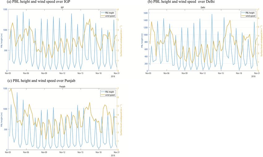
5398                                 A. Vellalassery et al.: Understanding India’s air pollution with TROPOMI and WRF

Table 3. Overview of WRF–Chem model set-up.

                 Domain                    Configuration                    Single domain with horizontal reso-
                                                                            lution of 10 km, with 307 × 407 grid
                                                                            points and 39 vertical levels.
                                           Vertical coordinates             Terrain-following hydrostatic pressure
                                                                            vertical coordinates
                                           Basic equations                  Non-hydrostatic
                                           Time integration                 Third order Runge–Kutta split explicit
                                           Time step                        60 s
                                           Spatial integration              A third and fifth order differentiation
                                                                            for vertical and horizontal advection,
                                                                            respectively.
                 Physics/dynamics          Radiation                        Rapid radiative transfer model
                 Schemes                                                    (RRTM) for long wave and Dudhia for
                                                                            short wave.
                                           Microphysics                     WSM 3 – classic simple ice scheme
                                           Planetary boundary layer (PBL)   YSU
                                           Surface layer                    Monin–Obukhov
                                           Land surface                     NOAH LSM
                                           Cumulus                          Grell–Devenyi ensemble scheme
                 Chemistry options         Chemical mechanism               Greenhouse gas tracer option (passive
                                                                            tracer) using previous simulations to
                                                                            initialize tracer fields.
                                           Emission input and               Setting (=16) for fluxes and emissions
                                           specification                    to passive tracers.

4     Methods                                                       kernel, cavgk , is calculated as follows:

                                                                                   1 Xn                  l     l

4.1    Comparison of WRF simulations with satellite                 cavgk = c +           ml (1 − Al ) (x T − x     .              (1)
                                                                                   m0 l=1
       column observations
                                                                       In this equation, l is the index of the vertical layer, n is the
To evaluate the performance of WRF, we have performed               number of vertical layers, and Al the corresponding column-
a comparison study on a daily and monthly basis using               averaging kernel of the TROPOMI/WFMD algorithm. c is
TROPOMI/WFMD column CO (XCO) data during the pe-                    the pressure-weighted column averaged dry air mole frac-
riod 1–30 November 2018 over the Indian domain. The                 tion calculated from model simulations. x T is the a priori dry
TROPOMI/WFMD data set also provides the column aver-                air mole fraction profile used by the TROPOMI/WFMD re-
aging kernel vector (AK) describing the vertical sensitivity        trieval algorithm, which is also provided in the data product,
of the retrieved CO column to the partial column at different       and x is the model simulation. ml is the mass of dry air for
vertical levels (Schneising et al., 2019). In order to compare      the corresponding layer, and m0 is the total mass of dry air.
the satellite data with model simulations quantitatively, we        For the comparison, we used only WRF simulations that cor-
have to use the AK to take into account the vertical sensitiv-      respond to the satellite sampling time. For a fair comparison
ity of the instrument. In the data set, the elements of the AK      between the satellite observations and model simulations, the
mostly have values close to 1, meaning that the instrument          averaging kernel matrix and a priori profile for each retrieval
is sensitive to the full column of CO. As such, the prior esti-     have been applied to the corresponding model output as ex-
mates have a negligible contribution to the retrieved columns.      plained in Eq. (1). For the ease of the statistical analysis,
To compare the simulated concentration fields with the satel-       the observations, though comparable to the model resolution,
lite observations, the simulated pressure-weighted column-          are gridded to the WRF spatial resolution of 10 km × 10 km.
averaged dry air mole fraction after applying the averaging         Both TROPOMI/WFMD and WRF averaged data for the

Atmos. Chem. Phys., 21, 5393–5414, 2021                                                https://doi.org/10.5194/acp-21-5393-2021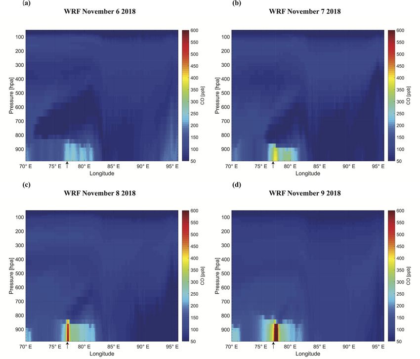
A. Vellalassery et al.: Understanding India’s air pollution with TROPOMI and WRF                                                   5399

month of November and the period of 6–9 November (en-
hanced biomass burning period as per the GFAS data) are
utilized in this study to investigate the column enhancement
by fire CO and their distribution over the study domain. Dur-
ing the enhanced biomass burning period, a definite enhance-
ment in XCO is found over the biomass burning hotspot. The
monthly averaged map shows decreased concentration levels
over these hotspots, which is attributed to the CO concentra-
tion dispersion resulted by changing weather conditions.

4.2    Comparison of WRF simulations with ground-level
       observations

To evaluate the model performance at the surface level, we
have performed a comparison study with the CO in situ mea-
surements obtained from the ground-level pollution measure-
ment stations. We use the data collected from 20 measure-
ment stations within the IGP region, and evaluation is done
against each station data. In order to see overall agreement
for different regions in the IGP, we have averaged the data
                                                                   Figure 1. India is partitioned into the following five different areas
temporally using only the stations within the corresponding
                                                                   for analysis: northeastern India (NEI), central India (CI), southern
regions (Delhi, Punjab, and the IGP). The entire month is not      India (SI), the Indo-Gangetic Plain (IGP), and northern India (NI).
used here due to the existence of data gaps from several sta-
tions. In order to avoid very localized influence and noise in
the observed data, the 1 h data sets are temporally averaged       This is also consistent with the distribution of total fire counts
to 6 h resolution.                                                 over IGP region during the post-monsoon period, as seen in
                                                                   Kulkarni et al. (2020). Over the IGP, the fire CO emissions
5     Results and Discussions                                      show evident monthly variations, with a higher emission dur-
                                                                   ing the post-monsoon time compared to the pre-monsoon pe-
5.1    Regional and seasonal variation of fire CO emission         riod. About 73 % of the country’s total fire CO emissions
                                                                   during the post-monsoon period are from the IGP region.
In order to examine the spatio-temporal variations of the          Of these IGP post-monsoon emissions, 70 % come from the
monthly fire CO emission, we have divided the entire region        northwestern states of the IGP (Punjab and Haryana). Over
into five sub-regions, as shown in Fig. 1. The fire CO emis-       this region, 25 % of the total fire CO emissions happened
sions show significant spatial and temporal variations, with       within a short period during 6–9 November, which accounts
predominant emissions over the Indo-Gangetic Plain (IGP),          for about 18 % of the country’s post-monsoon total fire CO
central India (CI), and northeastern India (NEI).                  emissions. During the monsoon time, all regions are found
   Figure 2 illustrates the integrated monthly fire CO emis-       to have fewer fire emissions, which can be attributed to the
sion for those regions in 2018. In most parts of India, the fire   fact that rainfall leads to suppressed fire activity. In addition
CO emissions peak during the March–April (pre-monsoon)             to the minimal possibility of fire activities during the rainy
period, accounting for about 76 % of the annual emissions.         season, note that MODIS has only a limited capability to
This is consistent with a study based on the fire counts anal-     detect fire emissions over a cloudy scene. It should also be
ysis from 1998–2009, which reported that more than 75 %            noted that very small fires involved can be missed due to
of the annual fires occurred during March–April (Sahu et           MODIS instruments limitations, which may underestimate
al., 2015). Fire CO emissions during March are significantly       the fire CO emissions. With a finer spatial resolution of VI-
higher when compared to other months, accounting for about         IRS (375 m) than MODIS (1 km), VIIRS detected ∼ 20 %
55 % of the annual emissions for India. Although having a          more active fires at the spatial scale of 0.02◦ × 0.02◦ over
small geographical area, the fire activities over northeastern     Punjab and Haryana during the post-monsoon season (Liu et
India (NEI) made a significant contribution (57 %) to emis-        al., 2019).
sions during pre-monsoon months, while the IGP contributed            The observed monthly variations in fire emissions are
only about 5 %. Central (CI) and southern regions (SI) of In-      mainly due to factors such as post-harvest crop residue burn-
dia add about 33 % towards the pre-monsoon fire CO emis-           ing, meteorological conditions (dry weather), and land-use
sions, while northern India (NI) shows fewer emissions dur-        practices (Habib et al., 2006). The fire activities during post-
ing the whole year. However, emission spikes are seen in the       and pre-monsoon periods in India are mostly associated with
IGP during the October–November (post-monsoon) period.             the high level of crop residue burning during the post-harvest

https://doi.org/10.5194/acp-21-5393-2021                                             Atmos. Chem. Phys., 21, 5393–5414, 2021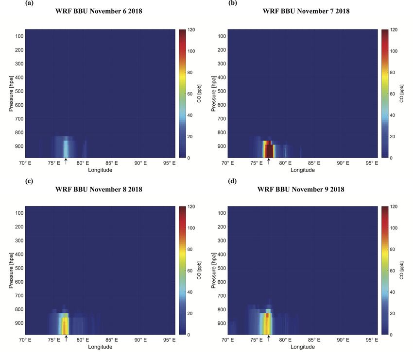
5400                                  A. Vellalassery et al.: Understanding India’s air pollution with TROPOMI and WRF

Figure 2. (a) The monthly integrated GFAS fire CO emissions (mg/m2 per month) over different regions of India (as seen in Fig. 1) during
the year of 2018. (b) Integrated GFAS fire CO emission during 6–9 November 2018.

seasons (Sahu et al., 2015). Crop residue burning after har-          ing that occurred over the Punjab region. The consistency
vesting is a general practice used by farmers to clear the land       check between two retrieval products (TROPOMI/WFMD
for the next crop. Over the IGP, there are mainly two sea-            and TROPOMI/SICOR) has resulted in a very similar spa-
sonal crop seasons, known as kharif (primarily rice) and rabi         tial CO pattern for both algorithms, with a high correlation
(mainly wheat), which are harvested during post- and pre-             coefficient of 0.97, confirming the robustness of our find-
monsoon seasons, respectively (Sahu et al., 2015). This re-           ings between the two data sets over India (see Table 4).
sults in temporal variations in residue burning emissions over        During early winter (November and December), the shal-
the IGP. Compared to other parts of the IGP, the northwest-           low planetary boundary layer (PBL) and low wind speed
ern part of the IGP has the greatest preponderance of crop            cause locally emitted gases to be trapped in the lower at-
residues during the post-monsoon season (Singh and Pani-              mosphere, which is considered to be the primary cause for
grahy, 2011). Consistent with the spatial and seasonal dif-           high concentrations during this period. For a better under-
ferences in agricultural practices, we see a high level of fire       standing of the role of transport and CO emissions from
CO emissions in this region during the short period of 6–9            biomass burning to the distribution over the domain, we uti-
November.                                                             lized WRF model simulations and performed a comparison
                                                                      study with the TROPOMI/WFMD observations, as explained
5.2    Enhanced XCO as observed by the satellite                      in Sect. 4.1.

Figure 3a shows the column CO dry mixing ratio retrieved              5.3     Validation of WRF
from TROPOMI/WFMD over the Indian domain, averaged
for the entire month of November and 6–9 November (most               5.3.1    Agreement with column observations
intense biomass burning period). During this period, higher
values of column CO are observed over the northern part of            We compared WRF simulations with TROPOMI/WFMD ob-
India, particularly over the IGP region, compared to the other        servations averaged over the days of peak burning and over
regions of India, showing higher values during the biomass            the full month of November 2018. Figure 3 shows these com-
burning period than the monthly average. A distinct enhance-          parisons. Both the satellite and the model show a higher level
ment in XCO can be observed during the biomass burning                of column CO over the IGP region than over any other re-
period, specifically over the states of Punjab and Haryana,           gion of the domain. In the monthly averaged plots, the model
with a distribution plume towards the southeasterly direc-            slightly overestimates (by about 10 ppb) the XCO in most
tion, including the regions of Delhi and Agra. Note that this         parts of the domain. Between the monthly averaged observa-
emission hotspot is also seen in the GFAS inventory during            tions and the simulations, we find a mean difference of 7 ppb,
the biomass burning period (Fig. 2). Consistency between the          with a standard deviation of 8 ppb and a correlation coeffi-
GFAS inventory and satellite observations suggests that the           cient of 0.87 (Fig. 4). Given that both CO and particulate
XCO enhancement over the northwestern part of the IGP dur-            matter (PM) are usually co-emitted, and there exists a rea-
ing 6–9 November can be attributed to the crop residue burn-          sonably high correlation between them during high pollution

Atmos. Chem. Phys., 21, 5393–5414, 2021                                                  https://doi.org/10.5194/acp-21-5393-2021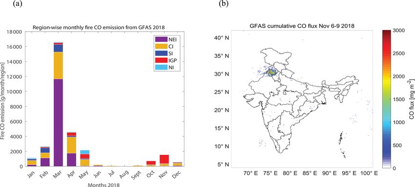
A. Vellalassery et al.: Understanding India’s air pollution with TROPOMI and WRF                                                  5401

Table 4. Comparison between TROPOMI/WFMD and TROPOMI/SICOR products over India during the burning period and the full month
of November 2018. Abbreviations N, MB, SD, and R correspond to the number of observations, mean bias, standard deviation of differences,
and correlation coefficient, respectively.

                       Peak burning period only          N (TROPOMI/SICOR) – 93 416
                       (6–9 November 2018)               N (TROPOMI/WFMD) – 98 093
                                                         MB (TROPOMI/SICOR–TROPOMI/WFMD) –
                                                         1.85 ppb
                                                         SD (TROPOMI/SICOR–TROPOMI/WFMD) – 4.86 ppb
                                                         R (TROPOMI/SICOR vs. TROPOMI/WFMD) – 0.97
                       All of November 2018              N (TROPOMI/SICOR) – 555 724
                                                         N (TROPOMI/WFMD) – 638 215
                                                         MB (TROPOMI/SICOR–TROPOMI/WFMD) –
                                                         1.72 ppb
                                                         SD (TROPOMI/SICOR–TROPOMI/WFMD) – 4.27 ppb
                                                         R (TROPOMI/SICOR vs. TROPOMI/WFMD) – 0.97

Figure 3. CO total column mixing ratios averaged for (a) TROPOMI/WFMD and (b) WRF over all of November 2018 (left panel) and from
6–9 November 2018 (right panel).

episodes, the reported enhanced CO can also be a good indi-           rate prediction of particulate matter needs aerosol–chemistry
cator of increased PM10 and PM2.5 that are associated with            modelling, since PM concentration is affected by heteroge-
bad air quality and health impacts. As a first-order approx-          neous chemistry and wet and/or dry removal processes, un-
imation, a high episodic PM estimation can be made using              like CO which is mainly affected by atmospheric transport
PM and/or CO linear conversion factors. However, the accu-            and mixing at regional scales.

https://doi.org/10.5194/acp-21-5393-2021                                                Atmos. Chem. Phys., 21, 5393–5414, 2021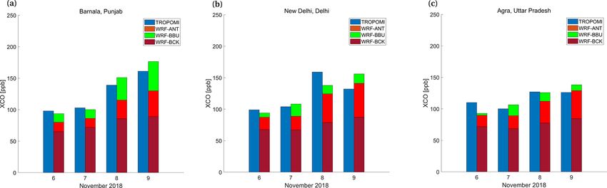
5402                                   A. Vellalassery et al.: Understanding India’s air pollution with TROPOMI and WRF

Figure 4. (a) Differences in CO total column mixing ratios (WRF – TROPOMI/WFMD) averaged over the month of November 2018. (b)
Histogram of the differences. (c) Same as panel (a) but restricting the period to 6–9 November 2018. (d) Same as panel (b) but restricting
the period to 6–9 November 2018.

   During the biomass burning period, the model underes-               with a peak on 9 November with a value of approximately
timates (by about 10–15 ppb) the enhancement over Punjab               165 ppb. Both observations and simulations suggest a south-
and some central parts of Uttar Pradesh, while overestimating          easterly transport of this plume, which increases the CO con-
(by about 15–20 ppb) enhancements over the eastern parts of            centration over Delhi and Agra during 8 and 9 November.
IGP, including West Bengal and some parts of Bihar. Daily              Over Delhi, the TROPOMI/WFMD XCO reached a max-
retrievals of TROPOMI/WFMD and the corresponding sim-                  imum on 8 November, while modelled CO showed a de-
ulations for the biomass burning period are shown in Fig. 5.           lay with a maximum concentration on 9 November. On 9
An enhanced XCO is reported in both observations and sim-              November, the observation shows more dispersed XCO over
ulations over the state of Punjab, starting from 6 Novem-              Delhi towards the southeasterly direction in comparison with
ber and gradually increasing in the following days. During             model simulations. Over Agra, which is located far away
this period, the plume is seen to be partly transported in a           from the pollution hotspot but along the transport pathway,
southeasterly direction along the regions of Delhi and Agra.           an increase in XCO, which is consistent with that over the
Over the IGP there exists an overall slight underestimation by         other two cities, is found.
WRF in comparison to TROPOMI during this period, with a                   Based on VIIRS AOD (aerosol optical depth) and WRF–
mean model-to-observation difference of −2.7 ppb.                      Chem simulations using different chemical and meteorology
   Figure 6 shows the temporal evolution of the CO concen-             boundary conditions and biomass burning emissions, Rooz-
tration in three cities (Barnala, New Delhi, and Agra) located         italab et al. (2021) assessed the model performance over the
along the transport pathway of pollution. The data are aver-           IGP region during an intensive fire period in November 2017
aged in a 100 km × 100 km square around the centre of each             and reported an underestimation of AODs for the entire IGP
city. During the biomass burning period, the XCO over Bar-             region, except for Punjab. Furthermore, Kumar et al. (2020)
nala (Punjab) shows a steady positive increment with time,             found a considerable impact of uncertainties in the WRF me-

Atmos. Chem. Phys., 21, 5393–5414, 2021                                                   https://doi.org/10.5194/acp-21-5393-2021
A. Vellalassery et al.: Understanding India’s air pollution with TROPOMI and WRF                                       5403

Figure 5. (a) Daily column CO observations from TROPOMI/WFMD and (b) the co-located WRF simulation for 6–9 November 2018.

https://doi.org/10.5194/acp-21-5393-2021                                         Atmos. Chem. Phys., 21, 5393–5414, 2021
5404                                 A. Vellalassery et al.: Understanding India’s air pollution with TROPOMI and WRF

Figure 6. Carbon monoxide (CO) total column mixing ratios over (a) Barnala, (b) New Delhi, and (c) Agra for individual days from 6–9
November 2018.

teorology on simulated PM2.5 concentrations over IGP dur-           54 ppb are found for Punjab and Delhi. For the IGP region,
ing the crop residue burning period in November 2017. Note          the model underestimates the observed enhancements con-
that our study also reports a slight underestimation of WRF         siderably, resulting in a mean bias of 162 ppb. The observed
compared to TROPOMI CO observations over IGP during                 underestimation of WRF can be attributed to the local source
the biomass burning period. Though we cannot directly com-          enhancements at the ground-level stations, which are located
pare AOD and/or PM2.5 results during November 2017 from             close to the cities. For the Punjab region, the model CO sur-
previous studies with our CO simulations during November            face concentration shows the influence of biomass burning,
2018, the results indicate shortcomings in the model that can       starting from 6 November with a maximum of 800 ppb on 8
be refined by better representation of atmospheric transport        November. Unlike the Punjab region, the concentration pat-
(including model initialization) and emission.                      terns over Delhi and the IGP show a steadily increasing trend
   The details in Table 4 confirm the minimal impact of the         from 6 to 13 November, with a subsequent reduction in mix-
differences in satellite retrieval algorithms on our results.       ing ratios for the remaining days. Among these study regions
This analysis suggests a promising usage of TROPOMI ob-             during this period, the lowest and highest surface CO levels
servations for understanding the details of hotspot emissions       are observed over the regions of Punjab (mean – 500 ppb)
and the distribution of transport. The model is able to capture     and Delhi (mean – 1500 ppb), respectively. Except for Pun-
many of these spatial and temporal patterns, supporting the         jab, we see better mean bias when excluding nighttime val-
potential use of WRF via inverse modelling to infer hotspot         ues (21 ppb for Delhi and 141 ppb for the IGP region), as
emissions using column measurements.                                the uncertainty from mixing height simulations is larger dur-
                                                                    ing nighttime compared to daytime. Surprisingly the overall
5.3.2   Agreement with ground-level observations                    underestimation increased in Punjab when using only day-
                                                                    time values, indicating a considerable underestimation of lo-
Figure 7 shows the model evaluation with ground-level mea-          cal emission sources, likely from the biomass emission in-
surements over the regions IGP, Delhi, and Punjab for a pe-         ventory. Note that the GFAS fire emissions may be under-
riod from 3 to 20 November 2018. The location of ground-            estimated (Mota and Wooster, 2018). The GFAS fire emis-
level measurement stations used for this study is shown in          sions are partly based on the MODIS satellite instrument,
Fig. 8. The entire month is not used here due to the ex-            and the limited resolution of the instrument misses many
istence of data gaps from several stations. Taking various          small fires, including biomass burning over India (Cusworth
ground-based stations over the IGP, Delhi, and Punjab, we           et al., 2018). A comparison of post-monsoon fire CO emis-
see an overall agreement between the model and measure-             sions over Punjab and Haryana, as estimated from five global
ments, with a correlation coefficient of 0.6 (for the IGP),         inventories for the period from 2003 to 2016, indicates the
0.6 (Delhi), and 0.41 (Punjab). Among these three study re-         limitation of satellite-derived fire products and the associ-
gions, a lower correlation is found for the Punjab region in        ated uncertainties in the CO fire emissions (Liu et al., 2019).
which measurement sites are very close to the biomass burn-         Overall, the results show that the model simulation, at a high
ing hotspots, therefore showing a larger variability associated     spatial resolution, is capable of capturing the CO enhance-
with biomass emissions compared to other stations. These            ment and reduction pattern at most of the stations; however,
variations are not fully reproduced by the model, resulting         there is a non-trivial mean bias which can be attributed to
in lower correlations over the Punjab region. Though the            issues with simulating transport (including the emission re-
model is able to follow the temporal variation in the surface-      lease height) and PBL dynamics in WRF as well as the vari-
level CO concentrations, overall underestimations of 9 and

Atmos. Chem. Phys., 21, 5393–5414, 2021                                               https://doi.org/10.5194/acp-21-5393-2021
A. Vellalassery et al.: Understanding India’s air pollution with TROPOMI and WRF 5405
ability in emission fluxes (both EDGAR and GFAS), which ber over Delhi, however, the average contribution from fire
is likely to not be sufficiently well represented in the emis- dropped to 4 % compared to 85 % in the case of the anthro-
sion inventories used. pogenic contribution.
To examine the impact of missed active fires on our WRF
5.4 Contribution of different sources to the observed results, we perturb GFAS fire emissions by a factor of 50 %
concentration and quantify how this perturbation affects the size of the
anomaly in CO mixing ratios over the IGP region. Note that
To further investigate the contribution of different emission VIIRS detected ∼ 20 % more active fires during the post-
sources to the observations, we use the tagged tracer op- monsoon season over Punjab and Haryana. Using the per-
tion in WRF and separate the contributions from different turbed GFAS emissions, we estimate that the relative in-
sources, as shown in Figs. 6 and 7. Note that the signals crease in modelled XCO contribution arises from increased
contributing to satellite observations are difficult to disen- biomass emissions. With the increased emissions, we see an
tangle without underlying assumptions or the availability of increment of XCO contribution, ranging approximately from
multi-tracers such as CO and nitrogen oxides and the follow- 5 to 25 ppb, during biomass burning period over IGP region,
ing: NOx and NO∗y (NO∗y includes NOx , peroxyacetyl nitrate mostly over Punjab, Haryana, and Delhi (see Figs. S3 and
(PAN), organic nitrates, nitric acid (HNO3 ), and dinitrogen S5). As for the model observation performance statistics, a
pentoxide (N2 O5 ; e.g. Wang et al., 2002). The relative con- slight improvement is found for XCO over IGP region with
tributions of different emission sources and processes to the this perturbed simulation (see Table S1).
WRF CO column, as summarized in Table 4, clearly indi- For allocating small fires over the model domain, we use
cate the dominance of anthropogenic signals over biomass the GFED4s fire product, including fire fractions stemmed
burning signals on the XCO enhancements (see Figs. S1 and from the small fire-burned area. The small fire boost in
S2 in the Supplement). The significant impact of background GFED4s is calculated based on active fire hotspots and
signal, owing to the advection from the domain boundary burned area observations from MODIS surface reflectance
throughout the column, indicates the influence of far-field (Randerson et al., 2012). The difference in fire emission
fluxes and large-scale transport patterns on column CO (see fields in GFED4s, relative to GFAS, is derived over the model
Fig. 6). During the biomass burning period, there exists a domain and is applied to WRF to quantify the fire CO contri-
considerable contribution of biomass burning emissions to bution that also includes small fires. While including small
the column mixing ratios, particularly over the Punjab region fires based on GFED4s has improved the model observa-
(14 %). Relatively low contributions of biomass burning sig- tion mean bias over IGP region for surface CO mixing ratio
nals to the column in Delhi and the IGP compared to Punjab during biomass burning period, we see a minimal improve-
indicates the dominant contribution of surface CO emission ment for XCO (see Table S1). Enhancing the fire emission
to the column in Punjab, which is where the biomass emis- by incorporating small fires resulted in an overall increment
sions originated. It also suggests the possibility of less dilu- of XCO concentration ranging from 20 to 40 ppb; however,
tion of surface emissions during wintertime, enhancing the most of the contributions arising from small fires are seen
total column mixing ratios. The effect of advected biomass only over Punjab and some parts of Haryana (see Figs. S3
burning signals in terms of their contribution to the column and S5). Based on GFED4s, we quantify the effect of small
can be seen over Delhi (12 %); however, this effect becomes fires on the modelled atmospheric CO plumes. The addition
smaller in the IGP (5 %) due to further dispersion. of small fires contributed to an increment of 12.2 % surface
The diurnal variation in the surface-level CO concentra- CO over Punjab and Haryana, and the small fire contribu-
tion pattern is due to the diurnal variation in the plane- tion is reduced to 8.6 % and 4.3 % over Delhi and IGP, re-
tary boundary layer height (PBLH) combined with strong spectively. In the case of XCO, there exists only a minimal
sources of CO at the surface. The contribution from emis- impact of small fires on mixing ratios, which are estimated
sions sources over the Delhi, IGP, and Punjab regions for to be 2.5 % over Punjab and Haryana, 1.4 % over IGP, and
the period of 3–20 and, specifically, 6–9 November are also 0.8 % over Delhi. The difference in the contribution of small
summarized in Table 5. For all regions, the influence of back- fires between surface CO and XCO can be explained by the
ground CO concentrations to the surface-level CO observed meteorology conditions that prevailed (see Sect. 5.5).
variability is minimal, as expected (see Fig. 7). The back- Overall, our findings suggest that the enhanced CO levels
ground influence is expected to be smaller for surface CO in during pollution episodes over Delhi and the greater part of
urban areas, where the CO fraction from local anthropogenic IGP are affected by biomass burning. However, a more sig-
emissions dominates the background signals. At ground level nificant contribution comes from anthropogenic emissions.
in Delhi and the IGP, a detectable enhancement in surface Unlike the surface CO mixing ratios, the majority of the
CO due to fire CO is found only during 6–9 November. Dur- column CO mixing ratio is contributed by the background
ing this period, the average contribution of biomass burning signal. A recent study conducted by Dekker et al. (2019)
to the ground-level concentration is 10 %, while the anthro- concluded that there exists an underestimation in GFAS fire
pogenic contribution is 79 %–83 %. During 3–20 Novem- emission data over the Indian region. This is also supported
https://doi.org/10.5194/acp-21-5393-2021 Atmos. Chem. Phys., 21, 5393–5414, 20215406 A. Vellalassery et al.: Understanding India’s air pollution with TROPOMI and WRF Figure 7. Ground-level CO measurements and WRF model simulations for the period 3–20 November 2018 over (a) the IGP region, (b) Delhi, and (c) Punjab. Note that different y-axis scale ranges are used in the panels for a better visualization of the signals. Figure 8. Map showing the locations of sites used for model evaluation. The yellow contour represents the IGP region. The inset shows the broader region for context. Atmos. Chem. Phys., 21, 5393–5414, 2021 https://doi.org/10.5194/acp-21-5393-2021
A. Vellalassery et al.: Understanding India’s air pollution with TROPOMI and WRF                                            5407

Table 5. Contributions from different emissions sources to the CO concentration between 6–9 and 3–20 November 2018. Abbreviations
ANT, BBU, and BCK represent anthropogenic, biomass burning, and background signals, respectively (see Sect. 3).

                 Period           CO                 Delhi                  Punjab                   IGP
                                             ANT     BBU     BCK     ANT     BBU     BCK    ANT     BBU     BCK
                 6–9 Nov 2018     Column     35 %    12 %    53 %    21 %    14 %    65 %   32 %     5%     63 %
                                  Surface    83 %    10 %     7%     49 %    38 %    13 %   79 %    10 %    11 %
                 3–20 Nov 2018    Column     43 %     6%     51 %    25 %     8%     67 %   34 %     3%     63 %
                                  Surface    86 %     4%     10 %    60 %    17 %    23 %   82 %     4%     14 %

by our study in which we find that the underestimation of           regions, a less negative correlation of CO with PBLH and
the total CO concentration in Punjab during biomass burn-           wind speed is observed for Punjab. It suggests that, when
ing period and a part of this model observation mismatch            compared to Delhi and the IGP, the surface-level CO varia-
can be attributed to the underestimation of modelled fire           tion over the Punjab region cannot be explained by meteorol-
CO contribution. Over the Punjab region, biomass burning            ogy alone. Here the local emission activities, such as biomass
played a significant role in determining the ground-level CO        burning, explain more of the variability in surface-level CO.
measurements, especially during 6–9 of November during              A gradual increase in surface CO levels was observed from
which enhanced fire activities occurred. This has contributed       3 to 13 November during which an overall decrease in PBL
considerably to the column mixing ratio that is detected by         height and surface-level wind speed took place. The highest
TROPOMI. On average, for 3–20 November, 17 % of the to-             CO values around Delhi were found during 11–13 Novem-
tal ground-level CO concentration over the Punjab region is         ber, just before the winds and PBL height were increasing.
on account of fire CO emission, whereas for 6–9 November               Figures 10 and 11 provide transport patterns involving
the share is about 38 %.                                            the vertical distribution of CO biomass burning contribution
                                                                    and total CO mixing ratio, respectively, during the biomass
5.5   Effect of meteorology                                         burning period. Vertical cross sections show an impact of
                                                                    fire emission over Delhi during the biomass burning period
Usually pollution episodes during winter are the result of me-      (40 to 120 ppb), peaking its boundary layer CO contribution
teorological conditions due to low wind speed and a shallow         (>110 ppb) on 7 November (Fig. 10). On the other hand,
boundary layer (PBL height). To further analyse the effect of       the total CO shows peak values (>550 ppb) on 9 Novem-
meteorological conditions, we use WRF-simulated meteorol-           ber, indicating a significant additive contribution from an-
ogy due to the lack of observations of wind and PBL height in       thropogenic fluxes, in addition to biomass burning, together
this region. An inter-model comparison of WRF meteorology           with the winter meteorology conditions that prevailed over
with corresponding variables from reanalysis data provided          the region (see Fig. 11). A consistently low PBL height can
by Modern-Era Retrospective Analysis for Research and Ap-           be clearly seen during these days, which traps CO plumes in
plications, version 2 (MERRA-2) is performed to assess the          the lower boundary layer due to less extent of vertical mix-
overall agreement (see Table S2 and Fig. S6). Note that             ing. These findings suggest that the meteorological condi-
MERRA-2 is an assimilation product at an approximate spa-           tions have a large impact on the surface-level CO concen-
tial resolution of 0.5◦ × 0.625◦ , publicly available online at     tration, especially over the IGP and Delhi. Our results are
https://gmao.gsfc.nasa.gov/reanalysis/MERRA-2/ (last ac-            consistent with Dekker et al. (2019), who identified that the
cess: 14 January 2021). More information on MERRA-2 and             meteorological conditions contributed significantly to the en-
the assimilation system can be seen in Gelaro et al. (2017).        hancement of CO mixing ratios at the ground level during
Figure 9 demonstrates the influence of the PBL height and           November 2017. Similarly, Kariyathan et al. (2020), by us-
surface-level wind speed to the observed CO level. We found         ing a-temporal emission fields and a Lagrangian modelling
a negative correlation of CO with modelled PBLH (−0.83              framework, found a considerable impact of meteorological
– IGP; −0.73 – Delhi; −0.56 – Punjab) and wind speed                conditions during November 2017 that contributed to the en-
(−0.40 – IGP; −0.62 – Delhi; −0.24 – Punjab) for Novem-             hancements of trace gases over Delhi. Together with strong
ber 2018. Similar correlations of CO with modelled PBLH             emissions (anthropogenic and biomass burning), they found
(−0.87 – IGP; −0.83 – Delhi; −0.65 – Punjab) and wind               that these enhancements could be several orders of magni-
speed (−0.46 – IGP; −0.70 – Delhi; −0.26 – Punjab) exist            tude higher compared to other seasons.
for the biomass burning time period of 6–9 November 2018.
A strong negative relation between PBL height and CO level
is seen, indicating the impact of meteorology on the diur-
nal variation of surface-level CO concentration. Among the

https://doi.org/10.5194/acp-21-5393-2021                                             Atmos. Chem. Phys., 21, 5393–5414, 2021
You can also read