Version 4 CALIPSO Imaging Infrared Radiometer ice and liquid water cloud microphysical properties - Part I: The retrieval algorithms - Recent
←
→
Page content transcription
If your browser does not render page correctly, please read the page content below
Atmos. Meas. Tech., 14, 3253–3276, 2021
https://doi.org/10.5194/amt-14-3253-2021
© Author(s) 2021. This work is distributed under
the Creative Commons Attribution 4.0 License.

Version 4 CALIPSO Imaging Infrared Radiometer ice and liquid
water cloud microphysical properties – Part I: The retrieval
algorithms
Anne Garnier1 , Jacques Pelon2 , Nicolas Pascal3 , Mark A. Vaughan4 , Philippe Dubuisson5 , Ping Yang6 , and
David L. Mitchell7
1 Science Systems and Applications, Inc., Hampton, VA 23666, USA
2 Laboratoire Atmosphères, Milieux, Observations Spatiales, Sorbonne University, Paris, 75252, France
3 AERIS/ICARE Data and Services Center, Villeneuve-d’Ascq, 59650, France
4 NASA Langley Research Center, Hampton, VA 23681, USA
5 Laboratoire d’Optique Atmosphérique, Université de Lille, Villeneuve-d’Ascq, 59655, France
6 Department of Atmospheric Sciences, Texas A&M University, College Station, TX 77843, USA
7 Desert Research Institute, Reno, NV 89512, USA

Correspondence: Anne Garnier (anne.emilie.garnier@nasa.gov)

Received: 25 September 2020 – Discussion started: 30 November 2020
Revised: 17 March 2021 – Accepted: 18 March 2021 – Published: 4 May 2021

Abstract. Following the release of the version 4 Cloud-            more, the clear-sky mask has been refined compared to V3
Aerosol Lidar with Orthogonal Polarization (CALIOP)                by taking advantage of additional information now available
data products from the Cloud-Aerosol Lidar and Infrared            in the V4 CALIOP 5 km layer products used as an input to the
Pathfinder Satellite Observations (CALIPSO) mission, a new         IIR algorithm. After sea surface emissivity adjustments, ob-
version (version 4; V4) of the CALIPSO Imaging Infrared            served and computed brightness temperatures differ by less
Radiometer (IIR) Level 2 data products has been developed.         than ±0.2 K at night for the three IIR channels centered at
The IIR Level 2 data products include cloud effective emis-        08.65, 10.6, and 12.05 µm, and inter-channel biases are re-
sivities and cloud microphysical properties such as effective      duced from several tens of Kelvin in V3 to less than 0.1 K
diameter and ice or liquid water path estimates. Dedicated         in V4. We have also improved retrievals in ice clouds hav-
retrievals for water clouds were added in V4, taking advan-        ing large emissivity by refining the determination of the ra-
tage of the high sensitivity of the IIR retrieval technique to     diative temperature needed for emissivity computation. The
small particle sizes. This paper (Part I) describes the im-        initial V3 estimate, namely the cloud centroid temperature
provements in the V4 algorithms compared to those used in          derived from CALIOP, is corrected using a parameterized
the version 3 (V3) release, while results will be presented in     function of temperature difference between cloud base and
a companion (Part II) paper. The IIR Level 2 algorithm has         top altitudes, cloud absorption optical depth, and CALIOP
been modified in the V4 data release to improve the accu-          multiple scattering correction factor. As shown in Part II, this
racy of the retrievals in clouds of very small (close to 0) and    improvement reduces the low biases at large optical depths
very large (close to 1) effective emissivities. To reduce biases   that were seen in V3 and increases the number of retrievals.
at very small emissivities that were made evident in V3, the       As in V3, the IIR microphysical retrievals use the concept
radiative transfer model used to compute clear-sky bright-         of microphysical indices applied to the pairs of IIR chan-
ness temperatures over oceans has been updated and tuned           nels at 12.05 and 10.6 µm and at 12.05 and 08.65 µm. The
for the simulations using Modern-Era Retrospective analysis        V4 algorithm uses ice look-up tables (LUTs) built using two
for Research and Applications version 2 (MERRA-2) data             ice habit models from the recent “TAMUice2016” database,
to match IIR observations in clear-sky conditions. Further-        namely the single-hexagonal-column model and the eight-

Published by Copernicus Publications on behalf of the European Geosciences Union.
3254                                                                A. Garnier et al.: V4 IIR cloud microphysics: algorithms

element column aggregate model, from which bulk proper-             by about 333 m. Since the beginning of the CALIPSO mis-
ties are synthesized using a gamma size distribution. Four          sion, combined IIR and CALIOP observations have been
sets of effective diameters derived from a second approach          used to derive multi-sensor data products that take full ad-
are also reported in V4. Here, the LUTs are analytical func-        vantage of the quasi-perfectly co-located measurements, us-
tions relating microphysical index applied to IIR channels          ing the high detection sensitivity and accurate geometric al-
12.05 and 10.6 µm and effective diameter as derived from            titude determination provided by CALIOP to inform the IIR
in situ measurements at tropical and midlatitudes during the        radiance inversion analysis for both day and night.
Tropical Composition, Cloud, and Climate Coupling (TC4)                 Effective emissivities and microphysical retrievals are re-
and Small Particles in Cirrus Science and Operations Plan           ported in the IIR Level 2 data products. The version 3 (V3)
(SPARTICUS) field experiments.                                      products released in 2011 used the V3 CALIOP data prod-
                                                                    ucts. As described in G12 and G13, they were focused on re-
                                                                    trievals of ice cloud properties. Effective emissivity in each
                                                                    IIR channel represents the fraction of the upward radiation
1   Introduction                                                    absorbed and re-emitted by the cloud system. The IIR 1 km
                                                                    pixel is assumed to be fully cloudy and the qualifying adjec-
An accurate retrieval of cloud microphysical properties at the      tive “effective” refers here to the contribution from scatter-
global scale is important for present-day questions on Earth        ing. The retrievals are applied to suitable scenes that are iden-
radiation and cloud forcing in climate change (e.g., Bodas-         tified and characterized by taking advantage of co-located
Salcedo et al., 2016; Muhlbauer et al., 2014). The A-Train          CALIOP retrievals. Effective emissivity is retrieved after de-
international constellation of satellites (Stephens et al., 2002)   termining the background radiance that would be observed
has delivered a broad range of new insights by gathering            in the absence of the studied cloud system and the blackbody
observations from multiple sensors operating in the visible–        radiance that would be observed if the cloud system were a
near-infrared (0.4–8 µm) and infrared (8–15 µm) ranges and          blackbody source. Unlike the well-known split-window tech-
by offering complementary measurements acquired simul-              nique (Inoue, 1985), which relies on the analysis of inter-
taneously by both active and passive sensors (Stephens et           channel brightness temperature differences, IIR microphys-
al., 2018; Duncan and Eriksson, 2018; Stubenrauch et al.,           ical retrievals use the concept of microphysical index (βeff )
2021). The combination of passive infrared and active instru-       proposed by Parol et al. (1991). This concept is applied to the
ments enables the daytime and nighttime retrievals necessary        pairs of IIR channels at 12.05 and 10.6 µm and at 12.05 and
to investigate diurnal changes. The quality of A-Train data         08.65 µm, with βeff 12/10 and βeff 12/08 defined as, respec-
records is continuously improving due to the mutual benefit         tively, the 12.05 / 10.6 ratio and the 12.05 / 08.65 ratio of
of simultaneous observations. Observations of cloud proper-         the effective absorption optical depths. The latter are derived
ties in the thermal infrared range are available from the Mod-      from the cloud effective emissivities retrieved in each of the
erate Resolution Imaging Spectroradiometer (MODIS) (Hei-            three channels. The microphysical indices are interpreted in
dinger et al., 2015) as well as from the hyperspectral Atmo-        terms of De by using look-up tables (LUTs) built for sev-
spheric Infrared Sounder (AIRS) (Kahn et al., 2018), further        eral ice habit models. De is retrieved using the ice habit
allowing profiling capabilities from multiple spectral chan-        model that provides the best agreement with the observations
nel analysis. Since the co-manifested launch of the Cloud-          in terms of relationship between βeff 12/10 and βeff 12/08.
Aerosol Lidar and Infrared Pathfinder Satellite Observations        Total water path is then estimated using IIR De and visi-
(CALIPSO; Winker et al., 2010) and CloudSat (Stephens               ble optical depth estimated from IIR effective emissivities.
et al., 2018) in 2006, combined lidar–radar observations            Retrievals along the CALIOP track are extended to the IIR
have been used for the retrieval of microphysical ice cloud         swath by assigning to each swath pixel the retrievals in the
properties (DARDAR; see Delanoë and Hogan, 2008, 2010;              radiatively most similar track pixel at a maximum distance of
and 2C-ICE; see Deng et al., 2010). The CALIPSO Cloud-              50 km (G12). This most similar track pixel is found by min-
Aerosol Lidar with Orthogonal Polarization (CALIOP) and             imizing the mean absolute difference between the brightness
Infrared Imaging Radiometer (IIR) have provided new in-             temperatures in the three channels, with an upper threshold
sights into ice cloud properties (Garnier et al., 2012, 2013,       set to 1 K. Retrievals along the CALIOP track and over the
hereafter G12 and G13). Using an improved split-window              IIR swath are reported in the IIR Level 2 track and swath
technique based on its three medium-resolution channels at          data products, respectively. Accurate retrieval of emissivities
08.65, 10.6, and 12.05 µm, IIR provides three main proper-          from infrared radiometric inversion has proved to be valu-
ties of clouds, namely effective emissivity, effective diame-       able in providing useful complementary retrievals for infer-
ter (De ), and ice water path (IWP). IIR is co-aligned with         ring possible biases in methodological approaches (Garnier
CALIOP in a staring near-nadir-looking configuration. The           et al., 2015 – hereafter G15; Holz et al., 2016) and for re-
center of the 69 km IIR swath is by design co-located with          trieving optical depths and microphysical properties (G13,
the CALIOP ground track, so each IIR 1 km track pixel in-           Mitchell et al., 2018 – hereafter M18). It was further shown
cludes three successive 100 m CALIOP footprints separated           in M18 that realistic satellite retrievals of ice concentration,

Atmos. Meas. Tech., 14, 3253–3276, 2021                                              https://doi.org/10.5194/amt-14-3253-2021
A. Garnier et al.: V4 IIR cloud microphysics: algorithms                                                                      3255

Ni , would provide a powerful constraint for parameterizing         effective emissivities in each IIR channel. The changes in
ice nucleation in climate models. The retrieval of Ni as a          the microphysical algorithm are detailed in Sect. 4 (effective
function of geographic area is of particular importance as it       diameter) and Sect. 5 (ice or liquid water path). Section 6
provides insight into specific interaction processes control-       discusses how to estimate ice crystal and water droplet con-
ling cloud concentration, showing the importance of homo-           centrations from the V4 CALIOP and IIR Level 2 products.
geneous ice nucleation under relatively clean (i.e., relatively     The paper ends with a summary and concluding remarks in
low aerosol optical depth) conditions (M18), or the formation       Sect. 7.
of liquid clouds from activated aerosol particles and indirect
effect analysis (Twomey, 1974). Because robust schemes for
estimating Ni are still under active development, Ni has not        2   Scene classification
been included in the IIR operational products thus far.
   Following the release of the version 4 (V4) CALIOP data          Both in V4 and in V3, the first task of the IIR algorithm is
products, a new version of the IIR Level 2 data products            to classify the pixels in the scenes being viewed. This scene
has been developed. Input data products are (i) version 2 IIR       classification is based on the characteristics of the layers re-
Level 1b products that integrate corrections of small but sys-      ported in the CALIOP 5 km cloud and aerosol products for
tematic seasonal biases that were observed in the northern          layers detected by the CALIOP algorithm at 5 and 20 km hor-
hemisphere in version 1 (Garnier et al., 2017, 2018) and (ii)       izontal averaging intervals (Vaughan et al., 2009). This clas-
V4 CALIOP 5 km cloud layer and aerosol layer products.              sification is designed to identify suitable scenes containing
This new IIR version is named V4 after the CALIOP prod-             the required information for effective emissivity retrievals.
ucts. As for the V4 CALIOP products, ancillary atmospheric          The primary information provided by CALIOP includes the
and surface data are from the Global Modeling and Assim-            number of layers detected, their altitudes, types (i.e., cloud
ilation Office (GMAO) Modern-Era Retrospective analysis             or aerosol), and mean volume depolarization ratio, and a de-
for Research and Applications version 2 (MERRA-2) model             termination of the opacity of the lowermost layer. The V4
(Gelaro et al., 2017), and they replace the various versions        classification algorithm is for the most part identical to V3
of the GMAO Goddard Earth Observing System version 5                (G12), and only the main changes implemented in V4 are
(GEOS-5) model which were used in V3. The IIR V4 al-                highlighted here.
gorithm itself has been changed to improve both the esti-              For scenes that contain at least one cloud layer, the pres-
mates of effective emissivity derived over all surfaces and the     ence of lower semi-transparent aerosol layers is identified in
subsequent microphysical indices retrievals. These improve-         the data products using the “type of scene” parameter, but
ments incorporate lessons learned from the combined anal-           these aerosol layers are ignored when computing the emis-
ysis of numerous years of co-located V3 IIR and CALIOP              sivity of the (potentially multi-layered) cloud system. The
Level 2 data (G12; G13; G15). Ice clouds LUTs have been             rationale is that unless these low layers are dust (or volcanic
updated in V4 using state-of-the-art ice crystal single scat-       ash) layers of sufficient optical depth, absorption in the IIR
tering properties (Bi and Yang, 2017), and V4 also includes         channels is negligible. In contrast, semi-transparent aerosol
independent retrievals using new parameterizations inferred         layers located above the cloud layer(s) are not ignored be-
from in situ measurements (M18). In response to the growing         cause they are more likely to be absorbing layers. These lay-
importance of better characterization of liquid water clouds        ers are those classified by CALIOP as smoke, volcanic ash,
for climate studies, V4 further takes advantage of improve-         dust, or polar stratospheric aerosol (Kim et al., 2018).
ments in microphysical indices to include specific retrievals          It is important for IIR passive observations that cloud lay-
of water cloud droplet size and liquid water path using dedi-       ers with top altitudes lower than 4 km that were detected by
cated LUTs.                                                         CALIOP at single-shot resolution are cleared from the 5 km
   This first paper (Part I) presents the main changes imple-       layer product to improve the detection of aerosols at coarser
mented in the V4 IIR Level 2 algorithm and describes im-            spatial resolutions (Vaughan et al., 2005). In V3, these single-
provements with respect to V3. All the changes implemented          shot “cleared clouds” were not reported in the 5 km layer
in V4 relate to the track algorithm. The algorithm used to ex-      products and hence were ignored by the IIR algorithm. How-
tend the track retrievals to the IIR swath is as reported in G12,   ever, clouds detected at single-shot resolution have large
and therefore its description is not repeated here. Microphys-      signal-to-noise (SNR) ratios, indicating that their optical
ical retrievals over oceans and comparisons with other A-           depth is likely large and that they actually should not be ig-
Train retrievals will be presented in a companion “Part II”         nored. This single-shot detection frequently occurs when the
paper (Garnier et al., 2021). V4 retrievals over land, snow, or     overlying signal attenuation is small enough to ensure suffi-
sea ice with a specific emphasis on the changes in the sur-         ciently large SNR, which favors scenes containing overlying
face emissivity will be presented in a forthcoming publica-         optically thin aerosol or cloud layers. In V4, these single-shot
tion. The paper is organized as follows. The main updates           cleared clouds are reported in the CALIOP 5 km products
to the scene classification algorithm are presented in Sect. 2.     (Vaughan et al., 2020) and the IIR algorithm is able to use this
Section 3 describes the changes implemented to compute the          new piece of information. A “Was_Cleared_Flag_1km” pa-

https://doi.org/10.5194/amt-14-3253-2021                                              Atmos. Meas. Tech., 14, 3253–3276, 2021
3256                                                                A. Garnier et al.: V4 IIR cloud microphysics: algorithms

rameter is now available in the V4 IIR product, which reports       Finally, the microphysical indices βeff 12/10 and βeff 12/08
the number of CALIOP single-shot clouds in the atmospheric          are written:
column seen by the 1 km IIR pixel that were cleared from the                     τa,12   ln 1 − εeff,12

5 km layer products. Furthermore, scenes that were seem-            βeff 12/k =        =                 .                   (3)
                                                                                 τa,k     ln 1 − εeff,k
ingly cloud-free in V3 are split into multiple categories in
V4. Cloud-free scenes in V4 are pristine and have no single-        The background and blackbody radiances are computed ac-
shot cleared clouds, while new types have been introduced to        cording to the scene classification introduced in Sect. 2.
identify scenes that are cloud-free according to the 5 km layer        The background radiance is determined either from the
products but have at least one cleared cloud in the column.         Earth’s surface or, if the lowest of at least two layers is
No IIR retrievals are attempted for these new scene types.          opaque, by assuming that this lowest layer behaves as a
    A lot of other parameters characterizing the scenes are re-     blackbody source. In both cases, the background radiance
ported in the V4 IIR product. Among them are the number of          is preferably derived directly from relevant neighboring ob-
layers in the cloud system, as well as an “Ice Water” flag          servations if they can be found. Otherwise, it is derived
which informs the user about the phase of the cloud lay-            from computations using the fast-calculation radiative trans-
ers included in the system, as assigned by the V4 CALIOP            fer (FASRAD) (Dubuisson et al., 2005) and the meteorolog-
ice–water phase algorithm (Avery et al., 2020). A compan-           ical and surface data available at global scale from meteoro-
ion “Quality Assessment” flag reports the mean confidence           logical analyses (MERRA-2 in V4). FASRAD calculations
in the feature type (i.e., cloud or aerosol) classification (Liu    of the background radiance is required for ∼ 75 % of all re-
et al., 2019) and in the phase assignment for these cloud lay-      trievals.
ers. The product also includes the number of tropospheric              The blackbody radiance is computed using the FASRAD
dust layers and of stratospheric aerosols layers in the column      model and the estimated radiative temperature, which, in
and the mean confidence in the feature type classification.         V3, is the temperature, Tc , at the centroid altitude, Zc , of
All the suitable scenes are processed regardless of the confi-      the 532 nm attenuated backscatter of the cloud system de-
dence in the classifications and phase assignments reported in      rived using interpolated temperature profiles. For multi-layer
the CALIOP products, so that the user can define customized         cases, the IIR algorithm computes an equivalent centroid al-
filtering criteria adapted to specific research objectives.         titude, and thereby sees the cloud system as a single layer.
                                                                       Sensitivity of the retrieved quantities to errors in Tk,m ,
                                                                    Tk,BG , and Tk,BB has been discussed in detail in G12, G13,
                                                                    and G15, and equations are repeated in Appendix A. Assum-
3     Effective emissivity and microphysical indices
                                                                    ing no biases in the version 2 calibrated radiances (Garnier
                                                                    et al., 2018), errors in Tk,m and in Tk,BG when the latter is
3.1    Retrieval equations and sensitivity analysis
                                                                    derived from neighboring pixels are random, and equal to
                                                                    0.15–0.3 K (G12). In contrast, errors in computed Tk,BG and
Before discussing the flaws that motivated changes in V4,
                                                                    in Tk,BB are composed of both systematic and random er-
we recall the retrieval equation of the effective emissivity,
                                                                    rors. Random errors in Tk,BG from ocean surface computa-
εeff,k , in each IIR channel, k (Platt and Gambling, 1971; Platt,
                                                                    tions were assigned after examining the distributions of the
1973; G12):
                                                                    differences between observations and computations in clear-
                                                                    sky conditions. In V4, the assigned random error is 1TBG =
           Rk,m − Rk,BG
εeff,k =                 ,                                   (1)    ±1 K for all channels, which will be justified later in the pa-
           Rk,BB − Rk,BG                                            per. The assigned random error in Tk,BB is 1TBB = ±2 K for
                                                                    all channels to reflect uncertainties in the temperature pro-
where Rk,m is the calibrated radiance measured in channel k         files.
reported in the IIR Level 1b product, Rk,BG is the background          Random errors can be mitigated by accumulating a suf-
radiance in channel k that would be observed at the top of          ficient number of individual retrievals. However, systematic
the atmosphere (TOA) in the absence of the studied cloud            biases will remain and need to be reduced to the best of our
system, and Rk,BB is the TOA radiance (also noted Bk (T ))          ability. As a quantitative illustration, Fig. 1 shows the sen-
that would be observed if the cloud system were a blackbody         sitivity of (a) εeff,12 , (b) the inter-channel effective emissiv-
source of radiative temperature T . These three radiances can       ity differences, noted 1εeff 12 − k, and (c) βeff 12/k to sys-
be converted into equivalent brightness temperatures, noted,        tematic biases in TBG and TBB simulated using TBG = 285 K
respectively, as Tk,m , Tk,BG , and Tk,BB , using the relation-     and TBB = 225 K. The sensitivities are inversely proportional
ships reported in Sect. 2.4 of Garnier et al. (2018).               to the radiative contrast between the surface and the cloud.
   For each channel k, the effective absorption optical depth,      Thus, they are typically smaller in ice clouds, for which the
τa,k , is derived from εeff,k as                                    temperature contrast over oceans is typically 60 K, as cho-
                                                                   sen in this example, than in water clouds that are closer to
τa,k = − ln 1 − εeff,k .                                     (2)    the surface. The black curves in Fig. 1 illustrate the impact

Atmos. Meas. Tech., 14, 3253–3276, 2021                                               https://doi.org/10.5194/amt-14-3253-2021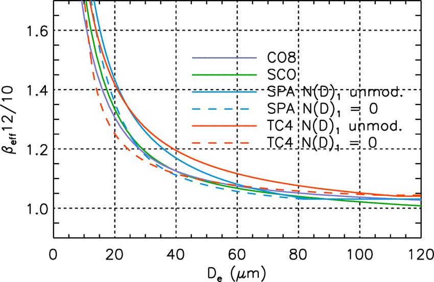
A. Garnier et al.: V4 IIR cloud microphysics: algorithms                                                                     3257

of an identical bias of dT12,BG = dTk,BG = +1 K in all the         sequently, the modeling of Earth surface radiance has been
channels. This positive bias increases εeff,12 ∼ 0 by ∼ 0.02       revisited in V4, as presented and evaluated in Sect. 3.3.
and has an insignificant impact at εeff,12 ∼ 1. Even though
the temperature bias is the same in all channels, 1εeff 12 − k     3.2.2    V3 biases at large emissivity
and βeff 12/k are also impacted: at εeff,12 ∼ 0.1 (or optical
depth ∼ 0.2, corresponding to a thin cirrus cloud), βeff 12/10     Large emissivities are typically found in so-called opaque
(dashed line) is decreased by 0.03 and βeff 12/08 (dashed–         clouds that fully attenuate the CALIOP signal. Importantly,
dotted line) by 0.06. The red curves illustrate the impact of      “opaque” means opaque to CALIOP, that is, cloud visible
a channel-dependent bias in TBG , by taking dT12,BG = 0 K          optical depth typically larger than 3 in V4 (Young et al.,
and dT10,BG = dT08,BG = +0.1 K. This modest inter-channel          2018) or effective emissivity expected to be larger than about
bias of dT12,BG − dTk,BG = −0.1 K induces a similar im-            0.8. In opaque ice clouds, V3 εeff,12 was rarely larger than
pact on both pairs of channels, with 1εeff 12 − k ∼ −0.002 at      0.95 (G12), and median 1εeff 12 − k was minimum around
εeff,12 ∼ 0 and βeff 12/k reduced by about 0.025 at εeff,12 ∼      εeff,12 = 0.95 rather than 1. Both suggested that εeff,12 was
0.1. Finally, the blue curves are obtained by taking an iden-      systematically too small and therefore that the cloud radia-
tical bias in all channels of dT12,BB = dTk,BB = +1 K. This        tive temperature was underestimated. In other words, obser-
increases εeff,12 ∼ 1 by ∼ 0.01 and has a negligible im-           vations in opaque ice clouds tended to be warmer than the
pact at εeff,12 ∼ 0. Again, this identical bias in all the chan-   computed blackbody temperatures by about 5 K (see Fig. 8
nels changes 1εeff 12 − k and βeff 12/k: at εeff,12 = 0.95,        in G12), while this systematic positive bias was not observed
βeff 12/10 is increased by 0.02 and βeff 12/08 by 0.03. As         for opaque warm water clouds. A similar contrast between
seen in Fig. 1c, an acceptable bias of, for instance, 0.02         ice and water clouds was also reported by Hu et al. (2010)
defines an emissivity domain of analysis ranging from 0.3          when comparing IIR observations and mid-cloud tempera-
to 0.9. This domain is mostly limited in the low emissivity        tures. Stubenrauch et al. (2010) reported that for high opaque
range, and refinements are necessary to extend this domain         ice clouds, the radiative height determined by the Atmo-
as much as possible.                                               spheric Infrared Sounder (AIRS) on board the Aqua satel-
                                                                   lite is on average lower than the altitude of the maximum
3.2     Motivations for changes in V4                              CALIOP 532 nm attenuated backscatter by about 10 % to
                                                                   20 % of the CALIOP apparent thickness. The warm bias be-
Changes in V4 were motivated by the need to reduce sys-            tween radiative temperature (Tr ) and the centroid tempera-
tematic errors in V3 microphysical retrievals that were made       ture Tc used in V3 was explained theoretically in G15. The
evident from statistical analyses of the IIR V3 products. Be-      Tr − Tc difference was found between 0 and +8 K for semi-
cause the sensitivity of the split-window technique decreases      transparent single-layered clouds and increased with cloud
as effective emissivity approaches 0 and 1, 1εeff 12 − k is        emissivity and geometric thickness, in agreement with previ-
supposed to tend towards zero on average when εeff,12 tends        ous studies (Stubenrauch et al., 2013, and references therein).
towards 0 and towards 1. Examining whether this behavior           Underestimating Tr (and therefore TOA TBB ) yields under-
was observed in our retrievals allowed us to identify errors       estimates in εeff,12 and the microphysical indices. Note that
related to the determination of background radiances when          Heidinger et al. (2010) infer cirrus radiative height from suit-
εeff,12 tended towards 0 and of blackbody radiances when           able pairs of channels using a range of expected values of
εeff,12 tended towards 1 (G13). These tests were paired with       βeff as a constraint. The problem here is reversed and is in-
comparisons between observed and modeled brightness tem-           stead to estimate Tr in order to infer microphysical indices.
peratures, whenever relevant.                                      The determination of Tr in ice clouds implemented in V4 is
                                                                   presented and discussed in Sect. 3.4.
3.2.1    V3 biases at small emissivity
                                                                   3.3     Background radiance from ocean surface in V4
Emissivity retrievals using Rk,BG observed in neighboring
pixels are a priori more robust than when this radiance is         3.3.1    FASRAD model
computed using a model. As discussed in G13, no biases
were detected in V3 in the former case. However, when the          The background radiance from the surface is computed using
ocean surface background radiances were computed using             the FASRAD model fed by horizontally and temporally inter-
the model, median 1εeff 12 − k at εeff,12 ∼ 0 was clearly neg-     polated temperature, water vapor, and ozone profiles and skin
ative, down to ∼ −0.015 for the 12–08 pair, which translated       temperatures. These ancillary data are from the MERRA-2
into significant low biases of the ice clouds microphysical in-    reanalysis products in V4. In V3, differences between ob-
dices at small emissivity (see Fig. 5 of G13 and Fig. 1c). This    served and computed brightness temperatures (BTDoc) in
was due to channel-dependent biases in the computed radi-          clear-sky conditions over oceans exhibited latitudinal and
ances, which could be assessed independently by comparing          seasonal variations for all channels (G12), which appeared
observations and computations in clear-sky conditions. Con-        to be related to variations in the water vapor profiles near

https://doi.org/10.5194/amt-14-3253-2021                                             Atmos. Meas. Tech., 14, 3253–3276, 2021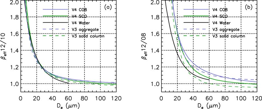
3258                                                                    A. Garnier et al.: V4 IIR cloud microphysics: algorithms

Figure 1. (a) Sensitivity of εeff,12 to systematic errors dT12,BG = +1 K (black), dT12,BG = 0 K (red, no error), and dT12,BB = +1 K (blue);
(b) sensitivity of 1εeff 12–10 (dashed lines) and 1εeff 12–08 (dashed–dotted lines) to systematic errors dT12,BG = dT10,BG = dT08,BG =
1 K (black), dT12,BG = 0 and dT10,BG = dT08,BG = 0.1 K (red), and dT12,BB = dT10,BB = dT08,BB = 1 K (blue). Panel (c) is the same as
panel (b) but for βeff 12/10 (dashed lines) and βeff 12/08 (dashed–dotted lines). Simulations using TBG = 285 K and TBB = 225 K, and
βeff 12/k = 1.1.

the surface to which the IIR window channels are the most               sis is plotted in Fig. 2b. Even though the ancillary data are
sensitive. The water vapor absorption coefficients were up-             from GMAO GEOS 5.10 in V3 for this time period and from
dated in V4, to take advantage of the advances in atmo-                 MERRA-2 in V4, the differences between V3 and V4 are
spheric spectroscopy over the last decade (Rothman et al.,              mostly due to the changes in the radiative transfer model. The
2013). Using MERRA-2 sea surface temperature and atmo-                  amplitude of the variations of median BTDoc with IWVP
spheric profiles, the model was tuned to minimize the resid-            is drastically reduced in V4 compared to V3 and the inter-
ual sensitivity of BTDoc to the column-integrated water va-             channel differences are significantly smaller. Between IWVP
por path (IWVP). This assessment was carried out in V4 pris-            of 1 and 5 g cm−2 , where most of the samples are found, V4
tine clear-sky conditions, i.e., when no layers were detected           median BTDoc is between −0.2 and 0.2 K for the three chan-
anywhere in the column or if the column included only low               nels. Using the V4 surface emissivities compensates for a
semi-transparent non-dust aerosols in which no single-shot              residual 10–12 inter-channel BTDoc bias of −0.15 K and a
cleared clouds were detected within the IIR pixel (Sect. 2).            residual bias of −0.3 K for the 08–12 pair. In contrast, the
Systematic biases remained for each channel, even at night              V3 median 10–12 and 08–12 inter-channel biases were up to
where the clear-sky mask is a priori the most accurate be-              −0.7 and −1.8 K, respectively, at IWVP of 5 g cm−2 .
cause of the increased CALIOP nighttime signal-to-noise
ratio. Nighttime BTDoc was on average equal to −0.5 K                   3.3.2   Evaluation vs. latitude and season
at 08.65 µm, −0.35 K at 10.6 µm, and −0.2 K at 12.05 µm.
These biases were explained by the combination of possible              In order to assess the errors in the computed background ra-
errors in the model, in the ancillary data, and in the calibra-         diances used in the effective emissivity retrievals (Rk,BG ; see
tion. We chose to reconcile observations and computations               Eq. 1) and in the corresponding computed brightness temper-
by using a new set of surface emissivity values (see Table 1)           atures (Tk,BG ), we analyzed distributions of BTDoc for dif-
with no attempt to include surface temperature variations as            ferent latitudes and seasons. Figures 3 and 4 show probability
reported from airborne measurements (Newman et al., 2005).              density functions (PDFs) of BTDoc at 12.05 µm, noted BT-
The derived surface emissivity values used in V4 are close to           Doc (12), and of the 10–12 and 08–12 inter-channel BTDoc
0.98 on average. It is noted that to save computation time, the         differences, noted BTDoc (10–12) and BTDoc (08–12), re-
contribution of the clear-sky downwelling radiance reflected            spectively. The results are for 2 months in opposite seasons,
by the surface is not included in the operational FASRAD                namely January 2008 (Fig. 3) and July 2006 (Fig. 4), with
model. Because the surface emissivity values are close to 1,            computations from V4 (solid lines) and from V3 (dashed
the subsequent impact on their derived values is not signifi-           lines). The data are split into four 30◦ latitude bands between
cant.                                                                   60◦ S and 60◦ N, for both night (blue) and day (red). Statis-
   As an illustration, median BTDoc is shown in Fig. 2a vs.             tics of the V4 differences (median, mean, standard deviation,
IWVP derived from MERRA-2 for each IIR channel, both                    and mean absolute deviation) are reported in Table 2 for the
in V4 (solid lines) and in V3 (dashed lines). Overplotted               four latitude bands and globally (i.e., 60◦ S–60◦ N).
in green is the median MERRA-2 sea surface temperature                     BTDoc (12) is overall less latitude dependent in V4 than
(Ts ). The results are shown for 6 months of nighttime data             in V3 due to the reduced bias related to IWVP in V4, and
in 2006 (from July through December) between 60◦ S and                  the width of the distributions is reduced. The V4 global stan-
60◦ N to ensure that the dataset is not contaminated by sea             dard deviations are similar for nighttime (0.8 K) and daytime
ice. The number of clear-sky IIR pixels used for this analy-            (0.9 K) data. Mean V4 BTDoc (12) is larger for daytime than

Atmos. Meas. Tech., 14, 3253–3276, 2021                                                   https://doi.org/10.5194/amt-14-3253-2021

A. Garnier et al.: V4 IIR cloud microphysics: algorithms                                                                             3259

Table 1. Surface emissivity over oceans in the three IIR channels in V3 and in V4.

                                                         Channel 08.65       Channel 10.6     Channel 12.05
                                Surface emissivity V3            0.9838              0.9906         0.9857
                                Surface emissivity V4             0.971               0.984          0.982

Figure 2. (a) Median difference between observed and computed brightness temperatures (BTDoc) at 08.65 µm (black), 10.6 µm (brown),
and 12.05 µm (red) vs. MERRA-2 IWVP in V4 pristine (no cleared clouds) nighttime clear-sky conditions in V4 (solid lines) and in V3
(dashed lines) over oceans between 60◦ S and 60◦ N from July through December 2006. The horizontal dotted lines denote the −0.2 and
+0.2 K limits. Overplotted in green is the median MERRA-2 surface temperature; (b) number of IIR pixels.

nighttime data at any latitude by 0.2 K on average. As men-               in each channel, the standard deviations around 0.31–0.35 K
tioned earlier, the V4 clear-sky mask is expected to be more              can be largely explained by the random noise in the observed
accurate at night than during the day. Undetected absorbing               temperatures, which is estimated to be 0.2–0.3 K. Thus, the
clouds would decrease the brightness temperature of the ob-               analysis of these inter-channel distributions shows that the
servations and therefore BTDoc (12), and a larger fraction                uncertainty in computed Tk,BG can be taken identical in all
of undetected clouds for daytime data would yield smaller                 channels. Based on the standard deviations in BTDoc (12),
daytime BTDoc (12) and not larger values as observed here.                the random error 1TBG is set to the conservative value ±1 K
A similar finding was reported in Garnier et al. (2017) for               for all channels.
both IIR and MODIS, suggesting that these differences are                    Again, the presence of clouds that were detected at single-
not due to calibration issues. The computations used a differ-            shot resolution and later cleared from the 5 km layer prod-
ent model, namely the 4A-OP radiative transfer model (Scott               uct is forbidden in the V4 clear-sky mask. The impact of
and Chédin, 1981), and ancillary data were from the ERA-                  this refinement in V4 is illustrated in Fig. 5, which com-
Interim reanalysis (Dee et al., 2011). It is unclear whether              pares the BTDoc histograms in V4, in which single-shot
the small but systematic day vs. night differences are due to             clouds are specifically excluded, and in pseudo-clear-sky
the V4 clear-sky mask or other reasons.                                   conditions (i.e., which contain at least one single-shot cloud)
   Again, the inter-channel differences are drastically re-               over oceans between 60◦ S and 60◦ N in January 2008. When
duced in V4 compared to V3, especially for the 08–12 pair                 cleared clouds are present (light blue and orange), median
of channels. In V4, the absolute values of the mean inter-                and mean BTDoc (12) are smaller by 1.3 and 2.2 K, respec-
channel differences are smaller than 0.1 K globally. The                  tively, and a marked negative tail down to about −8 K is ob-
worst cases are in July 2006 at 30–60◦ N (Fig. 4), where                  served, because these cleared clouds have a fairly large op-
mean BTDoc (10–12) and BTDoc (08–12) are equal to                         tical depth and are often colder than the surface. In this ex-
−0.15 and −0.26 K, respectively. The global standard devia-               ample, the fraction of IIR pixels that see at least one cleared
tions are around 0.31–0.35 K, notably smaller than 0.8–0.9 K              cloud in the column is 35 % at night and 22 % for daytime
found for BTDoc (12), because common biases due to errors                 data. The larger nighttime fraction is likely related to the fact
in sea surface temperature cancel out. Keeping in mind that               that the probability for CALIOP to detect a cloud at single-
the random noise at warm temperature is 0.15–0.2 K (G12)                  shot resolution is larger at night due to the larger daytime

https://doi.org/10.5194/amt-14-3253-2021                                                      Atmos. Meas. Tech., 14, 3253–3276, 2021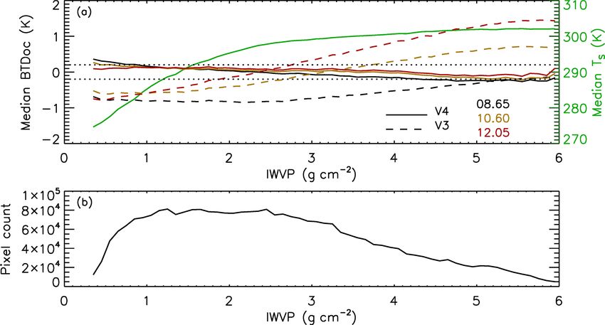
3260                                                                 A. Garnier et al.: V4 IIR cloud microphysics: algorithms

Table 2. V4 statistics (median, mean, standard deviation (SD), and mean absolute deviation (MAD)) of the differences between observed
and computed brightness temperatures in V4 clear-sky conditions (no cleared clouds) over oceans in January 2008 and in July 2006.

            January 2008     No. of IIR pixels              BTDoc (12) (K)     BTDoc (10–12) (K)     BTDoc (08–12) (K)
            Latitude band     Night       Day                Night      Day    Night          Day     Night         Day
            30–60◦ N         63 523     77 381    Median      0.15     0.15      0.03         0.02     0.03         0.05
                                                  Mean        0.19     0.00      0.04         0.03     0.07         0.09
                                                  SD          1.58     1.35      0.37         0.37     0.38         0.39
                                                  MAD         0.81     0.73      0.25         0.25     0.24         0.25
            0–30◦ N         156 987    195 197    Median    −0.02      0.09    −0.01        −0.01    −0.06        −0.10
                                                  Mean      −0.06      0.00    −0.01        −0.01    −0.05        −0.09
                                                  SD         0.75      0.80     0.30         0.31     0.32         0.33
                                                  MAD        0.53      0.57     0.23         0.23     0.24         0.25
            0–30◦ S         178 318    258 476    Median     0.02      0.31    −0.05          0.02   −0.11        −0.08
                                                  Mean      −0.03      0.23    −0.05         0.023   −0.10        −0.07
                                                  SD         0.64      0.80     0.29          0.31    0.31         0.34
                                                  MAD        0.47      0.54     0.22          0.22    0.23         0.25
            30–60◦ S        157 130    234 098    Median      0.26     0.56    −0.04          0.00   −0.06        −0.06
                                                  Mean        0.22     0.51    −0.04          0.01   −0.06        −0.05
                                                  SD          0.69     0.91     0.29          0.30    0.30         0.30
                                                  MAD         0.49     0.59     0.21          0.22    0.21         0.22
            60◦ S–60◦ N     555 958    765 152    Median      0.09     0.31    −0.03          0.01   −0.07        −0.06
                                                  Mean        0.05     0.23    −0.02          0.01   −0.06        −0.05
                                                  SD          0.85     0.93     0.31          0.31    0.32         0.34
                                                  MAD         0.54     0.60     0.23          0.23    0.23         0.24
            July 2006        No. of IIR pixels                BTDoc (12)         BTDoc (10–12)         BTDoc (08–12)
            Latitude band     Night       Day                Night      Day    Night          Day     Night         Day
            30–60◦ N         52 481     79 420    Median      0.15     0.46    −0.04        −0.04    −0.13        −0.24
                                                  Mean        0.19     0.38    −0.04        −0.06    −0.15        −0.26
                                                  SD          0.97     1.27     0.31         0.35     0.35         0.34
                                                  MAD         0.66     0.75     0.23         0.24     0.26         0.26
            0–30◦ N          71 144    103 625    Median    −0.06      0.17    −0.05          0.00   −0.13        −0.12
                                                  Mean       −0.1      0.10    −0.05          0.00   −0.13        −0.11
                                                  SD         0.67      0.79     0.29          0.31    0.32         0.34
                                                  MAD         0.5      0.55     0.22          0.23    0.25         0.26
            0–30◦ S         169 803    213 552    Median      0.06     0.20    −0.03        −0.03    −0.06        −0.05
                                                  Mean        0.01     0.13    −0.03        −0.03    −0.05        −0.05
                                                  SD          0.69     0.72     0.30         0.30     0.32         0.32
                                                  MAD         0.48     0.51     0.22         0.22     0.24         0.24
            30–60◦ S         93 935    108 760    Median      0.14     0.24      0.01         0.00     0.08         0.04
                                                  Mean        0.06     0.14      0.02         0.01     0.08         0.06
                                                  SD          0.83     0.82      0.36         0.36     0.36         0.35
                                                  MAD         0.54     0.54      0.25         0.25     0.24         0.24
            60◦ S–60◦ N     387 363    505 357    Median      0.06     0.24    −0.03        −0.02    −0.05        −0.07
                                                  Mean        0.03     0.16    −0.02        −0.02    −0.05        −0.07
                                                  SD          0.77     0.87     0.32         0.33     0.35         0.35
                                                  MAD         0.53     0.57     0.23         0.23     0.25         0.26

Atmos. Meas. Tech., 14, 3253–3276, 2021                                                 https://doi.org/10.5194/amt-14-3253-2021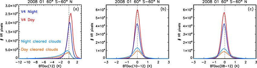
A. Garnier et al.: V4 IIR cloud microphysics: algorithms                                                                               3261

Figure 3. Probability density functions (PDFs) of the differences between observed and computed brightness temperatures (BTDoc) over
oceans in January 2008 in V4 pristine (no cleared clouds) nighttime (blue) and daytime (red) clear-sky conditions in V4 (solid lines) and
in V3 (dashed lines). Panels (a), (d), (g), (j): BTDoc at 12.05 µm. Panels (b), (e), (h), (k): 10–12 inter-channel BTDoc difference. Panels
(c), (f), (i), (l): 08–12 inter-channel BTDoc difference. The PDFs are shown at 30–60◦ N (a, b, c), 0–30◦ N (d, e, f), 30–0◦ S (g, h, i), and
60–30◦ S (j, k, l).

background noise, so the probability that these clouds are               layers, noted T 2 overlying . Following the rationale presented in
cleared from the product is larger at night. The mean and me-            Appendix B, the centroid altitude of a multi-layer cloud sys-
dian values of the inter-channel BTDoc are barely impacted,              tem composed of N layers is computed as
showing that the cleared clouds induce a similar bias in the                   Pl=N
three IIR channels.                                                                    Zc (l) · IAB(l) · T 2 overlying (l)
                                                                         Zc = l=1  Pl=N                                    .            (4)
                                                                                                        2
                                                                                      l=1 IAB(l) · T overlying (l)
3.4     Radiative temperature in V4
                                                                         For single-layer cases (N = 1), Zc is obviously the centroid
3.4.1    Centroid altitude and temperature                               altitude reported in the CALIOP data product. For multi-
                                                                         layer cases, the cloud system is seen as an equivalent sin-
Both in V3 and in V4, the first step into the computation of             gle layer characterized by Zc given in Eq. (4), whose top
the radiative temperature is to determine the centroid alti-             and base altitudes are the top of the uppermost layer and the
tude, Zc , of the cloud system. The centroid altitude of each            base of the lowermost layer, respectively. The approach is
layer is reported in the CALIOP 5 km layer product, together             the same as that in V3, except that, because of an error in
with the 532 nm integrated attenuated backscatter (hereafter             the computation of T 2 overlying in the V3 IIR algorithm, esti-
IAB) of each layer. IAB is corrected for the molecular con-              mates of Zc could be too low by up to several kilometers in
tribution and for the attenuation resulting from the overlying           V3 multi-layer cases.

https://doi.org/10.5194/amt-14-3253-2021                                                    Atmos. Meas. Tech., 14, 3253–3276, 2021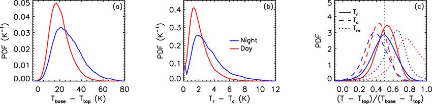
3262 A. Garnier et al.: V4 IIR cloud microphysics: algorithms
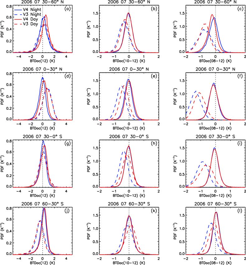
Figure 4. Same as Fig. 3 but for July 2006.
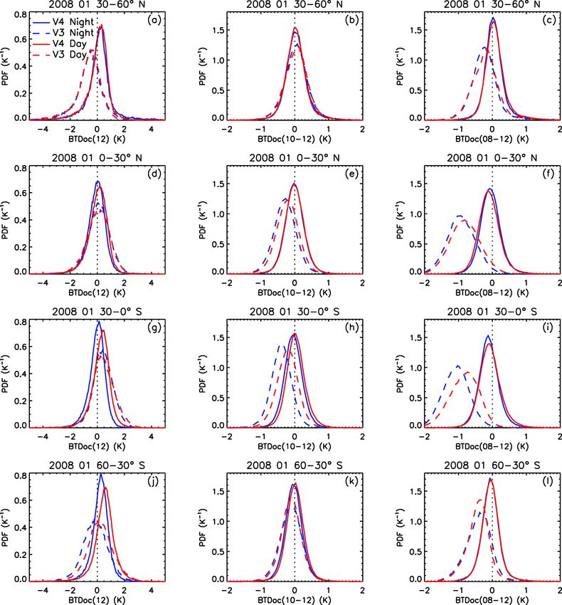
Figure 5. Histograms of the differences between observed and computed brightness temperatures over oceans between 60◦ S and 60◦ N in
January 2008 in V4 clear-sky conditions (no cleared clouds) (navy blue: night; red: day) and in pseudo-clear-sky conditions (cleared clouds
in the column) (light blue: night; orange: day). (a) BTDoc at 12.05 µm; (b) 10–12 and (c) 08–12 inter-channel BTDoc differences.
In V3, the radiative temperature (Tr ) was set to the centroid 3.4.2 Radiative temperature in ice clouds
temperature (Tc ) for any cloud system. The approach is the
same in V4, except when all the layers are classified as ice As demonstrated in G15, the radiative temperature Tr (k) in
by the V4 ice–water phase algorithm (Avery et al., 2020). channel k is the brightness temperature associated with the
In the latter case, Tr is derived from Tc and parameterized centroid radiance of the attenuated infrared emissivity pro-
functions, as presented and illustrated in the next section. file within the cloud. For a cloud containing a number, n, of
vertical bins, i, of resolution δz, with i = 1 to i = n from base
to top, this centroid radiance can be written as a function of
Atmos. Meas. Tech., 14, 3253–3276, 2021 https://doi.org/10.5194/amt-14-3253-2021A. Garnier et al.: V4 IIR cloud microphysics: algorithms 3263
radiance Rk (i) of bin i and CALIOP particulate (i.e., cloud) the range of temperature-dependent values used in V4 (G15;
extinction coefficient, αpart (i), as Young et al., 2018). Variations with η were not discussed in
G15 because η was taken constant and equal to 0.6 in V3.
Pj =n+1
Pi=n
1 − e− αpart (i) · δz/r · Rk (i).e j =i+1 [ part
− α (j )·δz/r ] The Tr (k) − Tc differences were examined against the
i=1
Rk = . “thermal thickness” of the clouds, that is, the difference be-
εeff,k
tween the temperatures at cloud base (Tbase ) and at cloud top
(5)
(Ttop ). Overall, 90 % of the CALIOP profiles used for this
The term αpart (i) · δz/r in Eq. (5) is the absorption optical analysis had Tbase − Ttop between 10 and 50 K. The median
depth in bin i. The ratio, r, of CALIOP optical depth to IIR relative difference (Tr − Tc )/(Tbase − Ttop ) was found to vary
absorption optical depth is taken equal to 2 (G15). The radi- linearly with Tbase − Ttop , as illustrated in Fig. 6a for channel
ance Rk (i) is determined from the thermodynamic tempera- 12.05 µm using η = 0.6. Figure 6b and c show that the in-
ture in bin i. tercepts (a0 ) and the slopes (a1 ) of the regression lines vary
On the other hand, Tc is the temperature at the centroid with cloud absorption optical depth τa,12 . Furthermore, the
altitude of the attenuated 532 nm backscatter coefficient pro- Tr − Tc differences increase with η because the CALIOP sig-
file, which is written as a function of altitude Z(i) of bin i nal is attenuated more quickly when less multiple scattering
and αpart (i) as (i. e., larger η) contributes to the backscattered signal. As a
result, both a0 (Fig. 6b) and a1 (Fig. 6c) increase as η is in-
Pj =n creased from 0.5 to 0.8. Finally, the mathematical expression
βpart (i) + βmol (i) · e−2 j =i [ηαpart (j )+αmol (j )]·δz
Pi=n
i=1 Z(i) · for the correction implemented in V4 is
Zc = Pj =n .
βpart (i) + βmol (i) · e−2 j =i [ηαpart (j )+αmol (j )]·δz
Pi=n
i=1
Tr (k) − Tc = a0 τa,k , η, k × Tbase − Ttop
(6)
2
+ a1 τa,k , η, k × Tbase − Ttop , (7)
In Eq. (6), βpart (i) is the cloud particulate backscatter in bin
i, αmol (i) and βmol (i) are the molecular extinction coefficient where the letter k refers to the IIR channel. The corrections
and backscatter, respectively, and η is the ice cloud multiple derived from Fig. 6a are shown in Fig. 6d. For a given value
scattering correction factor (Young et al., 2018, and refer- of Tbase − Ttop , Tr − Tc increases with εeff,12 until εeff,12 =
ences therein). 0.7–0.8 and is maximum for εeff,12 = 0.8–0.99 (or τa,12 be-
Using V3 CALIOP extinction and backscatter profiles in tween 1.6 and 4.6), where it represents 10 % to 25 % of the
semi-transparent ice clouds, the Tr − Tc difference was found cloud thermal thickness. We find that Tr (k) is slightly larger
to increase with both cloud optical depth and geometric at 10.6 µm than at 12.05 µm, by less than 0.3 K in the worst
thickness (G15). case, and somewhat larger at 08.65 µm than at 12.05 µm but
Because the CALIOP extinction profiles are not used in always by less than 1 K (not shown). Because at this stage of
the IIR operational algorithm, the approach in V4 was to the algorithm, the final value of τa,k is still unknown, τa,k in
establish parameterized correction functions, Tr (k) − Tc , for Eq. (7) is the initial V3 value derived by taking Tr = Tc . No
each channel k, and to correct the initial estimate Tc that correction is applied when the initial emissivity is found to
was used in V3 as Tr (k) = Tc +[Tr (k)−Tc ]. These correction be larger than 1.
functions were derived offline from the statistical analysis The errors in the ice cloud radiative temperature correc-
of a series of simulated extinction and attenuated backscat- tions were assessed by comparing Tr derived directly using
ter profiles. In order to reproduce the variability associated the CALIOP extinction profiles with Tr derived from Eq. (7).
with the various possible shapes of the extinction profiles, we The statistics obtained from the same 8000 CALIOP profiles
chose to use actual V4 CALIOP profiles (8000 profiles were as above are provided in Table 3, for both the Tr − Tc cor-
used) rather than synthetic profiles. These initial CALIOP rection and the correction error, for channel 12.05 µm. These
profiles were derived from single-layered semi-transparent statistics are provided for εeff,12 equal to 0.2, 0.6, and 0.99,
clouds classified with high confidence as randomly oriented and using η equal to the extreme values 0.5 and 0.8. The me-
ice (ROI) by the V4 ice–water phase algorithm (Avery et dian and mean correction errors are smaller than 0.25 K and
al., 2020). Each CALIOP extinction (and backscatter) profile significantly smaller than the median and mean corrections,
was scaled to simulate several pre-defined optical depths cor- which are found between 0.8 and 5 K. The standard devi-
responding to several pre-defined effective emissivities using ations of the correction errors are between 0.66 and 1.2 K
r = 2, and the attenuated backscatter profile was simulated at η = 0.5 and between 0.7 and 1.75 K at η = 0.8, while
by applying the required attenuation to the simulated total their mean absolute deviations are smaller than 1.25 K. These
(molecular and particulate) backscatter profile. The simula- quantities represent the estimated random error in the cloud
tions of Tr (k) using Eq. (5) and of Tc using Eq. (6) were radiative temperature correction resulting from the variabil-
carried out for εeff,k ranging between 0.1 (or τa,k = 0.1; see ity in the shape of the extinction profiles.
Eq. 2) and 0.99 (or τa,k = 4.6). Variations of Tr (k) − Tc with Again, the maximum corrections are for clouds having ini-
η between 0.5 and 0.8 were also analyzed in order to cover tial effective emissivities in the 0.8–0.99 range and are simi-
https://doi.org/10.5194/amt-14-3253-2021 Atmos. Meas. Tech., 14, 3253–3276, 20213264 A. Garnier et al.: V4 IIR cloud microphysics: algorithms
Figure 6. V4 correction functions of ice cloud radiative temperature: (a) (Tr − Tc ) / (Tbase − Ttop ) vs. Tbase − Ttop for effective emissivities
between 0.1 and 0.99 and η = 0.6. The solid lines are median values from statistical analyses and the dashed lines are regression lines; (b)
intercept and (c) slope of the regression lines vs. τa,12 for η between 0.5 and 0.8; (d) resulting V4 corrections Tr − Tc vs. Tbase − Ttop for
effective emissivities between 0.1 and 0.99 and η = 0.6. Results are for channel 12.05 µm.
Table 3. Statistics (median, mean, standard deviation (SD), and mean absolute deviation (MAD)) of the Tr − Tc correction at 12.05 µm and
of correction errors for εeff,12 equal to 0.2, 0.6, and 0.99, using η equal to 0.5 and 0.8.
Tr − Tc correction (K) Correction error (K)
εeff,12 = 0.2 εeff,12 = 0.6 εeff,12 = 0.99 εeff,12 = 0.2 εeff,12 = 0.6 εeff,12 = 0.99
η = 0.5 Median 0.81 2.04 3.07 0.08 −0.01 0.01
Mean 0.92 2.22 3.43 0.1 0.02 0.13
SD 0.55 1.16 1.98 0.66 0.75 1.2
MAD 0.43 0.93 1.56 0.46 0.53 0.84
η = 0.8 Median 1.32 3.8 4.50 0.17 −0.01 0.01
Mean 1.45 4.11 5.01 0.23 0.00 0.17
SD 0.78 2.08 2.86 0.7 0.98 1.74
MAD 0.62 1.65 2.26 0.50 0.70 1.24
lar for emissivities larger than 0.9. This range of initial emis- Consequently, both Tc and Tr are a priori more accurate at
sivities is found for clouds that are opaque to CALIOP. It night. Figure 7c shows the Tr −Ttop (solid lines) and Tc −Ttop
is noted that the corrections are a priori underestimated for (dashed lines) differences relative to the apparent Tbase −Ttop .
opaque clouds. Because the CALIOP signal does not pen- After correction, the nighttime mean ± standard deviation of
etrate to the true base of opaque layers, the reported base (Tr − Ttop ) / (Tbase − Ttop ) is 0.48 ± 0.15. This result is fully
is instead an apparent one, and so Tbase –Ttop is a priori too consistent with Stubenrauch et al. (2017), who report that the
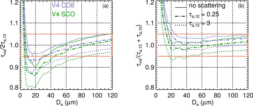
small. Figure 7 illustrates the impact of the correction ap- radiative cloud height derived from AIRS is, on average, at
plied to V4 opaque ice clouds classified as high-confidence mid-distance between the CALIOP cloud top and cloud ap-
ROIs for IIR channel 12.05. The apparent thermal thickness parent base in high opaque clouds at night. Because the IR
(Fig. 7a) is larger at night (blue) compared to day (red), as absorption above ice clouds is usually weak, Tr is close to
already mentioned in Young et al. (2018). In this example, TOA TBB . For reference, the dotted lines in Fig. 7c represent
nighttime and daytime mean ± standard deviation of Tbase – (Tm − Ttop ) / (Tbase − Ttop ), where Tm is the measured bright-
Ttop are 28 ± 13 K and 21 ± 9 K, respectively. Similarly, the ness temperature (here T12,m ). Tm represents the warmest
Tr − Tc corrections shown in Fig. 7b are larger at night. The possible value for TBB ∼ Tr if all clouds had effective emis-
discontinuities around Tr − Tc = 0 in Fig. 7b are due to pix- sivity equal to unity. At night, Tm is always located within the
els with initial emissivity larger than 1 for which no correc- apparent cloud, at 61 % from the top as compared to 48 % for
tion is applied, which occurs more often at night. The smaller Tr . The Tm − Tr difference represents the maximum possible
daytime apparent thickness is explained by the larger back- bias in the estimation of Tr and is equal to 1.5 K on average.
ground noise in CALIOP daytime measurements, which in- For daytime data, both Tr and Tm are lower in the apparent
creases the difficulty in accurately locating cloud boundaries. cloud than at night, and even below (Tm >Tbase ), which is at
Atmos. Meas. Tech., 14, 3253–3276, 2021 https://doi.org/10.5194/amt-14-3253-2021A. Garnier et al.: V4 IIR cloud microphysics: algorithms 3265
least in part due to the smaller daytime apparent thickness. 4.1 V4 look-up tables
Further evaluation will be carried out in the future using ex-
tinction profiles and true cloud base altitudes derived from The difference between the V4 and the V3 ice LUTs is two-
the CloudSat radar. fold: the ice habit models are different and a particle size
With the introduction of corrections to the cloud radiative distribution (PSD) is introduced in V4. Three ice habit mod-
temperatures for ice clouds, V4 emissivities and microphys- els were used in V3. These were taken from the database
ical indices now depend on the CALIOP ice–water phase described in Yang et al. (2005) and represented three fami-
classification. However, for optically very thin ice clouds, lies of relationships between βeff 12/10 and βeff 12/08: solid
the corrections are typically smaller than 1 K, and, further- column, aggregate, and plate (G13). In practice, the plate
more, these small corrections induce little changes in the final model was rarely selected by the algorithm. In V4, the LUTs
effective emissivity and microphysical indices (see Fig. 1). are computed using state-of-the-art ice crystal properties re-
Thus, microphysical indices can be considered independent ferred to as “TAMUice2016” by Bi and Yang (2017), which
of the CALIOP ice–water phase at small emissivities, typi- were updated with respect to TAMUice2013 reported in 2013
cally smaller than 0.3. (Yang et al., 2013). These optical properties determined by
the Texas A&M University group are now widely used by
3.4.3 Radiative temperature in liquid water clouds the scientific community (Yang et al., 2018). Two models
are used in V4: severely roughened “eight-element column
In the case of opaque liquid water clouds, the observed aggregate” (hereafter CO8) and “single hexagonal column”
brightness temperature (Tm ) is, on average, close to the TOA (hereafter SCO), for which the degree of the particle’s sur-
TBB inferred from Tc . This indicates that the temperature at face roughness has little impact on the IIR channels. The for-
the centroid altitude is a good proxy for Tr , which is why no mer is the MODIS Collection 6 ice model for retrievals in the
change was implemented in the V4 algorithm for liquid wa- visible–near-infrared spectral domain (except that the choice
ter clouds. Nevertheless, significant differences between V4 of the MODIS model was based on TAMUice2013 proper-
and V3 can arise from differences in the meteorological data. ties), where the so-called “bulk” optical properties are com-
This is illustrated in Fig. 8, which shows PDFs of Tm − TBB puted using a gamma PSD with an effective variance of 0.1
at 12.05 µm in V4 (solid lines) and in V3 (dashed lines) for (Hansen, 1971; Baum et al., 2011; Platnick et al., 2017). The
opaque water clouds having identical centroid altitudes in V3 same gamma PSD is chosen to compute the V4 IIR LUTs,
and in V4. These clouds are classified as water with high con- whereas no PSD was introduced in V3 (G13).
fidence by the V4 ice–water phase algorithm and they are the For retrievals in liquid water clouds, which were added in
only layer detected in the column. The V3 − V4 differences V4, the LUTs are computed using the Lorenz–Mie theory
are due mainly to the different temperature profiles (GMAO with refractive indices from Hale and Querry (1973) and us-
GEOS 5.10 in V3 and MERRA-2 in V4), yielding differ- ing the same PSD as for ice clouds.
ent values of Tc for an identical centroid altitude, and to a As in V3, the LUTs are established for several values
smaller extent to the changes in the water vapor profiles and of εeff,12 (G13). Shown in Fig. 9 are the V4 (solid lines)
in the FASRAD model. The V4 differences are −0.6 ± 2.2 K and V3 (dashed lines) LUTs computed for εeff,12 = 0.23
at night and 0.12 ± 2.7 during the day. The larger fraction (visible optical depth ∼ 0.5). This figure highlights that the
of negative Tm − TBB differences in V3, from −2 down to βeff 12/k microphysical indices are very sensitive to the pres-
−10 K, has been traced back to cases with strong tempera- ence of small particles in the PSD (Mitchell et al., 2010), with
ture inversions near the top of the opaque cloud, which seem βeff 12/k decreasing rapidly as De increases up to 50 µm and
to be better reproduced in MERRA-2. then tending asymptotically to ∼ 1 at the upper limit of the
sensitivity range; that is, De = 120 µm for ice crystals and
4 Effective diameter 60 µm for liquid droplets. The retrieval of large particle sizes
becomes very sensitive to noise and biases in the microphys-
The βeff 12/k microphysical indices (Eq. 3) are interpreted ical indices. In V4, the LUTs are extended to De = 200 µm
in terms of ice crystal or liquid droplet effective diameter for ice clouds and 100 µm for water clouds. Doing this al-
using LUTs built with the FASDOM model (Dubuisson et lows the user to perform dedicated analyses when β12/k is
al., 2008) and available optical properties (G13). Following only slightly smaller than the lower sensitivity limit, but De
Foot (1988) and Mitchell (2002), the effective diameter is retrievals beyond the sensitivity limit are very uncertain and
defined as flagged accordingly.
For ice clouds, the V4 βeff 12/10–De relationships are
3 V relatively insensitive to the crystal model compared to the
De = × , (8)
2 A βeff 12/08 − De ones, due to the larger single scattering
where V and A are the total volume and the projected area albedo at 08.65 µm. The model dependence of the βeff 12/10–
that are integrated over the size distribution, respectively. βeff 12/08 relationship is used as a piece of information about
the ice model and the shape of the ice crystals to ulti-
https://doi.org/10.5194/amt-14-3253-2021 Atmos. Meas. Tech., 14, 3253–3276, 2021You can also read