Virtual Platform for Reinforcement Learning Research for Heavy Vehicles
←
→
Page content transcription
If your browser does not render page correctly, please read the page content below
DF

Virtual Platform for Reinforcement
Learning Research for Heavy Vehicles
Implementing reinforcement learning in a open-source vehicle
simulation model
Bachelor’s thesis in Mechanical Engineering

CARL EMVIN
JESPER PERSSON
WILLIAM ÅKVIST

Department of Mechanics and Maritime Sciences
C HALMERS U NIVERSITY OF T ECHNOLOGY
Gothenburg, Sweden 2020
BACHELOR’S THESIS 2020:02

     Virtual Platform for Reinforcement
    Learning Research for Heavy Vehicles

Implementing reinforcement learning in a open-source vehicle
                     simulation model

CARL EMVIN, JESPER PERSSON & WILLIAM ÅKVIST

                                     DF

         Department of of Mechanics and Maritime Sciences
           Vehicle Engineering and Autonomous Systems
            Chalmers University of Technology
                    Gothenburg, Sweden 2020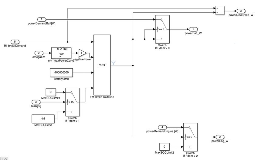
Virtual Platform for Reinforcement Learning Research for Heavy Vehi-
cles
Implementing reinforcement learning in a open-source vehicle simulation model
C. EMVIN, J. PERSSON, W. ÅKVIST

© C.EMVIN, J. PERSSON, W. ÅKVIST, 2020.

Supervisor: Luigi Romano, Department of Mechanics and Maritime Sciences, Chalmers
University of Technology
Examiner: Prof. Bengt J H Jacobson, Department of Mechanics and Maritime
Sciences, Chalmers University of Technology

Bachelor’s thesis 2020:02
Department of Mechanics and Maritime Sciences
Vehicle Engineering and Autonomous Systems
Chalmers University of Technology
SE-412 96 Gothenburg
Telephone +46 31 772 1000

Cover: Environment, driver and vehicle in Volvo’s Global Simulation Platform.

Typeset in LATEX, template by David Frisk
Printed by Chalmers Reproservice
Gothenburg, Sweden 2020

iv
Virtual Platform for Reinforcement Learning Research for Heavy Vehicles
Implementing reinforcement learning in a open-source vehicle simulation model
C. EMVIN, J. PERSSON, W. ÅKVIST
Department of Mechanics and Maritime Sciences
Chalmers University of Technology

Abstract
The main objective of the project, tasked by Volvo Group Trucks Technology, is to
implement a reinforcement learning agent in a open-source vehicle simulation model
known as VehProp, developed at Chalmers University of Technology in MathWorks
Simulink. The project also aims to improve VehProp, particularly the Equivalent
Consumption Minimization Strategy. As a proof of concept for the reinforcement
learning implementation, an agent is trained to control the brakes of a hybrid elec-
tric heavy duty vehicle in order to minimize fuel consumption through regenerative
braking. Much effort is put in the theory chapter, explaining reinforcement learning
and the simulation platform. The reinforcement learning agent is successfully im-
plemented in the simulation platform, using the Reinforcement Learning Toolbox in
Matlab. The training of the agent to control the brakes of a hybrid electric heavy
duty vehicle was unsuccessful, with the agent failing to display the wanted behav-
ior. Suggestions for future work with the agent are presented, mainly fulfilling the
Markov property, investigating sparse reward functions and the general implementa-
tion of the agent to assure action-reward causality. Improvements to the Equivalent
Consumption Minimization Strategy of the simulation platform were made with a
decrease in fuel consumption as a result.

Keywords: reinforcement learning, vehicle simulation, VehProp, hybrid electric ve-
hicle.

                                                                                  v
Acknowledgements
Thank you to Rickard Andersson for offering the oppurtunity to collaborate with
Volvo GTT and providing a steady stream of ideas for improvement of VehProp;
Mikael Enelund for his interest in our work and his commitment to Global Capstone
projects at Chalmers; Luigi Romano for his involvement in the project as supervisor
and Constantin Cronrath for introducing us to the field of reinforcement learning
and providing technical advice.
This paper is part of a Global Capstone project, a joint student project between
Chalmers University of Technology and Pennsylvania State University. The authors
would like to acknowledge the Penn State students: Jackie Cheung, Ashley Gal-
lagher, Cheng Li and Joshua Nolf, and thank them for their hospitality during the
Chalmers team’s visit to State College, PA.
A special thank you to Herbert & Karin Jacobssons Stiftelse for funding the team’s
trip to the US.
William Åkvist, Carl Emvin, Jesper Persson, Gothenburg, May 2020
viAbbreviations
ECMS Equivalent Consumption Minimization Strategy
EM Electric Motor
GSP Global Simulation Platform
ICE Internal Combustion Engine
MDP Markov Decision Process
PPO Proximal Policy Optimization
RL Reinforcement Learning
SOC State Of Charge
TRPO Trust Region Policy Optimization
viiContents
1 Introduction 1
1.1 Background . . . . . . . . . . . . . . . . . . . . . . . . . . . . . . . . 1
1.2 Objectives . . . . . . . . . . . . . . . . . . . . . . . . . . . . . . . . . 2
1.2.1 Client needs . . . . . . . . . . . . . . . . . . . . . . . . . . . . 3
1.2.2 Deliverables . . . . . . . . . . . . . . . . . . . . . . . . . . . . 3
1.2.3 Delimitations . . . . . . . . . . . . . . . . . . . . . . . . . . . 4
1.3 Considerations . . . . . . . . . . . . . . . . . . . . . . . . . . . . . . 4
1.3.1 Ethical statement . . . . . . . . . . . . . . . . . . . . . . . . . 5
1.3.2 Environmental statement . . . . . . . . . . . . . . . . . . . . . 5
2 Theory 6
2.1 Reinforcement learning . . . . . . . . . . . . . . . . . . . . . . . . . . 6
2.1.1 Markov decision processes . . . . . . . . . . . . . . . . . . . . 7
2.1.2 Value functions . . . . . . . . . . . . . . . . . . . . . . . . . . 7
2.1.3 Reinforcement learning algorithms . . . . . . . . . . . . . . . . 8
2.1.4 Problems with reinforcement learning . . . . . . . . . . . . . . 9
2.2 VehProp . . . . . . . . . . . . . . . . . . . . . . . . . . . . . . . . . . 9
2.2.1 Simulation type . . . . . . . . . . . . . . . . . . . . . . . . . . 9
2.2.2 Structure . . . . . . . . . . . . . . . . . . . . . . . . . . . . . 10
2.2.2.1 Operating cycle . . . . . . . . . . . . . . . . . . . . . 10
2.2.2.2 Driver . . . . . . . . . . . . . . . . . . . . . . . . . . 10
2.2.2.3 Vehicle . . . . . . . . . . . . . . . . . . . . . . . . . 10
2.3 Global Simulation Platform . . . . . . . . . . . . . . . . . . . . . . . 12
2.4 QSS Toolbox . . . . . . . . . . . . . . . . . . . . . . . . . . . . . . . 12
2.5 Reinforcement Learning Toolbox . . . . . . . . . . . . . . . . . . . . . 13
2.5.1 Agent block . . . . . . . . . . . . . . . . . . . . . . . . . . . . 13
2.5.2 Creating agent environment . . . . . . . . . . . . . . . . . . . 14
2.5.3 Creating PPO agent . . . . . . . . . . . . . . . . . . . . . . . 14
2.5.4 Training agent . . . . . . . . . . . . . . . . . . . . . . . . . . . 15
3 Methods 16
3.1 Implementation of an RL controller in VehProp using Reinforcement
Learning Toolbox . . . . . . . . . . . . . . . . . . . . . . . . . . . . . 16
3.1.1 RL agent block . . . . . . . . . . . . . . . . . . . . . . . . . . 16
3.1.2 Driver/RL agent interaction . . . . . . . . . . . . . . . . . . . 17
3.2 Verification of VehProp . . . . . . . . . . . . . . . . . . . . . . . . . . 18
viiiContents
3.3 RL agent setup . . . . . . . . . . . . . . . . . . . . . . . . . . . . . . 19
3.3.1 Agent options . . . . . . . . . . . . . . . . . . . . . . . . . . . 19
3.3.2 Training options . . . . . . . . . . . . . . . . . . . . . . . . . 20
3.3.3 Training process . . . . . . . . . . . . . . . . . . . . . . . . . . 20
3.4 Reward function . . . . . . . . . . . . . . . . . . . . . . . . . . . . . . 21
3.5 Improving ECMS in VehProp . . . . . . . . . . . . . . . . . . . . . . 22
4 Results 24
4.1 Agent convergence . . . . . . . . . . . . . . . . . . . . . . . . . . . . 24
4.2 Vehicle speed . . . . . . . . . . . . . . . . . . . . . . . . . . . . . . . 25
4.3 Improvement of braking using RL . . . . . . . . . . . . . . . . . . . . 28
4.4 Improvement of ECMS in VehProp . . . . . . . . . . . . . . . . . . . 28
4.5 Verification of VehProp . . . . . . . . . . . . . . . . . . . . . . . . . . 30
5 Conclusion 31
5.1 Conclusion . . . . . . . . . . . . . . . . . . . . . . . . . . . . . . . . . 31
5.2 Future work . . . . . . . . . . . . . . . . . . . . . . . . . . . . . . . . 31
Bibliography 33
ix1
Introduction
Hybrid vehicles are becoming evermore popular, filling the need for transport with
less emission. When vehicles become more complex the need for testing in a virtual
environment becomes greater as well as the complexity of controlling the vehicles
many different features.
One way to handle the increasing complexity of heavy vehicles is to simulate the
vehicle in a virtual simulation platform by incorporating machine learning. More
specifically, reinforcement learning (RL), which shows a great deal of promise. By
developing an open-source virtual simulation platform, the possibilities for rapid
testing and prototyping of experimental RL controllers are increased, and the coop-
eration between industry parties and academia can be enriched.
1.1 Background
Volvo Group Trucks Technology (Volvo GTT) has teamed up with Chalmers Uni-
versity of Technology and Pennsylvania State University to incorporate RL in an
open-source virtual simulation platform called VehProp, the platform has been de-
veloped at Chalmers for the simulation of heavy duty vehicles. An established route,
depicted in figure 1.1, is used to test the RL implementation.
Figure 1.1: Route driven from Viared, Borås to Gothenburg harbor.
This route, a total distance from start to finish of 152.6 km, connects Gothenburg
Harbor to Viared Borås in Sweden. Over the course of the route, the altitude varies,
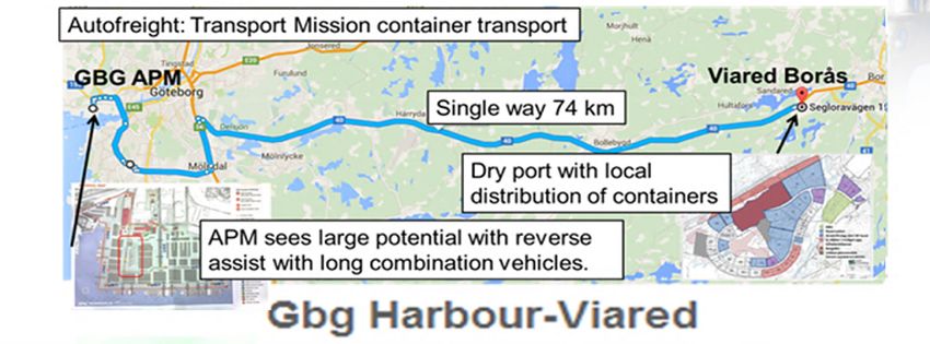
11. Introduction ranging from about 40 meters to 220 meters. Volvo GTT presents the task of emu- lating the route in Sweden using VehProp and implement an RL agent for controlling the use of electrical motor (EM) brakes as a proof of concept for the platform. Volvo currently uses a simulation platform called the Global Simulation Platform (GSP) that “enables the development and verification of advanced controllers. A truck can be built and then driven on a virtual road”. This platform is used to test the heavy duty vehicles in a virtual environment before they are tested on the real route. The reason for using VehProp rather than developing GSP further is the need for an open-source virtual simulation platform which can be shared with Volvo’s external partners, e.g. Chalmers students and researchers as well as industry parties. By simulating the trucks on the virtual platform with the incorporation of the RL module, the usage of the service brakes can be reduced, thus increasing the amount of regenerative braking by using the EM brakes. This will increase the overall fuel efficiency of the vehicle. 1.2 Objectives The overall objective for the project is to deliver a virtual platform suitable for RL applications in vehicles, which can be shared externally between partners and sup- pliers. The objective also includes creating a basis for evaluating the possibilities of testing and demonstrating the uses of RL in hybrid vehicles. The platform will be developed in VehProp, building upon a previous paper [1] written by students incorporating a reinforcement learning controller in GSP– thus a portion of the work will consist of porting functionality from GSP to VehProp, according to figure 1.2. The modeled truck will build upon an existing model using an e-Dolly for electric propulsion, and the tools and results used in the platform will be evaluated upon completion. Figure 1.2: Overview of the project workflow. 2
1. Introduction

The objective for the specific reinforcement learning application of electrical motor
braking is to maximize the proportion of braking done by the electrical motors while
keeping the vehicle speed close to the reference speed, i.e. the speed limit. This
will minimize the use of the regular service brakes, increase the amount of energy
recuperated from the EM brakes, and in turn decrease the fuel consumption of the
vehicle. This is achieved by letting the RL agent learn and predict when to start
braking. The specific application of RL in the virtual platform will serve as a proof
of concept for the implementation of RL in the platform itself.

The aim of the RL implementation is to learn when to brake in a general sense that
can be applied to any route. Another approach is to learn when to brake given a
position along a specific route known in advance, although there are many other
ways to optimize control in the case of a specific route which may perform better.
The implemented RL agent will train on a limited portion of the full route and act
alongside a driver model, which currently controls all acceleration and deceleration
needs of the truck. The RL agent will override the braking actions of the driver
model, so with successful training the RL agent will perform better than the driver
model and increase fuel savings.

1.2.1    Client needs
The client (Volvo GTT) outlines a number of specific needs for the virtual platform.
The platform is to be built in VehProp and a hybrid electric heavy duty vehicle, i.e.
a hybrid freight truck, is to be simulated. How the hybrid truck should be simulated
will be surveyed to ensure that the virtual simulation is a correct representation of
the real world vehicle. RL should be integrated in the simulation platform and be
able to take control of parts of the model. For demonstration purposes RL will
be used to control the amount of EM braking. A general need for the simulation
platform is the need for quickness, a survey should be conducted to ensure the best
practices are used for minimizing the run time of a simulation. Besides constructing
the simulation platform the client outlines needs for documentation on the platform.
Particularly, a technical description of the simulation platform and the RL imple-
mentation is asked for.

The client also outlines needs for the specific RL application of EM braking. The
application should evaluate how much energy is possible to recuperate from the EM
braking by using RL, as well as potential improvements for brake prediction. The
time needed to train an RL agent for this use case should also be evaluated.

1.2.2    Deliverables
The project will deliver an open simulation platform with an RL implementation
suitable for simulating hybrid heavy duty vehicles. Technical descriptions of the
simulation platform and the RL implementation as well as a verification report of
RL applications in hybrids will be delivered to the client. As a proof of concept the
specific RL application of EM braking will also be delivered with a trained RL agent.

                                                                                   3
1. Introduction
A successful project will convey the knowledge gained throughout the project in
regards to challenges in implementing reinforcement learning controllers, and deliver
a lightweight open-source platform for rapidly prototyping various applications of
reinforcement learning in hybrid heavy duty vehicles.
1.2.3 Delimitations
As the students have limited experience within the fields of reinforcement learning
and control theory, the project must be clearly delimited in order to produce a mean-
ingful result by the project deadline. The field of reinforcement learning is vast and
rapidly expanding, which means the implemented methods should be limited to tech-
niques suggested by Chalmers supervisors to keep the project on a manageable level.
Several delimitiations are necessary in regards to the implementation of the RL
controller:
• Research will be limited to hybrid heavy duty vehicles, specifically the pro-
vided Simulink model main_withOC_hybrid_RAmod6.slx, modeling a Volvo
truck with e-dolly, developed by a student as part of a master’s thesis. [2]
• Reinforcement learning will only be used to control the braking power of the
vehicle.
• The goal of the RL implementation is to minimize fuel consumption by in-
creasing the amount of energy recuperated through electric braking. Battery
degradation costs and transport time are not considered to be primary ob-
jectives, altough the average speed should remain close to a reference average
speed without an RL agent.
• The implementation of the RL agent is limited to the Reinforcement Learning
Toolbox in Matlab 2019b.
• Training of the RL agent is to be done using the PPO algorithm for policy
optimization, as it is well suited for this application.
1.3 Considerations
To ensure that the project has a positive outcome not only in terms of deliverables
and objectives, but in terms of ethics and environmental effects, guidelines are set
up for the project in these areas.
41. Introduction
1.3.1 Ethical statement
Throughout this project, ethics are to be considered in every moment. As of many
standards the Code of Ethics [3] delivered by The American Society of Mechanical
Engineers is the chosen one, which will ensure safety in working, using and applying
the final product.
As of an agreement, the final product is ensured to satisfy our sponsor Volvo by
their needs, standards and compatibility to their system. Also by working with
Volvo groups, this project is to comply with Volvo’s Code of Conduct [4]. With that
in mind these are the main points that are applicable to this project:
1. We respect one another
2. We Earn Business Fairly and Lawfully
3. We Separate Personal Interests from Business Activities
4. We Safeguard Company Information and Assets
5. We Communicate Transparently and Responsibly
1.3.2 Environmental statement
This project aims to be a part of Volvo’s ambition to contribute to UN SDG. For
this project the aim is set on UN SDG 13 – Climate action. The goal of this project
is to minimize fuel consumption by using electric motor braking in an optimized
manner and thereby reduce CO2 emissions, which is one of the main goals of UN
SDG 13 – Climate action. This project is not only applicable to combustion or
hybrid vehicles, this project may very well be useful for research of braking patterns
in electric vehicles. Furthermore, this work will contribute to research usable for
many different kinds of vehicles.
52
Theory
This chapter presents a theoretical background to the developed platform, providing
the necessary information to grasp the methods and results presented.
2.1 Reinforcement learning
Reinforcement learning (RL) is the process of learning how to act in an environment
in order to maximize a numeric reward. Formally, the problem is formulated as the
optimal control of Markov decision processes (MDPs), which makes it a powerful
method to control dynamical systems [5]. The basic idea of the solution to these
problems is to implement an agent within an environment. The agent makes an
observation, takes some action affecting the environment, and receives a reward,
this process is depicted in figure 2.1. The illustration is neither a strictly continuous
flow of data or a computational scheme to be executed in each discrete time step; it
merely aims to illustrate the terms used.
Figure 2.1: Basic idea of an RL agent within an environment. [6]
In this project, the action is the amount of braking power to apply and the environ-
ment is the VehProp vehicle simulation model, including the environment, driver
62. Theory
and vehicle sub-models. All three sub-models play a part in the system dynamics,
i.e. the transition between states.
2.1.1 Markov decision processes
A Markov decision process is a mathematical formulation of a decision-making pro-
cess where an action in any given state affects the immediate reward as well as the
future state, thereby affecting the future reward. In order to make a decision, a
trade-off must be made between immediate and future rewards when evaluating the
value (expected reward) of states and actions. [5]
An MDP is a tuple consisting of [7]:
• A set of states S spanning the space of all possible states, and a distribution
of starting states p(s0 )
• A set of actions A spanning the space of all possible actions
• A transition T (st+1 |st , at ) distribution of states st+1 when taking the action at
in state st (given by the dynamical system St+1 = f (st , at ))
• A reward function R(st , at , st+1 )
• A discount factor γ, describing the weight given to future rewards when eval-
uating the value of states and actions
A critical assumption in reinforcement learning is that the states fulfill the Markov
property, that is the next state is only affected by the current state, and is indepen-
dent of earlier states [7]. This means that all the necessary information to predict
the next state st+1 must be contained within the current state st and that the tran-
sition T is unchanging, since there should be causality between the action at taken
and the next state. The Markov property is used in RL algorithms to determine the
right control scheme (the policy).
2.1.2 Value functions
The goal in reinforcement learning is to find the optimal policy π ∗ which maximizes
the expected return, i.e. the sum of all future rewards discounted by a factor of γ
[5]:
∞
X
t
maximize R = Eπ γ Rt+1 ,
t=0
subject to St+1 = f (st , at ).
This goal should be familiar to anyone well-acquainted with traditional optimal con-
trol theory, where the goal is to minimize a cost function subject to the system dy-
namics. In this approach, generally only MDPs in linear systems with quadratic cri-
teria may be optimally controlled [8], whereas reinforcement learning is constricted
by the ability to acquire sample data. Since the goal in this project is to minimize
the fuel consumption (the cost function), the optimal control problem may indeed
72. Theory
be formulated as a reinforcement learning problem with the right reward function.
In order to learn from the environment and improve the policy, a way to evaluate
state-action pairs under a policy π must be established. This is done by the value
functions [7]. The state-value function V π (s) is the expected return R when following
the policy π from state s, and the state-action-value function Qπ (s, a) expands upon
the state-value function to take the action a in the current state s and follow policy
π from the next state:
V π (s) = E[R|s, π],
Qπ (s, a) = E[R|s, a, π].
Then, the optimal policy π ∗ can be defined as the one which provides the greatest
value function in all states, i.e. V π∗ (s) ≥ V π (s) for all s ∈ S. From these, the
Bellman optimality equations can be established, although these are usually not
solvable other than for finite MDPs, where dynamical programming can be used
to produce a tabular solution [5]. In order to solve more complex MDPs, several
different methods can be used to approximate the optimal policy and value functions.
2.1.3 Reinforcement learning algorithms
The field of RL encompasses many different methods and algorithms that can be
used to approximate the optimal policy. Model-based methods work with a model of
the environment, allowing the agent to plan ahead and determine the optimal policy
accordingly, assuming the model of the environment is known (for instance in games
such as chess and go). Model-free methods do not provide the agent with a model
of the environment and the transition between states is unknown, which allows for
more flexibility and an easier implementation at the expense of sample efficiency. [9]
In model-free methods, temporal-difference learning aims to improve the estimate of
the value functions to determine the action that maximizes value (which is referred
to as greedy with respect to the value function), whereas policy gradient methods
tune the policy independently of the value functions. [7]
Policy gradient methods aim to improve the policy by taking a step proportional
to the gradient of the policy’s performance with respect to some parameter. Rea-
sonably, the performance measure is chosen to be the value function, so that the
policy is optimized in order to choose the action with the greatest expected return.
However, performance then depends on actions as well as the distribution of states
actions are taken in, and both are affected by the policy. The effect of the policy on
the distribution of states is unknown in the model-free environment, so the perfor-
mance gradient is approximated by the REINFORCE algorithm. [5]
Trust Region Policy Optimization (TRPO) is one policy gradient method that limits
the size of each policy improvement step, which is shown to perform exceptionally
well in continuous control applications. [10]
82. Theory
The chosen algorithm to be implemented in this project is the The Proximal Policy
Optimization (PPO) algorithm. The PPO algorithm originated from the TRPO
algorithm [11], with a key similarity being the limiting of policy improvement steps,
in order to enable more stable performance. The implementation is also simpler.
The algorithm is a model-free, on-policy method for policy optimization by means
of policy gradient [12]. The details of the algorithms are not described here, but
one important idea implemented in the PPO algorithm, and in most policy gradient
methods for that matter, is the advantage function Aπ (s, a). The advantage function
is defined as the difference between the value functions Qπ (s, a) and V π (s). The idea
is that it is easier to determine whether or not an action has a better outcome than
another action than to calculate the total return. [7]
2.1.4 Problems with reinforcement learning
In high-dimensional environments, designing a reward function is difficult; the re-
ward may be gamed, may get stuck in local optima, or the learned patterns may
not be useful in a general sense. Furthermore, the results are difficult to interpret
and are not always reproducible. [13]
In this project, reward hacking is a particularly large risk, i.e. the risk of the agent
learning to output an action that yields a high return but is far from the intended
behavior of the designer. Another risk is a poor local optima that is difficult for the
agent to learn to escape. In the case of braking with RL, two obvious forms of reward
hacking would be if the agent learned not to brake at all (exceeds speed limit) or if
the agent learned to stand still, for instance in order to extend the training episode
for as long as possible.
2.2 VehProp
VehProp is a tool for simulation of vehicle dynamics, developed in Simulink and
Matlab. The tool has played an important role in the OCEAN project at Chalmers
[14], the project aims to provide a better way to understand the operation of heavy
vehicles by utilising a statistical approach to modeling of the vehicle’s configuration
and route.
The purpose of this section is to provide an overview of the simulation platform
and explain the platform’s sub-models and their function to the reader. Preferably,
the reader should have VehProp at hand for a deeper understanding. For further
reading see [15], the reader should however keep in mind that VehProp has been
developed further than at the time when said paper was written.
2.2.1 Simulation type
VehProp uses forward simulation, sometimes called natural dynamic simulation, to
simulate the vehicle. In a forward simulation the forces and torques applied on a
92. Theory
body are used to calculate the dynamics of said body. When simulating a vehicle in
this way, the wheel torque is used to calculate the speed of the vehicle. This means
that the wheel torque must be a known variable, generally this is done using some
kind of driver controller, deciding a certain fuel flow to the engine (or a throttle
angle), with a transfer function from the engine torque to the wheel torque.
2.2.2 Structure
VehProp consists of three main sub-models: the operating cycle which is a general-
ized road, the driver which controls the vehicle and the vehicle which is the system
under test. This project will mainly focus on the vehicle sub-model since it is the
one where the RL agent will be implemented, although parts of the operating cycle
will be used as states and parameters in the reward function for the agent.
2.2.2.1 Operating cycle
The operating cycle parameters are generally stored as discrete values in vectors,
with each value representing the current parameter value at a given distance. Ex-
amples of these parameters are target speed vset and altitude z. This means that
distance is the governing value of these vectors. If these vectors are combined, a
matrix is formed, where each column represents a parameter of the operating cy-
cle. During the simulation, as the vehicle moves forward, the distance is calculated
and current operating cycle parameter values are found in the matrix rows. This is
generally done using linear interpolation for intermediate values in the matrix. This
means that at each time step in the simulation a discrete value for each environment
parameter exists. Operating cycle parameters are used in both the driver model and
the vehicle model as inputs.
2.2.2.2 Driver
The driver represents the human driving the vehicle and it can be divided into two
main parts. A high level driver and a low level driver. The high level driver interprets
operating cycle parameters such as legal speed, curvature of the road and distance
to next stop. The output of the high level driver is the wanted speed vwanted . The
low level driver basically consists of a PID controller which controls the accelerator
and brake pedal angles. This is done forming the speed error
e = vwanted − vis ,
where vis is the current speed and vwanted is the wanted speed decided by the high
level driver.
2.2.2.3 Vehicle
The vehicle module is the most complex part of VehProp. It includes six main
submodels, used to simulate the internal combustion engine (ICE), the electrical
motors, the transmission and the chassis. The main submodels are the following:
102. Theory
• Pedal system
• Propulsion and braking systems
• Transmission systems
• Vehicle chassis
• Equivalent Consumption Minimization Strategy (ECMS)
• Propulsion or braking
The pedal system model converts the pedal actuation decided by the driver controller
to a power demand. Pedal actuation of both the acceleration and brake pedal are
used as inputs in the pedal system model along with other parameters such as state
of charge of the battery and angular velocity of both the ICE and the EMs. Power
demand is the single output from the pedal system model, which means it can be
both positive and negative for acceleration and deceleration respectively. The power
demand is limited to the maximum possible braking and acceleration power at the
moment.
The transmission systems sub-model works very much in conjunction with the
propulsion and braking systems sub-model. Simply put, the sub-models are each
others inputs. The transmission systems sub-model receives the torque output of
the ICE, EMs and service brakes and returns the angular velocities of the same.
Inside the sub-model, gear selection for the combustion and electric transmission
are modeled, i.e. automatic gear boxes.
The propulsion and braking systems sub-model uses the angular velocity of the ICE
and EMs as well as their respective power output decided by the ECMS as inputs.
Current speed and service brake power output are also inputs to the sub-model.
Inside the sub-model the ICE and EMs are modeled to produce a torque signal; the
same goes for the brakes. The torque signals are sent to a physical interpreter in the
sub-model which produces the final torque outputs for the three components (ICE,
EMs and service brake), which are the outputs of the sub-model.
The vehicle chassis sub-model calculates the current velocity, given the current wheel
torque, the mass of the truck as well as certain operating cycle parameters. The
forces on the truck are calculated and summated in the sub-model, which are then
divided by the mass to calculate the acceleration. The current velocity is then cal-
culated through integration of the acceleration.
The ECMS sub-model controls the torque split between the EMs and the ICE,
specifically when to use either method of propulsion or a combination. This is done
setting a target, or reference, state of charge (SOC) and calculating an equivalence
factor. The reason for setting a reference SOC is to ensure the batteries are neither
empty or fully charged, which would prohibit the use of either EMs or EM brakes.
The equivalence factor is essentially the price of using electrical powered propulsion
compared to that of the ICE. Simply put, a high equivalence factor means the ICE
while be used for propulsion and a low equivalence factor means the EMs will be
used for propulsion. The equivalence factor is calculated at each time step in the
simulation and a decision of torque split is made, with respect to torque limitations
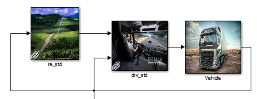
112. Theory on both the EMs and the ICE. An optimized ECMS would in principle minimize the use of the ICE, thus minimizing the fuel consumption. The propulsion or braking sub-model contains logic gates which, for instance, en- sures the vehicle is not using the engines to accelerate and brakes to decelerate at the same time. The sub-model also contains logic for the battery, ensuring it is not operating beyond physical limitations. For a more in depth explanation of the sub-model, see section 3.1.2. 2.3 Global Simulation Platform The Global Simulation Platform (GSP) is Volvo Group’s internal simulation soft- ware, used primarily as a tool to estimate the fuel consumption of heavy vehicles on any given operating cycle. The general structure, shown in figure 2.2, is very similar to VehProp. GSP con- sists of the same three sub-models as VehProp, i.e. environment (re_std), driver (drv_std), and vehicle (Vehicle) sub-models. Figure 2.2: General structure of Volvo Group’s Global Simulation Platform. The existing reinforcement learning controller [1] developed in GSP is fully enclosed within the vehicle sub-model, which means that the porting of required functionality from GSP to VehProp is a matter of fitting the right inputs to the RL agent. Since these inputs are quite general (i.e. speed, speed limit, slope etc.) this does not present a major challenge. 2.4 QSS Toolbox QSS Toolbox [16] is an open-source, light weight vehicle simulation platform devel- oped at ETH Zürich. The platform performs quasi state, backwards simulations of vehicles. This means the model calculates the necessary force on the vehicle, given a velocity at each time step. These forces are used to calculate all parameters of 12
2. Theory

the vehicle such as engine and brake power. The backwards simulation approach
eliminates the need for a driver to be simulated, such as a PID controller, because
the velocity for each time step is set before the simulation begins. This also means
that it is not possible to implement an RL agent to control any of the parameters
that would be controlled by the driver, for example controlling the brakes of the
vehicle. Furthermore, the backwards simulation approach generally requires less
computation time than the forward simulation approach.

QSS Toolbox is suitable for verification of data, if the velocity of a given cycle
is known. The backwards simulation approach ensures no differences in how the
vehicle is controlled between two different simulation platforms, since there is no
driver element in QSS Toolbox. As long as vehicle parameters are same, and the
vehicle is modeled correctly, a simulation done in QSS Toolbox should yield the
same results as a simulation done on another platform.

Running simulations in QSS Toolbox is fairly simple for one which is accustomed
to MathWorks Simulink, the platform is fairly small and mainly set up through
masks in the model. For further explanation and examples see [16], or if needed the
Mathworks Simulink documentation.

2.5     Reinforcement Learning Toolbox
The Reinforcement Learning Toolbox [17] from MathWorks is a library of functions
and blocks in Matlab/Simulink, enabling the training, implementation and verifi-
cation of reinforcement learning controllers in Matlab and Simulink environments.
Agent policies can be developed using several different methods and algorithms. The
toolbox supports import of existing policies, allowing for training of an RL agent in
alternative, open-source software libraries such as TensorFlow, Keras and PyTorch.

The RL toolbox is well-suited to this project due to the excellent integration with
Simulink environments, enabling easy experimentation with RL controllers in a va-
riety of vehicle models. A specific implementation of an RL controller, in this case
inside of main_withOC_hybrid_RAmod6.slx, can easily be carried over to other
vehicle models, if the overall structures and output variables are similar.

2.5.1    Agent block
The agent block in the Reinforcement Learning Toolbox is easily implemented in a
Simulink environment (see figure 2.3), taking in three input signals:

  • observation– the current state, on which the agent bases its action
  • reward– a scalar value based on any number of variables for the agent to
    maximize
  • isdone– a condition to tell the agent when to end a training episode in the
    context of the Simulink model (in this case when the operating cycle is com-
    pleted)

                                                                                  13
2. Theory Figure 2.3: Reinforcement learning agent block in Simulink. and outputting an action signal, defined in the setup of the agent. Properly implemented with a suitable reward function, this block may replace a traditional controller (e.g. PID controller). Rather than using a traditional feed- back loop calculating an action by looking at the error (i.e. the difference between the desired and actual state), the RL agent strives to maximize the reward provided by the reward function. (In this case the error is only one of the parameters in the reward function) 2.5.2 Creating agent environment The Simulink environment in which the agent acts is loaded with the use of the rlSimulinkEnv function, providing information about the Simulink model to be run and the location of the RL agent in it, as well as the properties of the input/output signals of the RL agent block. These include limits and dimensions of the signals, and the signal types, that is if the signals are continuous or discrete. The input signal, observation, is a continuous signal and is defined by the rlNu- mericSpec function, with no limits to signal size and a dimension that is equal to the size of the state vector. On the other hand, the output signal, action, is a dis- crete, scalar signal and is defined by the rlFiniteSetSpec function. The limits to the signal output depend on the application of the agent, and are defined by a vector containing all possible output signals. 2.5.3 Creating PPO agent The RL agent’s decision-making consists of an actor and a critic. The actor repre- sents the current policy and decides an action a to take given a state s. The critic represents the value function, determining the expected reward from following the policy π from the next time-step onwards, given a certain discount factor γ. In a PPO RL agent, both of these functions are approximated by neural networks, mak- ing use of the Deep Learning Toolbox. Setting up the PPO RL agent, there are several options to set for agent train- ing, in regards to both policy evaluation and policy adaptation: 14
2. Theory

  • Experience horizon– the number of time-steps the agent takes before adapt-
    ing its policy
  • ClipFactor– limits the change in the policy update (specific to the PPO
    algorithm, which limits the size of the policy change)
  • EntropyLossWeight– a higher value promotes the agent to explore, (more
    likly to not be stuck in local optima)
  • MiniBatchSize
  • NumEpoch
  • AdvantageEstimateMethod– method of estimating future advantages (GAE
    (Generalized Advantage Estimate) is used)
  • GAEFactor– smoothening factor for GAE
  • SampleTime– length of a timestep
  • DiscountFactor– used in policy evaluation to weigh future rewards against
    immediate reward of an action (the previously mentioned discount factor γ)

The neural networks that approximate the actor and critic are also customizable.
Both require information about observation and action dimensions and limits, pre-
viously defined in the agent environment as obsInfo and actInfo.

2.5.4    Training agent
A training session is started by using the train function. One training episode is
one execution of the Simulink model, running until the agent isdone criteria is met.
Alternatively, an episode can be completed once a certain number of time-steps have
been completed.

Once certain criteria are fulfilled, a session of training can be terminated. These
criteria can be in regards to the agent behavior (i.e. once a certain episode reward
or average reward is reached) or the session length (i.e. the number of training
episodes). If the result of the agent behavior is satisfactory, simulations can be run
with the trained agent using the sim function.

                                                                                   15
3
Methods
Description of the methods used to design a platform for reinforcement learning
research.
3.1 Implementation of an RL controller in Veh-
Prop using Reinforcement Learning Toolbox
3.1.1 RL agent block
The RL agent block continued previous work done by Chalmers students. [1]
Figure 3.1: Simulink block containing the RL agent.
The RL agent block, shown in figure 3.1, is designed to deliver the necessary inputs
to the RL agent as well as handling the output of the agent, i.e. the action. Among
the inputs are the four states of the RL application. These are written below in
vector format.
vt
v̄
t
S= .
v̄t+δt
αt
These include the current speed, vt , the current speed limit, v̄t , the speed limit a
fixed distance ahead, v̄t+δt (set to 250 meters ahead), and the slope of the road, αt .
The two other inputs to the RL block are the current position, position and current
service brake usage, sbrake. These inputs are not used in the observation vector
since they are not to be used in a policy evaluating whether or not to brake in a
particular state, but they must be implemented in the reward function to ensure
that the deployed policy exhibits the desired behavior. For instance, the trained
163. Methods
policy is of no use if it makes the truck stand still (position not increasing), and it is
not satisfactory if it does not minimize the service brake usage sbrake. The current
position is also used to check if the simulation cycle is done, and if so sends a signal
isdone to the RL agent, ending the training cycle or simulation run.
There is only one output from the RL block which is the action taken by the agent.
The action is an electric motor brake demand, the signal is discrete and is separated
into 11 discrete steps which range evenly from 0 to 100% of the maximum electric
motor brake capacity.
3.1.2 Driver/RL agent interaction
Early on, complex problems were encountered when implementing the RL controller
in the vehicle model. Even when the problem is delimited to only taking braking
action with the RL controller, one must carefully consider the interaction between
the driver and the RL agent. Since the vehicle model is a hybrid electric vehicle
(PHEV), deceleration demands can be met through the use of service brakes or by
recuperating energy to the battery through the electric motors (EMs). Similarly to
the propulsion case, one must decide how to split the load, altough this is rather
straight-forward without the RL agent since the braking energy is lost in the form
of heat when using the service brakes; thus the EMs should be used to the greatest
extent, up to their maximum capacity (physically limited by speed, SOC, etc.).
The RL agent is located in the PropulsionorBraking block in VehProp, depicted in
figure 3.2. As the name suggests, this block recieves multiple signals containing the
driver’s power demand– general need for acceleration/deceleration in the form of
powerDemandPwt and specific demands on the electric/combustion engines in the
form of powerDemandBatt and powerDemandEngine (calculated by ECMS)– and
outputs signals detailing power output from the service brakes, the electric motors
and the combustion engine. Note that the power output from the electric motor can
assume both positive and negative values, depending on the driver’s action and the
split between electric/combustion propulsion or service brake usage.
The current implementation of the RL agent allows the agent to completely override
the driver’s actions at any time. Rather than powerDemandPwt acting as a condi-
tion for switches, the RL agent’s action controls all power outputs, deactivating the
combustion engine and providing a negative, braking, power output to the electric
motors when braking action is taken by the RL agent. This eliminates the risk of
the driver accelerating when the RL agent is braking, and allows the RL agent to
exploit its knowledge gained over a training cycle.
Originally, there was some level of collaboration between the driver and the RL
agent– when the driver demanded a greater braking output than the RL agent pro-
vided (if any at all). This initially posed a challenge from a modeling perspective,
requiring a way to determine service brake power output given two conflicting power
demands. In order to maintain a certain level of control for the driver, the calcu-
173. Methods Figure 3.2: PropulsionorBraking block in Simulink. lation of the service brake power output was designed in order to fully cover the braking need of the driver, which meant using the service brakes to cover the differ- ence between the driver’s need and the output of the RL agent. After some revision, the implementation of the RL agent was changed in order to ensure causality between the agent’s actions and the ensuing reward, the reasoning being that the reinforcement learning loop would be broken by the driver’s actions. In the case where the driver demanded braking action while the RL agent took no action, the result would be usage of the service brake, causing a change in the environment attributable to braking, despite no action being taken by the RL agent. Instead, the RL agent was given full control of braking action and the input of the driver was limited to acceleration, thereby decreasing the complexity of the PropulsionorBraking block and allowing the RL agent to act, unhindered by the actions of other agents in the environment. 3.2 Verification of VehProp The purpose of QSS Toolbox in this project is to provide verification of VehProp. If a simulation is run in VehProp the velocity for each time step can be saved and used as input to the backwards simulation in QSS Toolbox. Data from both simulations can then be compared to assess the accuracy and plausibility of VehProp. A simple flow chart of the process can be viewed in figure 3.3. Similar comparisons between backwards and forward simulation have been done. 18
3. Methods

                    vehprop simulation:

                      Fuel%flow           Engine%map       Acceleration     Speed

                                               Export/Import

                    QSS-toolbox-simulation:

                      Speed         Acceleration          Engine%map      Fuel%flow

Figure 3.3: Flow chart of simulation verification.

One paper [18] shows that the total energy consumption of a power propulsion
system can be comparable in absolute measures. However, problems with the non-
controllable backwards simulation can arise when a reference speed is set, specifically
with the maximum power output of the propulsion system. This is due to the lack
of control within the simulation. However, this should not be a problem in the
case of this project, since the forward simulation in VehProp is controlled and so
the acceleration requirements of the speed changes can not exceed the maximum
acceleration limit of the vehicle.

3.3      RL agent setup
Once the RL block is implemented in the model, it can no longer be run directly
from the Simulink model without prior training. Instead, it has the option to be
run in training mode, or in simulation mode, where the trained agent is deployed.
The setup file is divided into three sections, setup of the environment, options for
the agent (algorithm), and options for the training.

3.3.1     Agent options
The main source of information regarding PPO algorithm parameters in the Rein-
forcement Learning Toolbox is the MathWorks documentation [19], the used options
are shown in table 3.1.

                                                                                              19
3. Methods
Table 3.1: The parameters used in the agent options.
Parameter Value
Experience horizon 512
ClipFactor 0.2
EntropyLossWeight 0.02
MiniBatchSize 64
NumEpoch 3
AdvantageEstimateMethod ’gae’
GAEFactor 0.95
SampleTime 1
DiscountFactor 0.9995
The optimal parameters were determined by trial and error. The aim is for the agent
to explore during training but at the same time to converge within a reasonable
number of time (no more than 2000 training episodes), in order to allow for training
of the agent on any personal computer.
3.3.2 Training options
The StopTrainingCriteria option terminates the training session when the maximum
numbers of training episodes have been completed, in this case we set the training
session to terminate upon completing 2000 training episodes. The MaxStepsPerEpisode
option is the number of time steps the agent is allowed to train in an episode before
starting a new episode. We set this to 1000, which means the distance the agent trav-
els varies from episode to episode. Alternatively, the previously mentioned isdone
criteria can be used to set a fixed distance traveled that terminates the episode.
3.3.3 Training process
During training, 50-200 episodes are usually sufficient to see some level of conver-
gence, which allows for experimentation in the reward function and the RL Toolbox
options. A training session can be run in about 10 minutes on a laptop. The agent
is not training on the whole cycle since it would require too much processing power.
Instead, the agent is trained on a shorter distance, more precise 1000 time steps.
Since each training episode is fixed to 1000 time steps, the total distance travelled
will vary from episode to episode depending on the agent’s actions. Even though the
distance varies, it usually covers roughly 10 km in each episode. This is deemed to
be sufficient to allow the agent to learn the behaviors that are necessary to perform
well on the whole cycle.
The training was usually combined with debugging and verification of the agent,
including scoping of the vehicle speed and braking in Simulink, and making changes
thereafter. By comparing the converged agent to an earlier training episode, we
could distinguish the way in which the agent adapted. Eventually, the agent was
203. Methods trained for a large number of episodes, the agent was trained for 2000 episodes which took about 3 hours on a laptop. 3.4 Reward function The reward function is a MATLAB script that takes in any number of input signals and produces a single scalar output, and since the VehProp model can provide any signal of interest in the truck, there are many different combinations of inputs to the reward function one could choose. Since calculating the value of a scalar function is not computationally heavy, changes can be made in the reward function without adding to the training/simulation time, allowing for rapid experimentation. The RL agent has two stated goals: to follow the reference speed (speed limit) as closely as possible while minimizing fuel consumption, in this case by maximizing the proportion of braking done by EM. In order for the agent to learn how to achieve these goals, the reward function must be defined as a scalar function that grows as performance improves, so the reward function should increase as the speed error decreases and as the service brake usage decreases. The only input signals to the reward function deemed necessary are the speed and speed limit from the state vec- tor as well as the service brake usage. The chosen reward function is as follows: % obs 1 = current velocity % obs 2 = current vlim % sbrake = Service brake demand error=obs(1)-obs(2); reward=3.5+2*sbrake*1e-6-error^2*1e-3+exp(-0.25*error^2) The input signals are scaled down to the same order of magnitude to properly bal- ance the two and keep the size of the total reward on a manageable level, and a small number (3.5) is added to keep the total reward positive. In order to discourage the RL agent from maintaining a speed error and braking with the service brakes, a punishment is introduced in the reward function. The punishment grows quadrat- ically with the speed error and linearly with the service brake usage, encouraging the RL agent to keep the truck in the cruising zone. The sbrake signal is negative, explaining the positive sign in the reward function. Additionally, a large reward for maintaining a small speed error (
3. Methods

                                                                                                          2
                                                       3.5-2*sbrake*10 -6 -error 2*10 -3 +e -0.25*error
                                                                                                                                4.5

                                  20
                                                                                                                                4

                                  10
                                                                                                                                3.5

                                    0                                                                                           3
             Speed error [km/h]

                                                                                                                                2.5

                                                                                                                                      Reward
                                  -10

                                                                                                                                2
                                  -20

                                                                                                                                1.5

                                  -30
                                                                                                                                1

                                  -40
                                                                                                                                0.5

                                  -50
                                        0   50   100       150      200      250      300      350            400   450   500
                                                                 Service brake usage [kW]

Figure 3.4: Reward function plotted against speed error and service brake usage.

means there is a risk of the reward function being gamed by the agent extending
the training episode for as long as possible. In this case, each training episode is set
to a fixed number of time-steps (1000) in order to avoid this risk.

3.5      Improving ECMS in VehProp
The ECMS implemented in VehProp is not optimal, it does not keep the SOC around
the desired level in a stable way. A stable SOC is desirable to be enable the use of
EMs and EM brakes at any time, which is not possible if the SOC is either too high
or too low. By enabling the use of the EMs at will by the driver, the use is expected
to increase. This will in turn decrease the overall fuel consumption of the vehicle.

In figure 3.5 the SOC and equivalence factor is shown, attempts are made to stabi-
lize the equivalence factor and in turn stabilize the SOC. The attempts are made by
systematic trial and error, since the effects are easy to verify in figures such as 3.5.
The total fuel consumption of the cycle, the average speed of the vehicle as well as
the change of SOC are also a part of the data needed to verify the changes made to
the ECMS.

22
3. Methods
SOC and EqFactor
2
SOC
EQFactor
1.8 SOC Reference
1.6
1.4
1.2
1
0.8
0.6
0.4
0.2
0
0 20 40 60 80 100 120 140 160
Distance [km]
Figure 3.5: SOC and equivalence factor plotted over distance.
234
Results
In this chapter the results of the trained RL agent, as well as the improvements to
VehProp, are presented.
4.1 Agent convergence
The training of the agent provides information about the reward in each training
episode, the average episode reward for the whole training session, and the episode
Q0 , i.e. the estimate of the long-term discounted reward. The result of the agent
training session is illustrated in figure 4.1.
Figure 4.1: Episode rewards in the final agent training session.
After 600 training episodes, the episode reward converges to roughly 364. Minor
fluctuations (4. Results
performs sub-optimally and yields a low episode reward. After another 100 episodes,
the reward returns to the previous level around 364, maintaining a high reward for
a few hundred episodes and dropping again. This pattern is repeated in the whole
training session of 2000 training episodes.
It appears that the agent is stuck in a local optima at an episode reward of 364,
where it is unable to learn how to improve upon itself. Upon exploring further,
the policy worsens, yielding a low reward and the agent eventually returns to the
previous local optima. A plausible explanation for this behavior is that exploration
and exploitation are not properly balanced in the RL algorithm. Since the agent
learns from its own actions in the environment, it can be difficult to learn the desired
behavior of the designer if it is far away from the current behavior, without guidance.
The discount factor, clip factor and several other options in the RL algorithm are set
by the designer and these parameters inherently affect the agent’s learning process.
4.2 Vehicle speed
An important aspect of the agent’s behavior is the ability to follow the speed limit.
Therefore, the reward function is designed to punish the agent when the vehicle
deviates from the speed limit. However, the trained agent is not able to perform
well in this aspect, as shown in figure 4.2. The agent is unable to follow the speed
limit sensibly.
Actual speed and speed Limit Actual speed and speed Limit
35 35
30 30
25 25
vehicle speed [m/s]
vehicle speed [m/s]
20 20
15 15
10 10
Speed Limit
Actual speed
5 5
Speed Limit
Actual speed
0 0
0 20 40 60 80 100 120 140 160 0 5 10 15 20
position [km] position [km]
(a) Full cycle. (b) Training cycle.
Figure 4.2: Speed and speed limit plotted over the the route.
Despite being punished for deviating from the speed limit, the agent frequently does
so, which could be a consequence of the punishment being too low. On the other
hand, the agent does not deviate as much from the speed limit on the training cycle,
so it is possible that the sample size of the training cycle is too small for the agent
to learn when to brake in a general sense. However, the agent still exceeds the speed
limit on the training cycle by up to 10 m/s, which is not acceptable. Ideally, the
254. Results
agent should not converge to a solution with this behavior.
The large drops in speed compared to the speed limit depicted in figure 4.2 are not
unique to the RL agent. The same drops are found when the standard driver model
of VehProp is used for braking, as shown in figure 4.3. These drops are a result of a
positive road grade, i.e. the vehicle is moving uphill. As the drops in speed happens
at the same time for the RL implementation as it does for the driver controller, the
drops in speed are not entirely at fault of the agent. This leads to the conclusion
that the agent is responsible for the surges in speed but not the drops.
Actual speed and speed Limit
35
Speed Limit
Actual Speed
30
25
vehicle speed [m/s]
20
15
10
5
0
0 20 40 60 80 100 120 140 160
position [km]
Figure 4.3: Speed and speed limit without RL implementation.
Analyzing the data from simulation shows that the agent has converged to a solution
which is not taking any action to brake. This causes the agent to perform well in
upward slopes since braking is usually not necessary in those states, but worse in
downward slopes. The correlation between speed and road grade is depicted in figure
4.4, as well as the non-braking action in figure 4.5. The absence of negative power
output from the batteries means no regenerative braking is performed. One of the
states in the current implementation is road grade, so the agent should be able to
detect changes in angularity of the road. This should be an advantage for the agent,
as the agent has the option to brake before the downhill slope. This should result
in reduced use of service brakes and greater chance of following speed limit, but the
agent does not display this behavior.
26You can also read