VOLATILITY SPILLOVER AND DYNAMIC CORRELATION BETWEEN THE CARBON MARKET AND ENERGY MARKETS
←
→
Page content transcription
If your browser does not render page correctly, please read the page content below
Journal of Business Economics and Management
                                                                                           ISSN 1611-1699 / eISSN 2029-4433
                                                                                            2019 Volume 20 Issue 5: 979–999
                                                                                   https://doi.org/10.3846/jbem.2019.10762

       VOLATILITY SPILLOVER AND DYNAMIC CORRELATION
      BETWEEN THE CARBON MARKET AND ENERGY MARKETS

                   Yufeng CHEN1, 2, 3*, Fang QU1, Wenqi LI1, Minghui CHEN4
                   1School
                         of Economics, Zhejiang Gongshang University, Hangzhou, China
   2College of Business Administration, Capital University of Economics and Business, Beijing, China
        3Center for Studies of Modern Business, Zhejiang Gongshang University, Hangzhou, China
                     4MBA School, Zhejiang Gongshang University, Hangzhou, China

                                   Received 21 December 2018; accepted 18 June 2019

      Abstract. This paper studies the volatility spillover and dynamic correlation between EU emission
      allowance (EUA) prices and energy prices by considering three energy commodities, including oil,
      gas, and coal. The asymmetric BEKK model is employed for multi-phase analysis of EU ETS, yet
      only a little empirical evidence backing up the existence of volatility spillover between EU ETS and
      energy markets, i.e., the establishments of the EU ETS may not effectively restrict and influence
      energy markets. The time-varying conditional correlation between EUA and each of energy prices
      is analyzed. The dynamic correlation shows there is a relatively stable, positive correlation between
      the EUA and Brent oil, natural gas. However, modeling the dynamics correlation also suggests that
      the correlation between the EUA and the natural gas, coal became weaker and more volatile since
      second and third phases, especially after the Global Financial Crisis in 2008, which may indicate
      that the demand reduction in emission allowances caused by the economic slowdown far exceeds
      the reduction in the annual restraint of EU ETS.

      Keywords: volatility spillover, EU ETS, EUA, energy price, asymmetric BEKK model, dynamic
      correlation.

      JEL Classification: C32, G12, Q43.

Introduction
Volatility means risk, and volatility spillover represents risk transfer between diverse finan-
cial markets. Understanding the volatility spillover between EU ETS and energy market in
various phases has vital reference significance for the establishment and improvement of
emission trading schemes in countries around the world. Carbon emission allowance is one
of the most essential commodities in the carbon market that is recognized as an efficient way
to answer the greenhouse gas (GHG) emission problem. It has been traded on exchanges and
Over-The-Counter (OTC) market since the announcement of Kyoto Protocol. The European

*Corresponding author. E-mail: chenyufeng@gmail.com

Copyright © 2019 The Author(s). Published by VGTU Press
This is an Open Access article distributed under the terms of the Creative Commons Attribution License (http://creativecommons.
org/licenses/by/4.0/), which permits unrestricted use, distribution, and reproduction in any medium, provided the original author
and source are credited.
980 Y. Chen et al. Volatility spillover and dynamic correlation between the carbon market and energy...
Union Emission Trading Scheme (EU ETS) was the first one in the world that was established
in 2005 and it is now still the world’s largest emission trading scheme, which covers sectors
that account for approximately 45% of Europe’s total GHG emissions, and it is the most rep-
resentative emission trading scheme in the world (Hu, Crijns-Graus, Long, & Gilbert, 2015).
As of 2017, there are 21 operating emissions trading schemes in the world, and economies
with an ETS in place produce more than 50% of global GDP and are home to almost a third
of the global population. More countries, including China, United States, Mexico and Bra-
zil start to develop their own emissions trading schemes, which makes the carbon market
become one of the most promising markets for investors. Thus, it is necessary and vital for
policymakers, regulated energy enterprises and investors to understand the fundamentals of
the carbon price and the factors that affect it. Moreover, as more financial corporations and
investors are investing the derivatives of the emission allowance, it is useful for them to fully
understand the change of volatility behind the prices.
The energy price is one of the important factors since the amount of CO2 emission is
associated with what kinds of energy used. The use of crude oil, natural gas, and coal is the
main source of CO2 emissions (Fan, Jia, Wang, & Xu, 2017), and the impact of such energy
price on carbon price is extremely significant. Although these commodities may come from
different financial markets, their attribute is the same, reflecting the real price of such energy.
Specifically, the sharp and sustained increase of energy price and the inelastic demand for
energy will induce large demand for emission allowance and hence a higher carbon price.
Furthermore, this paper is interested in how the carbon prices response to shocks on the en-
ergy prices, which is significant for risk management and portfolio optimization. Mansanet-
Bataller, Pardo, and Valor (2007), Alberola, Chevallier, and Chèze (2008a, 2008b), Keppler
and Mansanet-Bataller (2010) found empirical evidences showing the prices of energy, elec-
tricity and factors like weather and markets’ expectation are the leading factors that affect the
carbon prices. Recent research has focused on the impact of EU ETS on energy conservation
and emission reduction in the aviation sector and energy efficiency management (Cui et al.,
2017; Nava, Meleo, Cassetta, & Morelli, 2018). This is because after January 2012, the aviation
sector was forced to be included in the EU ETS and the transportation sector has become a
typical purchaser of EU ETS, which they mainly use oil and coal.
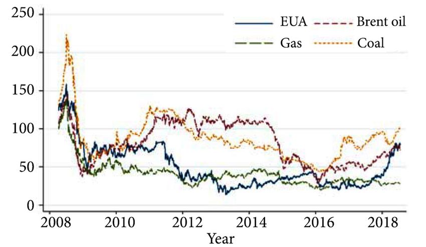
Figure 1. Daily prices of the EUA and the energyJournal of Business Economics and Management, 2019, 20(5): 979–999 981
Meanwhile, after the Global Financial Crisis, a potential fact can be observed from the
Figure 1, the oil and the coal prices seem to have a negative trend against the EU emission
allowance (EUA) price, and this trend is especially significant during the year 2014 to 2016.
From the perspective of financial markets, the emission allowance and energy are alterna-
tive investments. In other words, when energy prices rise, energy consumption will declines,
which lead to a trend of decline in CO2 emissions, may eventually lead to a fall in the car-
bon price of the EU ETS. This economic intuition motivates us to reevaluate the correlation
between the carbon and energy prices. The volatility spillover is a measure of how much a
shock in the price volatility of a financial asset will affect another asset’s price. It can also be
interpreted as a proxy for information transmitted between two markets and has been widely
used in the application and researches of economics and finance (Hamao, Masulis, & Ng,
1990; Baele, 2005; Du, Yu, & Hayes, 2011). Moreover, multivariate GARCH models have of-
ten been used in previous literature to study the volatility spillover of the energy and carbon
markets, and the most representative methods are the BEKK model and the DCC model.
Efimova and Serletis (2014) use the data from the energy market to show that the multivari-
ate GARCH model performs well in studying the correlation and spillover effects. Zhang and
Sun (2016) explore the volatility spillover between the EU ETS and the fossil energy market
using a threshold DCC. Dhamija, Yadav, and Jain (2016) study the volatility of EU ETS and
energy prices, and they found that the asymmetric GARCH model is relatively optimal.
Currently, the EU ETS is divided into four phases (phase I: 2005–2007, phase II: 2008–
2012, phase III: 2013–2020), and the fourth phase (2021–2030) has not yet arrived. Thus, this
research focuses on the situation of the EU ETS in the I to III Phases so far. EU ETS works on
the “cap-and-trade” principle, i.e., the companies’ emission is subject to the cap set annually
and they receive, buy and sell emission allowances within the scheme. Consequently, the total
amount of carbon emissions of the EU ETS remains constant during a trading cycle. The cap
of carbon emission is reduced over time so that total emissions fall. So far, EU ETS covers
around 45% of total GHG from 31 countries (all 28 EU countries plus Iceland, Liechtenstein
and Norway) and the emission of CO2 from power plants, a wide range of energy-intensive
industry sectors and transportation sector. Since its commencement, a number of researches
have begun to discuss the allocation process and the mechanism of the EU ETS (Ellerman,
2008; Ellerman, Convery, & De Perthuis, 2010; Parsons, Ellerman, & Feilhauer, 2009; Hu,
Crijns-Graus, Long, & Gilbert, 2015; Dhamija, Yadav, & Jain, 2016; Jiménez-Rodríguez, 2019)
and most studies takes EUA price as the carbon price.
To sum up, compared with the previous literature, the potential contributions of this ar-
ticle are concentrated in the following aspects: Firstly, this paper discusses the correlation and
volatility spillover of EU ETS to the energy market on multi-phase perspective. Because of
the different operating time of the EU ETS, the economic conditions and trading rules faced
by this scheme (EU ETS) in different periods are also diverse. Since many literatures have
used the entire cycle or a certain phase of the EU ETS as a research sample (Alberola, Cheval-
lier, & Chèze, 2008a, 2008b; Chevallier, 2011; Eugenia Sanin, Violante, & Mansanet-Bataller,
2015; Dhamija, Yadav, & Jain, 2016; Zhang & Sun, 2016; Wang & Guo, 2018), supplement-
ing multi-phase research has practical significance. Secondly, the asymmetric BEKK model
is a powerful weapon for the study of volatility spillovers. This model not only measures the982 Y. Chen et al. Volatility spillover and dynamic correlation between the carbon market and energy...
direction of volatility spillovers, but also can observe the magnitude of volatility. On this
basis, this paper considers dynamic correlation and further investigates the fluctuations in
the relationship between EU ETS and energy markets from the time-varying perspective.
Finally, this paper also examine the asymmetry of the volatility spillover effects between the
EU ETS and the energy markets in various phases, which present explanation the impact of
economic events on spillover.
The structure of this paper is organized as follows: Section 1 presents the literature review.
The data and the models employed are described in section 2 and section 3. In section 4,
this paper provides the empirical results and analysis. The section 5 is a discussion of details.
Conclusions, policy implications and the further research are shown by final section.
1. Literature review
It is widely accepted that the CO2 emission allowance price is related to energy prices, tem-
perature condition and power prices (Mansanet-Bataller, Pardo, & Valor, 2007; Keppler &
Mansanet-Bataller, 2010; Chevallier, 2011; Aatola, Ollikainen, & Toppinen, 2013; Eugenia
Sanin, Violante, & Mansanet-Bataller, 2015; Kanamura, 2016; Lin & Jia, 2017; Fan, Jia, Wang,
& Xu, 2017; Soliman & Nasir, 2018; Dutta, Bouri, & Noor, 2018). Mansanet-Bataller, Pardo,
and Valor (2007) used daily data in the OLS regression and found daily CO2 emission price
change was related to the price changes of crude oil, natural gas and extremely hot and cold
temperature in German. Alberola, Chevallier, and Chèze (2008a) used daily spot data and
extended the previous literature by considering structural breaks, finding the energy funda-
mentals and extremely cold temperature does have impacts on the price changes. Different
from the previous findings, Aatola, Ollikainen, and Toppinen (2013) built an equilibrium
model of the emission trading market and tested it with daily forward data using OLS, IV
and VAR models. Their results show there is a clear and stable correlation between the fun-
damentals and the price of EUA. Except for energy, temperature and power prices, Alberola,
Chevallier, and Chèze (2008b) first showed three industries’ production (combustion, paper,
and iron) has a large impact on EUA price changes using linear regression and TGARCH
model. Using a supply and demand based correlation model, Kanamura (2016) report a
positive energy price impact on EUA prices. Ibrahim and Kalaitzoglou (2016) proposed an
asymmetric information microstructural pricing model in which price responses to infor-
mation and liquidity vary with every transaction and find that expected trading intensity to
simultaneously increase the information component and decrease the liquidity component
of price changes.
Some of researches have started to characterize EUA price volatility that is meaningful in
the financial application such as risk management and carbon pricing. Benz and Trück (2009)
found that regime-switching or GARCH model are the best to capture the dynamic behavior
and volatility of EUA returns, which is very helpful for risk management and cost control.
Chevallier (2011) extended that Benz and Trück’s (2009) by taking other fundamental driv-
ers of the carbon price into account and found the economic activity is a key determinant
of the carbon price returns. Lutz, Pigorsch, and Rotfuß (2013) analyzed the nonlinearity
correlation between EUA price and its fundamentals by considering regime-switching intoJournal of Business Economics and Management, 2019, 20(5): 979–999 983
a GARCH type model and characterizing their time-varying influence. Conrad, Rittler, and
Rotfuß (2012) chose high-frequency data and applied a fractional integrated asymmetric
power GARCH model to show conditional heteroscedasticity and long memory property of
EUA returns, which is crucial in financial practice. Xu, Deng, and Thomas (2016) investigate
the impact of financial options on reducing carbon permit price volatility under a cap-and-
trade system and report that introducing financial options in a banking environment of-
fers more flexibility to risk management in carbon permit trading. Campiglio (2016) argues
carbon pricing in itself may not be sufficient and discusses the potential role of monetary
policies and macroprudential financial regulation.
Many studies used the exchange rate in financial markets as the research object to explore
its volatility and spillover effects (Akar, 2017; Bubák, Kocenda, & Zikes, 2011; Hong, 2001).
The employ of high-frequency data and spillover index is also the mainstream scheme on
research of volatility (Chen, Li, & Qu, 2019). These studies have played a pioneering role
in applying volatility to the discussion of carbon trading schemes. However, as the interac-
tion among different financial markets is unsteady, forecasting volatility should take other
variables into consideration. A few pieces of research have discussed mutual interaction and
volatility spillover between EUA market and fundamentals. Fezzi and Bunn (2009) used a
structural and co-integrated vector error-correction model (VECM) to consider the pos-
sible mutual interaction between gas, carbon, and power which first provide a framework
that included both long-run equilibrium and short-term effects. Reboredo (2014) proposed
a MCARR model to capture this effect between oil market and EUA market using daily
prices of EUA future and found no spillover between them. Mansanet-Bataller and Soriano
(2009) applied BEKK model proposed by Engle and Kroner (1995) to characterize the vola-
tility transmission among oil natural gas and EUA market. In contrast to Reboredo (2014),
Mansanet-Bataller and Soriano (2009) found bidirectional volatility transmission between
oil and EUA price and the natural gas market has unidirectional volatility transmission to
the other markets. Wang and Guo (2018) employ the spillover index constructed by Diebold
and Yilmaz (2009, 2012) to investigate the asymmetric volatility spillover effect between the
carbon market and three energy prices including WTI oil, Brent oil and EU natural gas. Ji,
Zhang, and Geng (2018) considers the correlation between electricity prices and the carbon
market and believe the electricity prices to be the mainly recipient of information transfer.
Overall, most studies have considered significant volatility spillover effects between the EUA
market and other financial markets.
It can be found that carbon emissions as a special financial commodity, most of the
previous research from the financial point of view, using time series analysis method (VAR,
VECM, GARCH type, BEKK and so on) to discuss the correlation and mean or volatility
spillover effect between carbon market and energy markets. Regrettably, few studies have
focused on coal market because the proportion of coal in primary energy consumption in
Europe has already fallen dramatically. But for developing countries such as China, Brazil and
India, the proportion of coal in primary energy consumption is still high, and considering
coal is an important reference value for these countries. Therefore, this paper extends the
previous studies by taking coal price and discussing the dynamic volatility spillover between
the traditional energy markets and EUA market.984 Y. Chen et al. Volatility spillover and dynamic correlation between the carbon market and energy...
2. Data
The EUA daily future price from the European Climate Exchange (ECX) is used as the carbon
price. For the oil, coal and gas price, the price of the Brent future contract and the Rotterdam
Coal future price from the International Petroleum Exchange (IPE), and the price of gas
future contracts from NYMEX, were selected as research samples. All data series have been
collected from WIND Information Financial database.
As shown in the Figure 2, in the phase I of the EU ETS, the price of EUA future followed
two major slowdowns. One occurred in April 2006 because the announcement of verified
emission amount implied an over-allocation of EUA. The other slump, at the end of the
phase I, resulted from not only over-allocation but also the banking restriction, leading to
selling-off and price collapse (Parsons, Ellerman, & Feilhauer, 2009; Zhang & Wei, 2010). The
variance of EUA returns was very large after December 17, 2007 because of the adjustment
by authority, so this paper decides to discard the data after that date to get a stationary series.
In addition, because of the availability of the coal data, this paper analyze the existence
of spillover between EUA with oil and EUA with natural gas and their dynamic correlation
during the phase I, and the data from April 22, 2005 to December 17, 2007. For the analysis
of the II and the III phase, the sample data is from April 08, 2008 to December 31, 2012 that
covers almost all second period of the EU ETS and January 2, 2013 to July 17, 2018 that is the
phase III so far. All price series are converted into euro using exchange rates from European
Central Bank in order to remove the effect of exchange rate variability. Therefore, the data
period and the number of observations are shown in Table 1. The log returns are calculated as
follows: =rt 100 × ln ( Pt Pt −1 ) . P uses the settle price for all series. These data periods contain
several important periods in which the energy markets experienced a large instability, for
example, Global Financial Crisis in 2008 and oil price slowdown in 2015.
Figure 3 and 4 display the returns of the EUA, Brent oil, natural gas and coal from phase
II and phase III. All returns series show volatility clustering. Table 2 presents the summary
statistics of all the log returns of EUA and energy in three phases of the EU ETS. The aug-
mented stationarity test (ADF, PP and KPSS) shows all series are stationary. The similar mean
value is displayed, but differs in the standard deviation of series from phase to phase. The
log returns of EUA have the largest standard deviation in the first and the third phase, while
the log returns of natural gas have the largest standard deviation in the second phase. The
Figure 2. Daily EUA Price from the phase I of EU ETSJournal of Business Economics and Management, 2019, 20(5): 979–999 985
skewness, kurtosis as well as Jarque-Bera test show that only the log returns of Brent in the
first phase follow the normal distribution. The log returns of EUA have large kurtosis and
Jarque-Bera statistic in the first phase, which results from large instability. The Ljung-Box test
of the four series has different results from each other. Even the same series have inconsistent
test results in different phases. The Q statistic shows that the log returns of EUA are autocor-
related in the first to third phase. The coal and natural gas returns are autocorrelated only in
the second. This may be due to the grouping of samples, and it does not indicate that these
series do not have autocorrelation in the long run.
Table 1. Phase of EU ETS and the Number of Observation
Phases Start End Number of Observation
Phase I 2005.04.22 2007.12.17 661
Phase II 2008.04.08 2012.12.31 1180
Phase III 2013.01.02 2018.07.17 1383
Figure 3. Daily Log Returns of EUA and the Energy Futures from the phase II of EU ETS
Figure 4. Daily Log Returns of EUA and the Energy Futures from the phase III of EU ETS986 Y. Chen et al. Volatility spillover and dynamic correlation between the carbon market and energy...
Table 2. Descriptive Statistics for the Daily Log Returns of the EUA and the Energy Futures
Phase I Brent gas EUA
Mean 0.06 –0.02 –1.12
Std. dev 1.74 3.70 10.84
Skewness –0 .09 0.69 –3.11
Kurtosis 3.16 7.58 74.90
J-B test 1.61 633.39*** 143899.83***
ADF test –28.467*** –25.351*** –26.727***
PP test –28.479*** –25.368*** –26.742***
KPSS 0.09 0.09 0.09
Q(5) 14.12** 1.06 15.557***
Q(10) 15.63** 2.18 31.150***
Observation 661 661 661
Phase II Brent gas coal EUA
Mean 0.02 –0.06 –0.02 –0.10
Std. dev 2.27 3.48 2.01 2.74
Skewness –0.20 1.04 –0.88 0.13
Kurtosis 6.63 8.32 27.28 6.91
J-B test 663.25*** 1615.66*** 30945.47*** 759.58***
ADF test –36.75*** –38.74*** –32.95*** –8.73***
PP test –36.82*** –38.76*** –33.01*** –32.41***
KPSS 0.14 0.06 0.18 0.06
Q(5) 10.46* 26.20*** 22.19*** 10.68*
Q(10) 21.11** 40.21*** 46.77*** 20.75**
Observation 1180 1180 1180 1180
Phase III Brent gas coal EUA
Mean –0.03 –0.01 0.01 0.07
Std. dev 2.05 1.97 1.23 3.52
Skewness 0.09 –0.06 1.70 –1.35
Kurtosis 6.82 5.32 43.22 24.06
J-B test 843.99*** 311.28*** 93817.01*** 25968.64***
ADF test –40.560*** –38.249*** –36.470*** –38.098***
PP test –40.444*** –38.261*** –36.520*** –38.186***
KPSS 0.31 0.07 0.35 0.23
Q(5) 17.04*** 2.14 4.86 48.23***
Q(10) 18.31** 7.50 13.69 67.10***
Observation 1383 1383 1383 1383
*, ** and *** represent the statistics are significant in the confidence level of 10%, 5% and 1%.Journal of Business Economics and Management, 2019, 20(5): 979–999 987
3. Methodology
Based on the BEKK model proposed by Engle and Kroner (1995), which is not only to mea-
sures the direction of volatility spillovers, but it also can observe the magnitude of volatility
spillover. In addition, in order to investigate the asymmetry of volatility spillover, this paper
further employ the asymmetric BEKK mothed to analyze the spillover effect between the EU
ETS and energy market, which can explore to what type of news (good or bad) the volatility
spillovers between EU ETS and energy markets in different phases is more sensitive.
Let rt denote the asset’s returns, the typical BEKK model can be shown as follows:
rt = µ + et ; (1)
et | It −1 std ( 0, H t ) ; (2)
p q
( )
C0C0T + ∑ Ai et −i etT−i AiT + ∑ B j H t − j BTj ,
Ht = (3)
=i 1 =j 1
Where µ is a vector of constant of mean value. et is a vector of residual terms, which is
the source of volatility and risk. It −1 is the information set generated by the past values et .
Where Ai and B j are unrestricted k × k parameter matrices with C0 triangular. Assum-
ing that the et follows the normal distribution in conditional of the past information. The
conditional variance H t follows a BEKK model. It is easy to show that H t is guaranteed to
be symmetric and positive semi-definite in the above formulation because C0C0T is positive
definite. Eq. (1) to (3), the Eq. (1) is called the mean equation. For series with autocorrelation,
Eq. (1) is assumed to be a vector autoregressive (VAR) structure as follows:
p
ri ,t =αi + ∑ Ωk ri ,t −k + ei ,t . (4)
k =1
Where α is the k dimensional constant, Ω is the k × k parameter matrix, and et should
satisfy independent and identical distribution (i.i.d), consistent with Eq. (2). The Eq. (3) is
called the variance equation, and the et in Eq. (2) is used to create Eq. (3). Besides, the
BEKK model requires estimation of ( p + q)k ^ 2 + k(k + 1) / 2 parameters as the increase of
the number of k, p and q. The p and q are representing the level of the ARCH effect and the
GARCH effect. In order to avoid the problem of dimensional curse on BEKK model, this pa-
per consider the typical BEKK model with p= q= 1 . In order to further consider the asym-
metry of volatility spillover, connected with the concept of GJR-GARCH model (Glosten,
Jagannathan, & Runkle, 1993; Zhang & Sun, 2016), the following asymmetric BEKK(1,1)
model is employed:
Ht = ( ) ( )
C0C0T + A1 et −1eTt −1 A1 + B1H t −1 B1T + D1 zt −1ztT−1 D1 . (5)
The form of the D matrix is the same as the A and B matrices, and zt −1 is a k dimen-
sional column vector. When et – 1 is negative (et – 1 ≤ 1 it means bad news or negative shock),
the zt −1 = et – 1, else, zt – 1 = 0. Consequently, the matrix D measures the asymmetric effects
between the EU ETS and the energy markets. Moreover, many studies believe that there are988 Y. Chen et al. Volatility spillover and dynamic correlation between the carbon market and energy...
fat tails facts in financial assets (Akar, 2017; Bubák et al., 2011), so the model of asymmetric
BEKK(1,1) consider that the residual terms follow the distribution of normal, skewed-normal
and student-t. According to the Log-Likelihood and Akaike information criterion (AIC) val-
ues, the estimation result of the model is best when the series residuals follow the student-t
distribution.
In the bivariate case, the asymmetric BEKK(1,1) model becomes:
2 = c 2 + c 2 + α2 e 2
σ11, 2 2
t 11 12 11 1.t −1 + 2α11α12 e1,t −1e2,t −1 + α12 e2,t −1 +
2 σ2
β11 2 2 2
11,t −1 + 2β11β12 σ12,t −1 + β12 σ22,t −1 +
2 z2 2 2
d11 1,t −1 + 2d11d21z1,t −1z 2,t −1 + d21z 2,t −1 ;
12,t c12 c22 + α11α 21e1,t −1 + ( α 21α12 + α11α22 ) e1,t −1e2,t −1 + α21α22 e2,t −1 +
2
σ= 2 2
t −1 + ( β21β11 + β11β22 ) σ12,t −1 + β12β22 σ22,t −1 +
2
β11β21σ11, 2 2
d11d12 z1,2 t −1 + ( d12 d21 + d11d22 ) z1,t −1z2,t −1 + d21d22 z2,
2
t −1 ;
σ222,= 2 2 2 2 2
t c22 + α21e1.t −1 + 2α21α22 e1,t −1e2,t −1 + α22 e2,t −1 +
β221σ11,
2 2 2 2
t −1 + 2β21β22 σ12,t −1 + β22 σ22,t −1 +
2 z2 2 2 (6)
d12 1,t −1 + 2d12 d22 z1,t −1z 2,t −1 + d22 z 2,t −1 .
Where cij , αij and βij is the ij element of matrix C0 , A1 and B1 . The A matrix reflects
the ARCH effect, and the B matrix reflects the GARCH effect. If the non-diagonal elements
of A1 and B1 is zero or non-significant, especially B1 , the two series does not have a volatil-
ity spillover effect on each other. The dii and dij ( i ≠ j ) come from matrix D1 , which reflect
the magnitude and direction of the asymmetry effect.
Finally, the conditional variance of two return series can be derived from the bivariate
asymmetry BEKK model. Then this paper calculates the conditional correlation between
them, also referred as dynamic correlation, by the following equation:
σ2
ρt = 12,t . (7)
σ11,t σ22,t
The dynamic correlation (ρt ) provides us a dynamic perspective to see the changes in
the relationship between EUA and energy variables in the past decade, which may have a
different finding from the previous literature. Estimation of the asymmetric BEKK model
was done using winrats 8.
4. Empirical results
4.1. Phase I of EU ETS
The first trading phase was a three-year pilot period started from 2005, a “learning by doing”
period prepared for the second phase. In this phase the EU ETS only included CO2 emission
from power generators and energy-intensive industries. Through National Allocation Plans
(NAPs), it set a cap on allowances at a national level. Phase I succeeded in establishing a
“cap-and-trade” institution and pricing the CO2 emissions.Journal of Business Economics and Management, 2019, 20(5): 979–999 989
Table 3. Estimation of asymmetric BEKK (1, 1) Model to the Daily Log Returns of EUA and Brent,
Natural gas from 22/4/2005 to 17/12/2007 for 661 Observations
Estimations
Parameters (Standard Errors)
EUA-Brent EUA-gas
0.5199* 1.2391***
(0.2993) (0.1907)
C0
1.9937*** 0.0001 0.6325*** 0.0001
(0.1149) (3.2434) (0.1669) (1.3196)
0.5411*** 0.0123 0.6357*** 0.0060
(0.0887) (0.0124) (0.1114) (0.0135)
A1
0.1143 –0.0073 –0.0262 0.1958***
(0.1146) (0.1402) (0.0682) (0.0482)
0.7403*** –0.0049 0.7344*** 0.0241
(0.0290) (0.0126) (0.0343) (0.0286)
B1
0.2190 0.0427* –0.0683 0.9701***
(0.1312) (0.3615) (0.0551) (0.0080)
0.8184*** 0.0101 0.8071*** 0.0125
(0.1173) (0.0127) (0.1398) (0.0158)
D1
–0.7078*** 0.3615*** 0.0386 –0.2573***
(0.0127) (0.1401) (0.0794) (0.0769)
Log Likelihood –3234.366 –3682.259
*, ** and *** represent the statistics are significant in the confidence level of 10%, 5% and 1%.
Table 3 presents the estimation results of asymmetric BEKK model for the EUA and Brent
oil, natural gas for the phase I of EU ETS. The empirical result indicates that the volatility
of EUA returns in the first phase is significantly affected by its own, reflected by the β11 in
both bivariate models. The coefficient of β11 (0.7403 in EUA-Brent, and 0.7344 in EUA-gas)
are large and statistically significant, it indicates that during this phase, its own hysteretic
volatility has a strong persistence effect on future volatility. For most financial products, the
lag order has a certain impact on the current price, and the previous volatility will also affect
the current volatility. β21 and β12 , the coefficients of cross-product terms of, are indicators
for risk and shock transmission between the price of energy and EUA price, which can be
referred as volatility spillover effect. However, Table 3 shows neither of the coefficients ( β21
and β12 ) is statistically significant in both models, which indicates that there is no volatility
transmission from Brent or natural gas market or vice versa in the first period. The asymmet-
ric coefficient ( d11 and d22 ) in both models are significant, which indicate that the volatility
of the EUA, Brent crude oil and natural gas are asymmetry. However, this asymmetry is not
consistent. The asymmetry coefficients of EUA and Brent oil are positive ( d11 and d22 in
EUA-Brent), which can be explained as bad news increasing their volatility, while the natural
gas is the opposite ( d22 in EUA-gas). Although the asymmetry coefficient d21 (–0.7078) is
negative and significant in the EUA-Brent, it has no explanatory power since the volatility of
the EUA price does not spillover to Brent oil.990 Y. Chen et al. Volatility spillover and dynamic correlation between the carbon market and energy...
Figure 5. Dynamic correlation between the daily log returns of EUA and the energy
futures from the phase I of EU ETS
The dynamic correlation, which can be shown by Figure 5, extends the previous research-
es about the correlation of EUA and the energy fundamentals. There is a positive correlation
between the EUA and the energy futures in the first phase, but the correlation is not stable.
The mean value of correlation coefficient between the EUA and Brent oil is around 0.16,
while the EUA and natural gas is around 0.08. But the dynamic correlation between EUA and
natural gas is more volatile since the range of it is larger. After 2007, the correlation between
EUA and Brent oil is still positive overall. However, the correlation between EUA and gas
has been experienced large fluctuations, while the mean of correlation after 2007 is 0.007. It
can be considered that EUA and gas have little correlation during this period. The intuition
behind this result is because an unofficial announcement about the over-allocation in 2006
caused a large and quick drop in the EUA prices and the price volatility became very large
during this period. The dynamic correlation showed there is a weak and positive correlation
between the EUA and energy, which is consistent with the results of previous researches
(Mansanet-Bataller, Chevallier, & Chèze, 2007; Alberola, Chevallier, & Chèze, 2008a; Keppler
& Mansanet-Bataller, 2010; Chevallier, 2011; Aatola, Ollikainen, & Toppinen, 2013; Wang &
Guo, 2018). In the first phase, however, the correlation between EUA and energy is much
lower than the general economic intuition.
4.2. Phase II of EU ETS
Phase II was from January 2008 to December 2012 and happened to be coincident with the
commitment of Kyoto Protocol. During this phase, EU ETS has undergone some changes in
emissions categories, participating countries, and pollution emission limits. First of all, the
three EEA-EFTA states (Iceland, Liechtenstein and Norway) joined the EU ETS at the be-
ginning of second phase, it is a step to internationalization. Second, the system also covered
nitrous oxide emission from the production of nitric acid by a number of Member statesJournal of Business Economics and Management, 2019, 20(5): 979–999 991
and aviation sector was covered from the end of the phase. Third, the free allocation was
reduced to at least 90%, while others were allocated by auction. Business was also allowed
to buy international Clean Development Mechanism (CDM) and Joint Implementation (JI)
credits from emission-saving projects around the world instead of buying allowances to cover
its emission.
Table 4. Estimation of asymmetric BEKK (1, 1) Model to the daily log returns of EUA and brent, natural
gas, coal from 08/04/2008 to 31/12/2012 for 1180 observations
Estimations (Standard Errors)
Parameters
EUA-Brent EUA-gas EUA-coal
0.2719*** 0.2929** 0.2572***
(0.0684) (0.0773) (0.0610)
C0
–0.1305 0.1477** –0.0927 0.1203 0.0488 0.1867***
(0.0784) (0.0791) (0.1366) (0.2208) (0.0589) (0.0424)
0.2690*** 0.0118 0.2543*** –0.0570** 0.1834*** 0.0060
(0.0444) (0.0166) (0.0379) (0.0268) (0.0301) (0.0181)
A1
–0.0601 0.1205** 0.0125 0.0500 0.0588* 0.2261***
(0.0367) (0.0511) (0.0375) (0.0661) (0.0349) (0.0161)
0.9423*** –0.0005 0.9369*** 0.0140** 0.9604*** –0.0014
(0.0113) (0.0053) (0.0121) (0.0101) (0.0029) (0.0032)
B1
0.0318*** 0.9716*** 0.0104 0.9829*** –0.0051 0.9622***
(0.0095) (0.0067) (0.0075) (0.0066) (0.0110) (0.0095)
0.2240*** 0.0187 0.2713*** 0.0560 0.3318*** –0.0014
(0.0713) (0.0195) (0.0550) (0.0408) (0.0467) (0.0181)
D1 –0.0212 –0.2518*** 0.0392 –0.2638*** 0.0213 –0.0168
(0.0521) (0.0444) (0.0371) (0.0376) (0.0573) (0.0545)
Log
–5189.564 –5687.368 –4720.435
Likelihood
*, ** and *** represent the statistics are significant in the confidence level of 10%, 5% and 1%.
Table 4 presents the estimation results of asymmetric BEKK model to the daily log returns
of EUA and three energy prices (Brent, natural gas, and coal) in phase II of the EU ETS. The
results are similar to the first phase for other prices (Brent and gas). Still, the coefficient β11
and β22 of the B matrix in all models are statistically significant and close to 1, indicating
that past volatility has high persistence in the contemporary and future volatility of EUA
returns, it proved that the EUA and energy markets has the significant GARCH effect. In
EUA-Brent, the coefficient β21 (0.0318) becomes significant under the level of 1%, which in-
dicates that there is a volatility spillover from the carbon market to the Brent oil. In EUA-gas,
it is interesting that β12 (0.0140) is statistically significant but β21 turns to be insignificant,
which means there is a volatility spillover from the natural gas to EUA. At last, the volatility
spillover does not exist between the EUA and the coal. This can be explained that due to
the restrictions of the Kyoto Protocol, the use of coal in EU has fallen sharply, which directly
leads to the weakening of the influence of coal prices. From the coefficients of d22 in EUA-992 Y. Chen et al. Volatility spillover and dynamic correlation between the carbon market and energy...
coal, the coal market with no asymmetry effect has been confirmed. The volatility of EUA,
Brent oil and natural gas is asymmetric, but the asymmetry effect of Brent oil has changed
dramatically compared to the phase I of EU ETS. During this time (2008–2012), Brent oil is
more sensitive to good news.
Figure 6 shows the dynamic correlation between EUA and three energy prices. Com-
pared with the correlation between EUA and Brent oil and gas considered in the first phase,
there are some changes between each pair. In general, all dynamic correlations in this pe-
riod became more volatile than the previous phase. The correlation between the EUA and
Brent oil returns was positive in most of the time during this phase, and its mean value of
correlation coefficient is 0.19, similar with the first phase, rather than the period when the
prices slumped. The dynamic correlation between EUA and coal also had a similar evolu-
tion during this phase. What is interesting is the correlation of EUA and coal dropped to
be negative during most of the period. Another result is that the mean value of correlation
coefficient between the EUA and the natural gas fluctuates around 0.01, which may indicate
that the correlation between EUA and natural gas is unstable. This result somehow contrasts
with the previous literatures that natural gas is one of the fundamental factors of EUA prices
(Mansanet-Bataller, Chevallier, & Chèze, 2007; Keppler & Mansanet-Bataller, 2010; Fezzi &
Bunn, 2009; Chevallier, 2011).
Figure 6. Dynamic correlation between the daily log returns of EUA and
the energy futures from the phase II of EU ETS
One possible explanation for such a result is that after the 2008 economic crisis the total
real emission fell, hence a demand for the allowances. The reduction triggered by economic
slowdown was far more than the annual reduction of the cap, which is 6.5% less compared
to the 2005 emission level. This led to a large and growing surplus of unused allowances
throughout the whole period and prices of the EUA dipped. Such influence exceeded the in-
fluence brought by the energy markets, which might be the major reason why the correlation
between the EUA and all energy prices decreased during the second period of the EU ETS.Journal of Business Economics and Management, 2019, 20(5): 979–999 993
4.3. Phase III of EU ETS
Phase III also has changes. Firstly, instead of national caps, a single, EU-wide cap on emis-
sion is applied and the cap is reduced by 1.74% each year. Secondly, while the vast majority
of emission allowances were given away for free by governments previously, auctioning is
the main method of allocation since the phase 3. Thirdly, more than 40% of allowance in the
system was auctioned in 2013 and this share will grow progressively in the following years.
The changes make the system more market-driven.
Table 5. Estimation of asymmetric BEKK (1, 1) model to the daily log returns of EUA and brent, natural
gas, coal from 2/1/2013 to 17/7/2018 for 1383 observations
Estimations
Parameters (Standard Errors)
EUA-Brent EUA-gas EUA-coal
0.2566*** 0.2855*** 0.5800***
(0.0649) (0.0611) (0.1877)
C0
–0.0429 0.0945** 0.0111 0.1820*** 0.1337 0.4630***
(0.0534) (0.0408) (0.1022) (0.0559) (0.1565) (0.0950)
0.2952*** 0.0008 0.3036*** –0.0038 0.4301*** –0.0179
(0.0297) (0.0081) (0.0293) (0.0128) (0.0998) (0.0143)
A1
0.0071 0.0840** –0.0230 –0.0814** 0.3708** 0.6143***
(0.0250) (0.0425) (0.0383) (0.0384) (0.1869) (0.1271)
0.9525*** 0.0005 0.9475*** 0.0016 0.9536*** 0.0022
(0.0084) (0.0022) (0.0087) (0.0039) (0.0101) (0.0025)
B1
0.0058 0.9792*** 0.0051 0.9821*** –0.1013 0.7988***
(0.0055) (0.0045) (0.0098) (0.0049) (0.1057) (0.0226)
0.0174 –0.0037 0.0643 –0.0359** –0.4293* –0.0434*
(0.0812) (0.0092) (0.1135) (0.0131) (0.1326) (0.0234)
D1
0.0180 0.2674*** –0.0481 0.2138*** 0.1634 0.4431***
(0.0394) (0.0314) (0.0497) (0.0368) (0.2231) (0.1453)
Log
–6012.680 –6187.641 –4958.246
Likelihood
*, ** and *** represent the statistics are significant in the confidence level of 10%, 5% and 1%.
Table 5 presents the estimation results of asymmetric BEKK model for the third phase.
The high persistence still exists in the volatility of the EUA price and energy market itself, and
we still cannot find volatility spillover between them (the coefficients β12 and β21 in the B
matrix are not significant). Therefore, the connectedness between the EUA price and energy
markets weakened during the third phase of EU ETS, since there is no volatility spillover
between them. The EUA price was not asymmetric effect ( d11 in EUA-Brent, EUA-gas, and
EUA-coal are non-significant). One potential explanation is that the EU ETS is regulated to
extend by the European Commission, so that investors do not pay attention to price signals
(good or bad news), but rather pay more attention to policy shift with EU ETS. Brent oil,
natural gas, and coal all have positive asymmetry, i.e., negative news will increase its own
volatility, which is due to most energy commodities do not have the hedging function.994 Y. Chen et al. Volatility spillover and dynamic correlation between the carbon market and energy...
Figure 7. Dynamic correlation between the daily log returns of EUA and the energy
futures from the phase III of EU ETS
Figure 7 shows the dynamic correlation between the EUA and all energy markets from
2013 to 2018. The correlation is still volatile for the EUA and coal, and the EUA and the
natural gas. However, the correlation between EUA and Brent oil is relatively stable. In addi-
tion to the correlation between Brent oil and EUA, coal and EUA the other group is basically
related to fluctuations around 0 (The mean value of correlation coefficient between EUA
and natural gas is 0.004). The conclusion should be similar to the second phase that after
the economic crisis, the correlation between the EUA and the Brent oil, natural gas and coal
decreased because of over-allocation caused by the economic slowdown. In the beginning
of 2013, the correlation between EUA and natural gas and EUA and coal showed similar
characteristics of instability, and the correlation between EUA and crude oil was relatively
independent during this period.
5. Discussion
Measuring volatility spillover between the carbon market and other financial market has
emerged in recent researches (Mansanet-Bataller & Soriano, 2009; Reboredo, 2014; Dhamija,
Yadav, & Jain, 2016; Zhang & Sun, 2016; Ji, Zhang, & Geng, 2018). From the financial per-
spective, if there is a risk transfer between different financial markets, i.e., volatility spillover
effects, it can be considered that the activities on financial market are effective, rather than
being intervened. Hence, this paper find a little evidence to prove that the establishment of
the EU ETS can successfully limitation and influence energy demand, promote energy tech-
nology evolution, and ultimately achieve the goal of reducing the carbon emissions and im-
prove energy efficiency (Only in phase II of EU ETS, the EUA price has a volatility spillover
on Brent oil, the natural gas has a volatility spillover on EU ETS). Meanwhile, the existing
literature still has a little consensus about whether there is volatility spillover between the EUJournal of Business Economics and Management, 2019, 20(5): 979–999 995
ETS and the energy markets, the reason may be that the EU ETS has modified trading rules
and commodities in each phases (Reboredo, 2014; Nava, Meleo, Cassetta, & Morelli, 2018),
from the simultaneous sale of spot and futures to the sale of only futures on EUA.
In addition, the coal market is often overlooked due to the share of coal in primary
energy consumption in Europe has already fallen to the bottom. Based on the previous re-
search, therefore, this paper carried out the following work. Firstly, this paper considers not
only the oil and gas market, but also the coal market, and employs the bivariate asymmetric
BEKK model to measure volatility spillovers and risk transfer. Secondly, this paper takes
the dynamic correlation between the EUA and energy markets into account. It provides us
a dynamic perspective to show the evolution of the correlation between them. Thirdly, this
paper consider three phases of the EU ETS to find out the long-term correlation and how
it fluctuations during different periods. Finally, the asymmetric effect on volatility spillover
between EU ETS and energy markets is considered.
There is a volatility spillover from the natural gas to EUA and the EUA to Brent oil in
the second Phase of EU ETS. Natural gas is considered to be an efficient and clean energy
source, and the carbon emissions are lower than coal and oil. So the natural gas will have an
impact on the carbon market. There was no volatility spillover effect between the EU ETS and
coal. A possible explanation is that it takes time for energy enterprises to change energy us-
ing strategies and decide whether new emission-cutting technology should be implemented.
They can’t revolution the strategies on coal application immediately, so the prices of EUA may
not co-move with the prices of coal. Moreover, the dynamic correlation is obtained from the
results of asymmetric BEKK models, providing us with a dynamic perspective to analyze the
evolution of the relationship between the EUA and energy markets. And only the asymmetry
of the EUA’s own volatilities persists in the three phases of the EU ETS.
In general, the volatility spillover effect between the EUA price and three energy markets
among the three phases of the EU ETS is hardly significant, which may indicate that the
economic downturn cut the real emission demand far more than the reduction of the cap
throughout the second phase and the first two years of phase III. Such influence exceeded
the influence brought by the energy markets. The third phase has a similar conclusion with
the second phase. From a stability point of view, the fluctuations in the dynamic correlation
coefficient between EU ETS and Brent oil may be the smallest, indicating that crude oil has
always been the focus of the market compared to natural gas and coal.
Conclusions
For market operators, policymakers and investors, it is vital to excavate the correlation be-
tween the carbon market and the energy market and its potential volatility spillover effects.
Consequently, this paper mainly studies the volatility spillover effect between EUA and en-
ergy prices (Brent oil, natural gas and coal). The empirical results are as follows: only in
phase II of EU ETS, the EUA has a significant volatility spillover effect on Brent oil. In other
phases, the volatility spillover effect does not exist. The EUA has an asymmetric effect in its
own volatility in the first and second phases, that is, bad news leads to greater volatilities.
However, the volatility of energy itself is asymmetric in all phases. Besides, there is a relatively996 Y. Chen et al. Volatility spillover and dynamic correlation between the carbon market and energy...
stable positive correlation between EUA and Brent oil, natural gas in all phases. After the
Global Financial Crisis in 2008, the correlation between EUA and energy markets became
more volatile than that before the economic downturn and the coefficients of correlation de-
creased in second phase. However, due to the constraints on time scale and data, the weaker
volatility spillover and unstable correlation between carbon market and energy market is not
a final standpoint. Some results are counterintuitive since carbon emission is closely associ-
ated with energy, especially fossil fuel considered in this paper, hence the demand and prices
of the emission allowance only have a little connection. Therefore, the fact that the economic
crisis may reduced a large amount of emission more than the annual reduction of the cap
should be taken into consideration, and that the energy companies cannot transform energy
consumption structures in a short period.
The above conclusions provide stakeholders the following enlightenment. First of all,
both the carbon and the energy markets have strong financial attributes in EU, and the
volatility of the energy market has significant asymmetry, while the asymmetricity of the
carbon market has variables, so the carbon market investors need to pay close attention to
these characteristics on energy to avoid extreme investment risks. Secondly, the dynamic
correlation and volatility spillover of carbon and energy markets suggest that industrial and
energy enterprises not only need to adjust their energy consumption structure, but also need
to predict the decline in carbon demand based on macroeconomic conditions to achieve
optimal carbon emission reduction and technology upgrade strategies. Lastly, compared with
developing countries, the proportion of coal in the primary energy consumption structure of
the EU is relatively low. Therefore, the early futures commodities established in the EU ETS
are mainly based on carbon emission allowance caused by oil and natural gas. For countries
and regions that intend to establish an emissions trading scheme, the primary energy con-
sumption structure is a crucial reference for the carbon market and its commodities type.
Further research is necessary, although the impact of EU ETS on the economy is not
limited on financial sector, but financial market as the main carrier of EU ETS will remain
the focus of research in the future. And research on financial markets may focuses on mod-
eling, forecasting, and economic implications, but the above concerns should be based on
the time scale and availability of the data. Consequently, the use of high-frequency data may
lead to a more accurate examination of the interaction between the carbon market and the
energy market. Subsequently, with the methods such as DECO-FIGARCH model and wavelet
coherence, more stylized facts in the volatility between energy market and carbon market
including long memory, persistence and structural breaks can be considered. In addition, the
variance between carbon markets and energy markets in different countries are also issues
that need urgent attention, reflecting regional differences.
Acknowledgements
The authors would like to thank Biao Zheng, Lihua Ma and Jian Yu for their helpful com-
ments on the manuscript.Journal of Business Economics and Management, 2019, 20(5): 979–999 997 Funding This work was supported by the under Grant [71673250]; under Grant [LR18G030001]; under Grant [14JJD770019]; under Grant [18NDJC184YB]. Author contributions Yufeng CHEN conceived the study and was responsible for the design and development of the data analysis. Yufeng CHEN, Fang QU and Wenqi LI were responsible for data collection and explanation. Yufeng CHEN and Fang QU wrote the first draft of the article, and Minghui CHEN responsible for text calibration. Disclosure statement We confirm that the manuscript has been read and approved by all named authors and that there are no competing financial, professional, or personal interests from other parties. References Alberola, E., Chevallier, J., & Chèze, B. (2008a). Price drivers and structural breaks in European carbon prices 2005–2007. Energy Policy, 36(2), 787-797. https://doi.org/10.1016/j.enpol.2007.10.029 Alberola, E., Chevallier, J., & Chèze, B. (2008b). The EU emissions trading scheme: The effects of in- dustrial production and CO2 emissions on carbon prices. Economie Internationale, 116(4), 93-126. https://doi.org/10.2139/ssrn.1133139 Aatola, P., Ollikainen, M., & Toppinen, A. (2013). Price determination in the EU ETS market: Theory and econometric analysis with market fundamentals. Energy Economics, 36, 380-395. https://doi.org/10.1016/j.eneco.2012.09.009 Akar, C. (2017). Average spillover behavior of Turkish exchange market volatility. In Çilingirtürk, A. M., Albrychiewicz Słocinsk, A., & Bülent Bali, B. (Ed.), Economics, Management & Econometrics (pp. 123-135). IJOPEC Publication. Benz, E., & Trück, S. (2009). Modeling the price dynamics of CO2 emission allowances. Energy Eco- nomics, 31(1), 4-15. https://doi.org/10.1016/j.eneco.2008.07.003 Baele, L. (2005). Volatility spillover effects in European equity markets. The Journal of Financial and Quantitative Analysis, 40(2), 373-401. https://doi.org/10.1083/jcb.200608066 Bubák, V., Kocenda, E., & Zikes, F. (2011). Volatility transmission in emerging European foreign ex- change markets. Journal of Banking & Finance, 35, 2829-2841. https://doi.org/10.1016/j.jbankfin.2011.03.012 Campiglio, E. (2016). Beyond carbon pricing: The role of banking and monetary policy in financing the transition to a low-carbon economy. Ecological Economics, 121, 220-230. https://doi.org/10.1016/j.ecolecon.2015.03.020 Chevallier, J. (2011). A model of carbon price interactions with macroeconomic and energy dynamics. Energy Economics, 33(6), 1295-1312. https://doi.org/10.1016/j.eneco.2011.07.012
998          Y. Chen et al. Volatility spillover and dynamic correlation between the carbon market and energy...

Chen, Y., Li, W., & Qu, F. (2019). Dynamic asymmetric spillovers and volatility interdependence on
   China’s stock market. Physica A: Statistical Mechanics and its Applications, 523, 825-838.
   https://doi.org/10.1016/j.physa.2019.02.021
Conrad, C., Rittler, D., & Rotfuß, W. (2012). Modeling and explaining the dynamics of European Union
   Allowance prices at high-frequency. Energy Economics, 34(1), 316-326.
   https://doi.org/10.1016/j.eneco.2011.02.011
Cui, Q., Li, Y., Wei, Y. M., Cui, Q., Li, Y., & Wei, Y. M. (2017). Exploring the impacts of EU ETS on the
    pollution abatement costs of european airlines: an application of network environmental produc-
    tion function. Transport Policy, 60, 131-142. https://doi.org/10.1016/j.tranpol.2017.09.013
Dhamija, A. K., Yadav, S. S., & Jain, P. K. (2016). Forecasting volatility of carbon under EU ETS: a
   multi-phase study. Environmental Economics & Policy Studies, 19(2), 1-37.
   https://doi.org/10.1007/s10018-016-0155-4
Diebold, F. X., & Yilmaz, K. (2009). Measuring financial asset return and volatility spillovers, with ap-
   plication to global equity markets. Economic Journal, 119(534), 158-171.
   https://doi.org/10.1111/j.1468-0297.2008.02208.x
Diebold, F. X., & Yilmaz, K. (2012). Better to give than to receive: Predictive directional measurement
   of volatility spillovers. International Journal of Forecasting, 28(1), 57-66.
   https://doi.org/10.1016/j.ijforecast.2011.02.006
Du, X., Yu, C. L., & Hayes, D. J. (2011). Speculation and volatility spillover in the crude oil and agricul-
   tural commodity markets: A Bayesian analysis. Energy Economics, 33(3), 497-503.
   https://doi.org/10.1016/j.eneco.2010.12.015
Dutta, A., Bouri, E., & Noor, M. H. (2018). Return and volatility linkages between CO2 emission and
   clean energy stock prices. Energy, 164(1), 803-810. https://doi.org/10.1016/j.energy.2018.09.055
Efimova, O., & Serletis, A. (2014). Energy markets volatility modelling using garch. Energy Economics,
    43, 264-273. https://doi.org/10.1016/j.eneco.2014.02.018
Engle, R. F., & Kroner, K. F. (1995). Multivariate simultaneous generalized arch. Econometric Theory,
   11(1), 122-150. https://doi.org/10.1017/S0266466600009063
Ellerman, A. D. (2008). The EU’s emissions trading scheme: a prototype global system? Social Science
    Electronic Publishing.
Ellerman, A. D., Convery, F. J., & De Perthuis, C. (2010). Pricing carbon: the European Union emissions
    trading scheme. Cambridge University Press.
Eugenia Sanin, M., Violante, F., & Mansanet-Bataller, M. (2015). Understanding volatility dynamics
   in the EU-ETS market. Energy Policy, 82(1), 321-331. https://doi.org/10.1016/j.enpol.2015.02.024
Fezzi, C., & Bunn, D. W. (2009). Structural interactions of European carbon trading and energy mar-
    kets. The Journal of Energy Markets, 2(4), 53-69. https://doi.org/10.21314/JEM.2009.034
Fan, Y., Jia, J. J., Wang, X., & Xu, J. H. (2017). What policy adjustments in the EU ETS truly affected the
   carbon prices? Energy Policy, 103(1), 145-164. https://doi.org/10.1016/j.enpol.2017.01.008
Glosten, L. R., Jagannathan, R., & Runkle, D. E. (1993). On the relation between the expected value
   and the volatility of the nominal excess return on stocks. The Journal of Finance, 48(5), 1779-1801.
   https://doi.org/10.1111/j.1540–6261.1993.tb05128.x.
Hamao, Y., Masulis, R. W., & Ng, V. (1990). Correlations in price changes and volatility across interna-
  tional stock markets. Review of Financial Studies, 3(2), 281-307. https://doi.org/10.1093/rfs/3.2.281
Hu, J., Crijns-Graus, W., Long, L., & Gilbert, A. (2015). Ex-ante evaluation of EU ETS during 2013–2030:
    EU-internal abatement. Energy Policy, 77(1), 152-163. https://doi.org/10.1016/j.enpol.2014.11.023
Hong, Y. (2001). A test for volatility spillover with application to exchange rates. Journal of Economet-
   rics, 103(1), 183-224. https://doi.org/10.1016/S0304-4076(01)00043-4
You can also read