WMO Statement on the State of the Global Climate in 2018 - WMO-No. 1233 - WMO Library
←
→
Page content transcription
If your browser does not render page correctly, please read the page content below

WMO Statement on
                        the State of the
                        Global Climate in 2018
WEATHER CLIMATE WATER

                        WMO-No. 1233
WMO-No. 1233
© World Meteorological Organization, 2019
The right of publication in print, electronic and any other form and in any language is reserved by WMO. Short
extracts from WMO publications may be reproduced without authorization, provided that the complete source is
clearly indicated. Editorial correspondence and requests to publish, reproduce or translate this publication in part
or in whole should be addressed to:

Chairperson, Publications Board
World Meteorological Organization (WMO)
7 bis, avenue de la Paix                                                Tel.: +41 (0) 22 730 84 03
P.O. Box 2300                                                           Fax: +41 (0) 22 730 81 17
CH-1211 Geneva 2, Switzerland                                           Email: publications@wmo.int

ISBN 978-92-63-11233-0

  The following people contributed to this Statement: John Kennedy (UK Met Office), Selvaraju Ramasamy (Food and Agriculture Organization
  of the United Nations (FAO)), Robbie Andrew (Center for International Climate Research (CICERO), Norway), Salvatore Arico (Intergovernmental
  Oceanographic Commission of the United Nations Educational, Scientific and Cultural Organization (IOC-UNESCO)), Erin Bishop (United Nations
  High Commissioner for Refugees (UNHCR)), Geir Braathen (WMO), Pep Canadell (Commonwealth Scientific and Industrial Research Organization,
  Australia), Anny Cazanave (Laboratoire d’Etudes en Géophysique et Océanographie Spatiales CNES and Observatoire Midi-Pyrénées, France),
  Jake Crouch (National Oceanic and Atmospheric Administration (NOAA), United States of America), Chrystelle Damar (Environment, International
  Civil Aviation Organization (ICAO)), Neil Dickson (Environment, ICAO), Pierre Fridlingstein (University of Exeter), Madeline Garlick (UNHCR),
  Marc Gordon (United Nations Office for Disaster Risk Reduction (UNISDR)), Jane Hupe (Environment, ICAO), Tatiana Ilyina (Max Planck Institute),
  Dina Ionesco (International Organization for Migration (IOM)), Kirsten Isensee (IOC-UNESCO), Robert B. Jackson (Stanford University), Maarten
  Kappelle (United Nations Environment Programme (UNEP)), Sari Kovats (London School of Hygiene and Tropical Medicine), Corinne Le Quéré
  (Tyndall Centre for Climate Change Research), Sieun Lee (IOM), Isabelle Michal (UNHCR), Virginia Murray (Public Health England), Sofia Palli
  (UNISDR), Giorgia Pergolini (World Food Programme (WFP)), Glen Peters (CICERO), Ileana Sinziana Puscas (IOM), Eric Rignot (University of
  California, Irvine), Katherina Schoo (IOC-UNESCO), Joy Shumake-Guillemot (WMO/WHO Joint Climate and Health Office), Michael Sparrow
  (WMO), Neil Swart (Environment Canada), Oksana Tarasova (WMO), Blair Trewin (Bureau of Meteorology, Australia), Freja Vamborg (European
  Centre for Medium-range Weather Forecasts (ECMWF)), Jing Zheng (UNEP), Markus Ziese (Deutscher Wetterdienst (DWD)).

  The following agencies also contributed: ICAO, IOC-UNESCO, IOM, FAO, UNEP, UNHCR, UNISDR, WFP and World Health Organization (WHO).

  With inputs from the following countries: Algeria, Argentina, Armenia, Australia, Austria, Belgium, Brazil, Canada, Central African Republic, Chile,
  China, Costa Rica, Côte d’Ivoire, Croatia, Cyprus, Czechia, Denmark, Estonia, Fiji, Finland, France, Georgia, Germany, Greece, Hungary, Iceland,
  India, Indonesia, Iran (Islamic Republic of), Iraq, Ireland, Israel, Italy, Japan, Jordan, Kazakhstan, Kenya, Kuwait, Latvia, Lesotho, Libya (State of),
  Malaysia, Mali, Mexico, Morocco, New Zealand, the Netherlands, Nigeria, Norway, Pakistan, Philippines, Poland, Portugal, Qatar, Republic of
  Korea, Republic of Moldova, Russian Federation, Serbia, Slovenia, South Africa, Spain, Sweden, Switzerland, Tunisia, Turkey, Ukraine, United
  Arab Emirates, United Kingdom of Great Britain and Northern Ireland, United Republic of Tanzania, United States.

  With data provided by: Global Precipitation Climatology Centre (DWD), UK Met Office Hadley Centre, NOAA National Centres for Environmental
  Information (NOAA NCEI), ECMWF, National Aeronautics and Space Administration Goddard Institute for Space Studies (NASA GISS), Japan
  Meteorological Agency (JMA), WMO Global Atmospheric Watch, United States National Snow and Ice Data Center (NSIDC), Rutgers Snow Lab,
  Mauna Loa Observatory, Blue Carbon Initiative, Global Ocean Oxygen Network, Global Ocean Acidification Observing Network, Niger Basin
  Authority, Hong Kong Observatory, Pan-Arctic Regional Climate Outlook Forum, European Space Agency Climate Change Initiative, Copernicus
  Marine Environmental Monitoring Service and AVISO (Archiving, Validation and Interpretation of Satellite Oceanographic data), World Glacier
  Monitoring Service (WGMS) and Colorado State University.

Cover illustration: Lugard Road, Victoria Peak of Hong Kong, China; photographer: Chi Kin Carlo Yuen, Hong Kong, China

NOTE

The designations employed in WMO publications and the presentation of material in this publication do not imply the expression of any opinion what-
soever on the part of WMO concerning the legal status of any country, territory, city or area, or of its authorities, or concerning the delimitation of its
frontiers or boundaries.

The mention of specific companies or products does not imply that they are endorsed or recommended by WMO in preference to others of a similar
nature which are not mentioned or advertised.

The findings, interpretations and conclusions expressed in WMO publications with named authors are those of the authors alone and do not neces-
sarily reflect those of WMO or its Members.
Contents
Foreword . . . . . . . . . . . . . . . . . . . . . . . . . . . . . . . . . . . . . . . . . . . . . . 3

Statement by the United Nations Secretary-General. . . . . . . . . . . . . . . . . . . . . . 4

Statement by the President of the United Nations General Assembly . . . . . . . . . . . . 5

State-of-the-climate indicators . . . . . . . . . . . . . . . . . . . . . . . . . . . . . . . . . . 6

   Temperature . . . . . . . . . . . . . . . . . . . . . . . . . . . . . . . . . . . . . . . . . . . 6

      Definition of state of the climate indicators . . . . . . . . . . . . . . . . . . . . . . . . 7

      Data sources and baselines for global temperature . . . . . . . . . . . . . . . . . . . 8

   Greenhouse gases and ozone . . . . . . . . . . . . . . . . . . . . . . . . . . . . . . . . . 9

      Coastal blue carbon . . . . . . . . . . . . . . . . . . . . . . . . . . . . . . . . . . . . . 10

   The oceans. . . . . . . . . . . . . . . . . . . . . . . . . . . . . . . . . . . . . . . . . . . . 13

      Deoxygenation of open ocean and coastal waters . . . . . . . . . . . . . . . . . . . . 14

      Warming trends in the southern ocean . . . . . . . . . . . . . . . . . . . . . . . . . . 15

   The cryosphere . . . . . . . . . . . . . . . . . . . . . . . . . . . . . . . . . . . . . . . . . 17

      Antarctic ice sheet mass balance . . . . . . . . . . . . . . . . . . . . . . . . . . . . . . 19

   Drivers of interannual variability . . . . . . . . . . . . . . . . . . . . . . . . . . . . . . . . 21

   Extreme events . . . . . . . . . . . . . . . . . . . . . . . . . . . . . . . . . . . . . . . . . 23

Climate risks and related impacts overall . . . . . . . . . . . . . . . . . . . . . . . . . . . . 30

   Agriculture and food security . . . . . . . . . . . . . . . . . . . . . . . . . . . . . . . . . 30

   Population displacement and human mobility . . . . . . . . . . . . . . . . . . . . . . . . 31

   Heat and health . . . . . . . . . . . . . . . . . . . . . . . . . . . . . . . . . . . . . . . . . 33

   Environmental impacts . . . . . . . . . . . . . . . . . . . . . . . . . . . . . . . . . . . . . 33

      Impacts of heat on health . . . . . . . . . . . . . . . . . . . . . . . . . . . . . . . . . . 34

      Air pollution and climate change . . . . . . . . . . . . . . . . . . . . . . . . . . . . . . 36

      International civil aviation and adaptation to climate change . . . . . . . . . . . . . . 38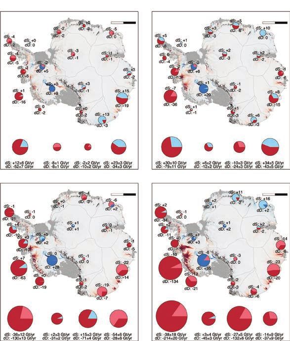
2018 was the fourth warmest year on record
              2015–2018 were the four warmest years
              on record as the long-term warming trend continues

              Ocean heat content is at a record high and
              global mean sea level continues to rise
              Artic and Antarctic sea-ice extent is
              well below average

              Extreme weather had an impact on lives and
              sustainable development on every continent

              Average global temperature reached approximately
              1 °C above pre-industrial levels
              We are not on track to meet climate change targets
              and rein in temperature increases

Every fraction of a degree of warming makes a difference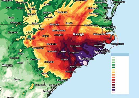
Foreword
This publication marks the twenty-fifth anni-     concentration of the major greenhouse gases,
versary of the WMO Statement on the State         the increasing rate of sea-level rise and the
of the Global Climate, which was first issued     loss of sea ice in both northern and southern
in 1994. The 2019 edition treating data for       polar regions.
2018 marks sustained international efforts
dedicated to reporting on, analysing and          The understanding of the linkage between the
understanding the year-to-year variations         observed climate variability and change and
and long-term trends of a changing climate.       associated impact on societies has also pro-
                                                  gressed, thanks to the excellent collaboration
Substantial knowledge has been produced           of sister agencies within the United Nations
and delivered annually during this period         system. This current publication includes some
to inform WMO Member States, the United           of these linkages that have been recorded in
Nations system and decision-makers about          recent years, in particular from 2015 to 2018,
the status of the climate system. It comple-      a period that experienced a strong influence
ments the Intergovernmental Panel on Climate      of the El Niño and La Niña phenomena in
Change (IPCC) five-to-seven year reporting        addition to the long-term climate changes.
cycle in producing updated information for
the United Nations Framework Convention           Global temperature has risen to close to 1 °C
for Climate Change and other climate-related      above the pre-industrial period. The time
policy frameworks.                                remaining to achieve commitments under
                                                  the Paris agreement is quickly running out.
Since the Statement was first published,
climate science has achieved an unprec-           This report will inform the United Nations
edented degree of robustness, providing           Secretary-General’s 2019 Climate Action
authoritative evidence of global temperature      Summit. I therefore take this opportunity to
increase and associated features such as          thank all the contributors – authors, National
sea-level rise, shrinking sea ice, glacier mass   Meteorological and Hydrological Services,
loss and extreme events linked to increasing      global climate data and analyses centres,
temperatures, such as heatwaves. There are        Regional Specialized Meteorological Centres,
still areas that need more observations and       Regional Climate Centres and the United
research, including assessing the contribu-       Nations agencies that have collaborated on
tion of climate change to the behaviour of        this authoritative publication.
extreme events and to ocean currents and
atmospheric jet streams that can induce
extreme cold spells in some places and mild
conditions in others.

Key findings of this Statement include
the striking consecutive record warming
recorded from 2015 through 2018, the con-                          (P. Taalas)
tinuous upward trend in the atmospheric                        Secretary-General

                                                                                                   3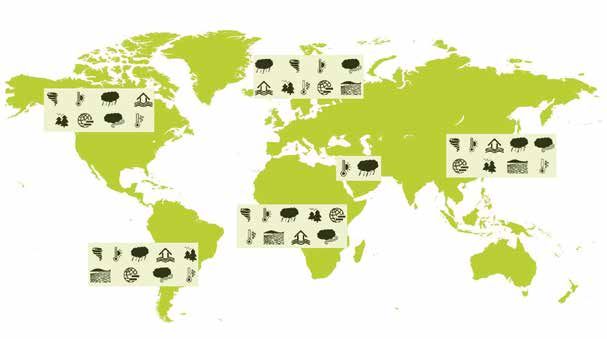
Statement by the United Nations
Secretary-General
The data released in this report give cause for we work to achieve the goals of the Paris
great concern. The past four years were the Agreement. Specifically, I am calling on all
warmest on record, with the global average leaders to come to New York in September
surface temperature in 2018 approximately with concrete, realistic plans to enhance
1 °C above the pre-industrial baseline. their nationally determined contributions by
2020 and reach net zero emissions around
These data confirm the urgency of climate mid-century. The Summit will also demon-
action. This was also emphasized by the strate transformative action in all the areas
recent Intergovernmental Panel on Climate where it is needed.
Change (IPCC) special report on the impacts
of global warming of 1.5 °C. The IPCC found There is no longer any time for delay. I commend
that limiting global warming to 1.5 °C will this report as an indispensable contribution
require rapid and far-reaching transitions in to global efforts to avert irreversible climate
land, energy, industry, buildings, transport, disruption.
and cities, and that global net human-caused
emissions of carbon dioxide need to fall by
about 45% from 2010 levels by 2030, reaching
“net zero” around 2050.
To promote greater global ambition on
addressing climate change, I am convening
a Climate Action Summit on 23 September.
The Summit aims to mobilize the neces- (A. Guterres)
sary political will for raising ambition as United Nations Secretary-General
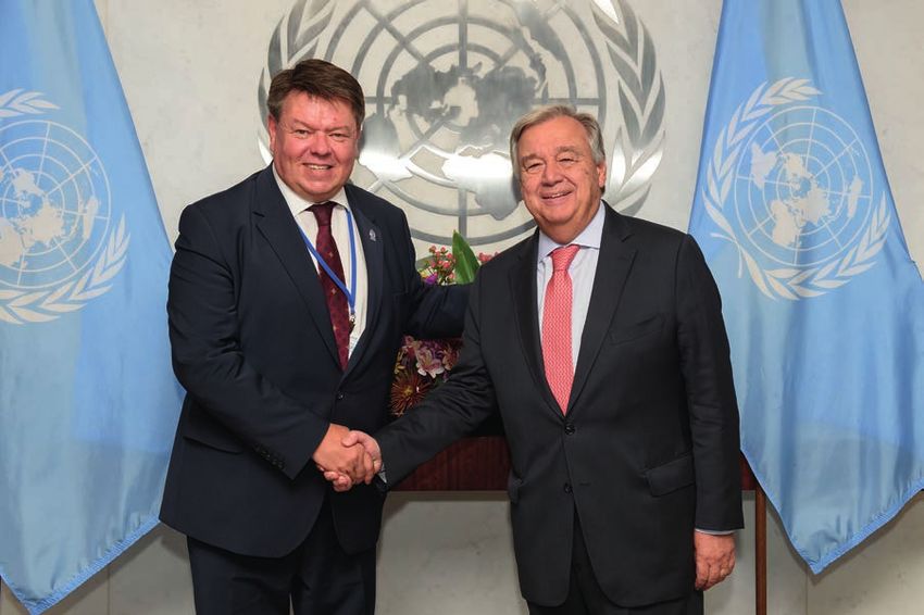
UN Photo/Loey Felipe
WMO Secretary-General Petteri Taalas (left) and United Nations Secretary-General António Guterres
during a meeting in New York in September 2018.
4
Statement by the President of the
United Nations General Assembly
             This wide ranging and significant report by the World
             Meteorological Organization clearly underlines the need
             for urgent action on climate change and shows the value
             of authoritative scientific data to inform governments in
             their decision-making process. It is one of my priorities as
             President of the General Assembly to highlight the impacts
             of climate change on achieving the sustainable develop-
             ment goals and the need for a holistic understanding of
             the socioeconomic consequences of increasingly intense
             extreme weather on countries around the world. This
             current WMO report will make an important contribution
             to our combined international action to focus attention
             on this problem.

                       María Fernanda Espinosa Garcés
               President of the United Nations General Assembly
                                  73rd Session

                                                                            5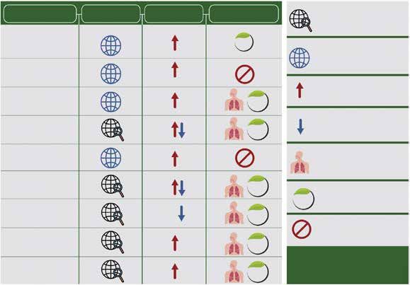
State-of-the-climate indicators
                                 TEMPERATURE                                                 0.86 °C above the pre-industrial baseline. For
Figure 1. Global mean                                                                        comparison, the average anomaly above the
temperature anomalies
                                 The global mean temperature for 2018 is                     same baseline for the most recent decade
with respect to the
1850–1900 baseline
                                 estimated to be 0.99 ± 0.13 °C above the pre-               2009–2018 was 0.93 ± 0.07 °C,1 and the aver-
for the five global              industrial baseline (1850–1900). The estimate               age for the past five years, 2014–2018, was
temperature datasets.            comprises five independently maintained                     1.04 ± 0.09 °C above this baseline. Both of
Source: UK Met Office            global temperature datasets and the range                   these periods include the warming effect of
Hadley Centre.                   represents their spread (Figure 1).                         the strong El Niño of 2015–2016.

                                                                                             Above-average temperatures were wide-
                    Global mean temperature difference from 1850–1900 (°C)                   spread in 2018 (Figure 2). According to
       1.2          HadCRUT                                                                  continental numbers from NOAA, 2018 was
                    NOAAGlobalTemp
       1.0          GISTEMP                                                                  ranked in the top 10 warmest years for Africa,
                    ERA-Interim
                    JRA-55
                                                                                             Asia, Europe, Oceania and South America.
       0.8
                                                                                             Only for North America did 2018 not rank
       0.6
                                                                                             among the top 10 warmest years, coming
 °C

       0.4                                                                                   eighteenth in the 109-year record.
       0.2

       0.0
                                                                                             There were a number of areas of notable
                                                                                             warmth. Over the Arctic, annual average
      −0.2
                                                                                             temperature anomalies exceeded 2 °C widely
             1850        1875        1900   1925          1950   1975     2000     2025      and 3 °C in places. Although Arctic tempera-
                                                   Year
                                                                                             tures were generally lower than in the record
                                                                                             year of 2016, they were still exceptionally
                                                                                             high relative to the long-term average. An
                                 The year 2018 was the fourth warmest on                     area extending across Europe, parts of North
                                 record and the past four years – 2015 to                    Africa, the Middle East and southern Asia was
                                 2018 – were the top four warmest years in                   also exceptionally warm, with a number of
                                 the global temperature record. The year 2018                countries experiencing their warmest year on
                                 was the coolest of the four. In contrast to the             record (Czechia, France, Germany, Hungary,
                                 two warmest years (2016 and 2017), 2018
                                 began with weak La Niña conditions, typically               1
                                                                                                 IPCC used NOAAGlobalTemp, GISTEMP and two versions of
                                 associated with a lower global temperature.                     HadCRUT4 for their assessment. One version of HadCRUT4
                                                                                                 was an earlier version of the one used here, the other is
                                 The IPCC special report on the impacts of                       produced by filling gaps in the data using a statistical
                                                                                                 method (Cowtan, K. and R.G. Way, 2014: Coverage bias in
                                 global warming of 1.5 °C (Global Warming
                                                                                                 the HadCRUT4 temperature series and its impact on recent
                                 of 1.5 °C) reported that the average global                     temperature trends. Quarterly Journal of the Royal Mete-
                                 temperature for the period 2006–2015 was                        orological Society, 140:1935–1944, doi:10.1002/qj.2297).

Figure 2. Surface-air
temperature anomaly
for 2018 with respect to
the 1981–2010 average.
Source: ECMWF ERA-
Interim data, Copernicus
Climate Change Service.                                                 -10 -5 -3 -2 -1 -0.5 0 0.5 1    2   3   5 10 ºC

         6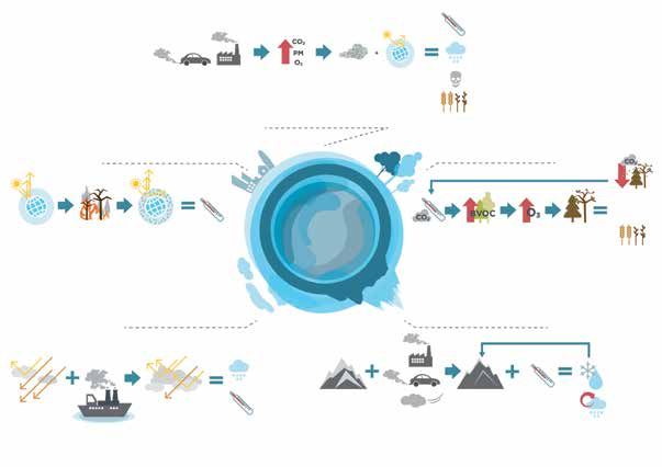
DEFINITION OF STATE OF THE CLIMATE INDICATORS

                                                                                                                             Key components of
                                                                                                                             climate system and
                                                                                                                             interactions:
                                                                                                Changes in the               energy budget,
 Changes in the energy budget               Changes in the     Changes in weather             hydrological cycle             atmospheric composition,
     Atmosphere and ocean                    atmospheric         Extreme events             river discharge, lakes,
   temperature, heat content                 composition                                         precipitation
                                                                                                                             weather, hydrological
                                                                                                                             cycle, ocean and
                                                                                                                             cryosphere.
                                                  ATMOSPHERE

                                        CO2, CH4, N2O, O3, H2O and others                               Clouds
                                                    Aerosols
                                                                                         Atmosphere-
                      Precipitation                    Volcanic Activity                   Biosphere
 Atmosphere-Ice
                      Evaporation                                                         Interaction
   Interaction
                                                                                                     Land-
                                                                                                 Atmosphere
          Heat      Wind     Terrrestrial                                                         Interaction
        Exchange    Stress   Radiation
                                                                                                          Ice Sheet

  Sea Ice                                             Glacier                         BIOSPHERE
          HYDROSPHERE
              Ocean
                                                                                              Land Surface
                                            Human Influence                                 Droughts, Floods
  Ice-Ocean
   Coupling
                                                                                     Soil Carbon

                   Rivers and
                                                                   Changes in the cryosphere
                     Lakes
                                                        Snow, Frozen Ground, Sea Ice, Ice Sheets, Glaciers

         Changes in the ocean                        Changes in and on the land surface
 Sea Level, Ocean Currents, Acidification                        Vegetation

The large number of existing indicators produced by climate scientists are useful for many
specific technical and scientific purposes and audiences. They are thus not all equally
suitable for helping non-specialists to understand how the climate is changing. Identifying
a subset of key indicators that capture the components of the climate system and their
essential changing behaviour in a comprehensive way helps non-scientific audiences to
easily understand the changes of key parameters of the climate system.

The World Meteorological Organization uses a list of seven state-of-the-climate indicators
that are drawn from the 55 Global Climate Observing System (GCOS) Essential Climate
Variables, including surface temperature, ocean heat content, atmospheric carbon dioxide
(CO2), ocean acidification, sea level, glacier mass balance and Arctic and Antarctic sea ice
extent. Additional indicators are usually assessed to allow a more detailed picture of the
changes in the respective domain. These include in particular – but are not limited to – pre-
cipitation, GHGs other than CO2, snow cover, ice sheet, extreme events and climate impacts.

                     e       era re a                                           er
                                                                                                    ea a              a er           r          ere
                             e er

                                ra e                                                                            ea
                                                                           er                                                                a er
                         e      era re                                                              a            a

                                                                                                                                         r      a
                             ea             ea                                                           ea e e                              ar
                                                                                                                                    ea       ee e

   State-of-the-climate indicators used by WMO for tracking climate variability and change at global level, including surface
    temperature, ocean heat content, atmospheric CO 2 , ocean acidification, sea level, glacier mass balance and Arctic and
              Antarctic sea-ice extent. These indicators are drawn from the 55 GCOS Essential Climate Variables.
                                  Source: https://gcos.wmo.int/en/global-climate-indicators.

                                                                                                                                                        7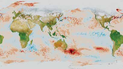
DATA SOURCES AND BASELINES FOR GLOBAL TEMPERATURE

    The assessment of global temperatures                            The period chosen as a baseline against which
    presented in the Statement is based on                           to calculate anomalies usually depends on
    five datasets. Three of these are based on                       the application. Commonly used baselines
    temperature measurements made at weather                         include the periods 1961–1990, 1981–2010 and
    stations over land and by ships and buoys                        1850–1900. The last of these is often referred to
    on the oceans, combined using statistical                        as a pre-industrial baseline. For some applica-
    methods. Each of the data centres, NOAA                          tions, for example assessing the temperature
    NCEIs,1 NASA GISS, 2 and the Met Office                          change during the twentieth century, the choice
    Hadley Centre and Climatic Research Unit at                      of baseline can make little or no difference.
    the University of East Anglia, 3 processes the
    data in different ways to arrive at the global                   The period 1961–1990 is currently rec-
    average. Two of the datasets are reanalysis                      ommended by WMO for climate change
    datasets – from ECMWF and its Copernicus                         assessments. This baseline period was used
    Climate Change Service (ERA-Interim), and                        extensively in the past three IPCC assessment
    JMA (JRA-55). Reanalyses combine millions                        reports (AR3, AR4 and AR5) and therefore
    of meteorological and marine observations,                       provides a consistent point of comparison
    including from satellites, with modelled values                  over time. Considerable effort has been made
    to produce a complete “reanalysis” of the                        to calculate and disseminate climate normals
    atmosphere. The combination of observations                      for this period.
    with models makes it possible to estimate
    temperatures at any time and in any place                        A commonly used value for the absolute
    across the globe, even in data-sparse areas                      global average temperature for 1961–1990 is
    such as the polar regions. The high degree                       14 °C. This number is not known with great
    of consistency of the global averages across                     precision, however, and may be half a degree
    these datasets demonstrates the robustness                       higher or lower. As explained previously, this
    of the global temperature record.                                margin of error for this actual temperature
                                                                     value is considerably larger than is typical for
    Global temperatures are usually expressed as                     an annually averaged temperature anomaly,
    “anomalies”, that is, temperature differences                    which is usually around 0.1 °C.
    from the average for a particular baseline
    period. Although actual temperatures can                         The 1981–2010 baseline period is used for
    vary greatly over short distances – for exam-                    climate monitoring. A recent period such as
    ple, the temperature difference between the                      this one is often preferred because it is most
    top and bottom of a mountain – temperature                       representative of current or “normal” condi-
    anomalies are representative of much wider                       tions. These 30-year averages are, indeed,
    areas. That is, if it is warmer than normal at                   often referred to as “climate normals”. Using
    the top of the mountain, it is probably warmer                   a 1981–2010 normal means that it is possible
    than normal at the bottom of it. Averaged                        to use data from satellite instruments and
    over a month, coherent areas of above- or                        reanalyses for comparison, which do not
    below-average temperature anomalies can                          often extend much further back in time. The
    extend for thousands of kilometres. To get                       1981–2010 period is around 0.3 °C warmer
    a reasonable measurement of the global                           than 1961–1990.
    temperature anomaly, one needs only a few
    stations within each of these large coherent                     The period 1850–1900 was used to represent
    areas. On the other hand, obtaining an accu-                     “pre-industrial” conditions in the IPCC Global
    rate measurement of the actual temperature                       Warming of 1.5 °C report and is the period
    requires far more stations and careful, repre-                   adopted in this Statement. Monitoring global
    sentative sampling of many different climates.                   temperature differences from pre-industrial
                                                                     conditions is important because the Paris
                                                                     Agreement seeks to limit global warming to
                                                                     1.5 °C or 2 °C above pre-industrial conditions.
    1
        NOA A NCEI produce and maintain global temperature
        datasets called NOAAGlobalTemp.
                                                                     The downside of using this baseline are that
                                                                     there are relatively few observations from
    2
        NASA GISS produces and maintains a global temperature
        dataset called GISTEMP.                                      this time and consequently there are larger
    3
        The UK Met Office Hadley Centre and Climatic Research
                                                                     uncertainties associated with this choice.
        Unit at the University of East Anglia produce and maintain   The 1850–1900 period is around 0.3 °C cooler
        a global temperature dataset called HadCRUT4.                than 1961–1990.

8
Serbia, Switzerland) or one in the top five globally averaged mole fractions of CO2 at
(Belgium, Estonia, Israel, Latvia, Pakistan, 405.5 ± 0.1 parts per million (ppm), methane
the Republic of Moldova, Slovenia, Ukraine). (CH4) at 1 859 ± 2 parts per billion (ppb) and
For Europe as a whole, 2018 was one of the nitrous oxide (N2O) at 329.9 ± 0.1 ppb (Figure 3).
three warmest years on record. Other areas of These values constitute, respectively, 146%,
notable warmth included the south-western 257% and 122% of pre-industrial levels (before
United States, eastern parts of Australia (for 1750). Global average figures for 2018 will
the country overall it was the third warmest not be available until late 2019, but real-time Figure 3. Top row:
year) and New Zealand, where it was the joint data from a number of specific locations, Globally averaged mole
second warmest year on record. including Mauna Loa (Hawaii) and Cape Grim fraction (measure of
(Tasmania) indicate that levels of CO2, CH4 and concentration) from
In contrast, areas of below-average tempera- N2O continued to increase in 2018. The IPCC 1984 to 2017 of CO 2 (ppm;
tures over land were more limited. Parts of Global Warming of 1.5 °C report found that left), CH 4 (ppb; centre)
and N 2 O (ppb; right). The
North America and Greenland, central Asia, limiting warming to 1.5 °C above pre-industrial
red line is the monthly
western parts of North Africa, parts of East temperatures implies reaching net zero CO2
mean mole fraction
Africa, coastal areas of western Australia and emissions globally around 2050, and this with with the seasonal
western parts of tropical South America were concurrent deep reductions in emissions of variations removed; the
cooler than average, but not unusually so. non-CO2 forcers, particularly CH4. blue dots and line show
the monthly averages.
GREENHOUSE GASES AND OZONE CARBON BUDGET Bottom row: Growth
rates representing
increases in successive
Increasing levels of GHGs in the atmosphere Accurately assessing CO2 emissions and their
annual means of mole
are key drivers of climate change. Atmospheric redistribution within the atmosphere, oceans,
fractions for CO 2 (ppm
concentrations reflect a balance between and land – the “global carbon budget” – helps per year; left), CH 4 (ppb
sources (including emissions due to human us capture how humans are changing the per year; centre) and
activities) and sinks (for example, uptake Earth’s climate, supports the development N 2 O (ppb per year; right).
by the biosphere and oceans). In 2017, GHG of climate policies, and improves projections Source: WMO Global
concentrations reached new highs, with of future climate change. Atmosphere Watch.
410 1900 335
CO 2 mole fraction (ppm)
N2O mole fraction (ppb)
CH 4 mole fraction (ppb)
400 1850 330
390 325
1800
380 320
1750
370 315
1700
360 310
350 1650 305
340 1600 300
1985 1990 1995 2000 2005 2010 2015 1985 1990 1995 2000 2005 2010 2015 1985 1990 1995 2000 2005 2010 2015
Year Year Year
4.0 20 2.0
CO 2 growth rate (ppm/yr)
CH 4 growth rate (ppb/yr)
N2O growth rate (ppb/yr)
15
3.0 1.5
10
2.0 1.0
5
1.0 0.5
0
0.0 -5 0.0
1985 1990 1995 2000 2005 2010 2015 1985 1990 1995 2000 2005 2010 2015 1985 1990 1995 2000 2005 2010 2015
Year Year Year
9Coastal blue carbon
Kirsten Isensee,1 Jennifer Howard, 2 Emily Pidgeon, 2 Jorge Ramos, 2
1
IOC-UNESCO, France
2
Conservation International, United States
In broad terms, “blue carbon” refers to carbon stored, sequestered and cycled through
coastal and ocean ecosystems. However, in climate mitigation, coastal blue carbon (also
known as “coastal wetland blue carbon”)1 is defined as the carbon stored in mangroves,
tidal salt marshes, and seagrass meadows within the soil; the living biomass above ground
(leaves, branches, stems); the living biomass below ground (roots and rhizomes); and the
non-living biomass (litter and dead wood)2 (see table). When protected or restored, coastal
blue carbon ecosystems act as carbon sinks (see figure (a)).They are found on every con-
tinent except Antarctica and cover approximately 49 Mha.
Currently, for a blue carbon ecosystem to be recognized for its climate mitigation value within
international and national policy frameworks it is required to meet the following criteria:
(a) Quantity of carbon removed and stored or prevention of emissions of carbon by the
ecosystem is of sufficient scale to influence climate;
(b) Major stocks and flows of GHGs can be quantified;
(c) Evidence exists of anthropogenic drivers impacting carbon storage or emissions;
(d) Management of the ecosystem that results in increased or maintained sequestration
or emission reductions is possible and practicable;
(e) Management of the ecosystem is possible without causing social or environmental
harm.
However, the ecosystem services provided by mangroves, tidal marshes and seagrasses
are not limited to carbon storage and sequestration. They also support improved coastal
water quality, provide habitats for economically important fish species, and protect coasts
against floods and storms. Recent estimates revealed that mangroves are worth at least
US$ 1.6 billion each year in ecosystem services.
Despite the proven importance for ocean health and human well-being, mangroves, tidal
marshes and seagrasses are being lost at a rate of up to 3% per year (see table). When
degraded or destroyed, these ecosystems emit the carbon they have stored for centuries
into the ocean and atmosphere and become sources of GHGs (see figure, (b)).
Based on IPCC data it is estimated that as much as a billion tons of CO2 are being released
annually from degraded coastal blue carbon ecosystems (from all three systems – man-
groves, tidal marshes and seagrasses), which is equivalent to 19% of emissions from tropical
deforestation globally.3
CO2 (a) (b)
Anthropogenic GHG emissions
CO2
Sequestration
into woody CO2
biomass
CO2
CO2 CO2
Carbon uptake Carbon released
by photosynthesis through respiration
and decomposition
Sequestration
into soil
Carbon sequestration and release in intact and degraded coastal ecosystems – (a): In intact coastal wetlands (from left to right:
mangroves, tidal marshes and seagrasses), carbon is taken up via photosynthesis (purple arrows) and sequestered in the long
term into woody biomass and soil (red dashed arrows) or respired (black arrows). (b): When soil is drained from degraded
coastal wetlands, the carbon stored in the soils is consumed by microorganisms, which respire and release CO 2 as a metabolic
waste product. This happens at an increased rate when the soils are drained and oxygen is more available, which leads to
greater CO 2 emissions. The degradation, drainage and conversion of coastal blue carbon ecosystems from human activity (that
10 is, deforestation and drainage, impounded wetlands for agriculture, dredging) result in a reduction in CO 2 uptake due to the loss
of vegetation (purple arrows) and the release of globally important GHG emissions.Carbon storage potential of coastal and marine ecosystems1
Mangroves Tidal marsh Seagrass
Geographic extent (million hectares) 13.8–15.24,5 2.2–40 6,7 30–60 6
Sequestration rate (Mg C ha -1 yr-1) 2.26 ± 0.39 6 2.18 ± 0.24 6 1.38 ± 0.38 6
Total carbon sequestered annually
(extent x sequestration rate) 31.2–34.4 4.8–87.2 41.4–82.8
(Million Mg C yr-1)
Mean global Top metre of soil
280 8 250 8 140 8
estimate of pool (Mg C ha -1)
carbon stock
Biomass pool
(total = (soil 1278 98 28
(Mg C ha -1)
+ biomass) x
extent) Total (million Mg C) 5 617–6 186 570–10 360 4 260–8 520
Centuries to Centuries to Centuries to
Carbon stock stability (Years)
millennium millennium millennium
Anthropogenic conversion rate (% yr-1) 0.7–3.0 9 1.0–2.010,11 0.4–2.612,13
Potential emissions due to
anthropogenic conversion assuming all
carbon is converted to CO2 ((total carbon 144.3–681.1 20.9–760.4 62.5–813.0
stock per ha x ha converted annually)
x 3.67 (conversion rate to CO2))
1
Howard, J., A. Sutton-Grier, D. Herr, J. Kleypas, E. Landis, E. Mcleod, E. Pidgeon and S. Simpson, 2017: Clarifying the role
of coastal and marine systems in climate mitigation. Frontiers in Ecology and the Environment, 15(1):42–50, doi:10.1002/
fee.1451.
2
Howard, J., S. Hoyt, K. Isensee, M. Telszewski and E. Pidgeon (eds), 2014: Coastal Blue Carbon: Methods for Assessing
Carbon Stocks and Emissions Factors in Mangroves, Tidal Salt Marshes, and Seagrasses. Conservation International,
IOC-UNESCO, International Union for Conservation of Nature. Arlington, Virginia, United States.
3
Intergovernmental Panel on Climate Change, 2006: 2006 Guidelines for National Greenhouse Gas Inventories. (H.S. Eggleston,
L. Buendia, K. Miwa, T. Ngara and K. Tanabe, eds). Prepared by the National Greenhouse Gas Inventories Programme.
Kanagawa, Japan, IGES.
4
Giri, C., et al., 2011: Status and distribution of mangrove forests of the world using Earth observation satellite data. Global
Ecology and Biogeography, 20:154–59.
5
Spalding, M., M. Kainuma and L. Collins, 2010: World Atlas of Mangroves. London and Washington, D.C., Earthscan.
6
Mcleod, E., G.L. Chmura, S. Bouillon, R. Salm, M. Björk, C.M. Duarte, C.E. Lovelock, W.H. Schlesinger and B.R. Silliman, 2011:
A blueprint for blue carbon: toward an improved understanding of the role of vegetated coastal habitats in sequestering
CO 2 . Frontiers in Ecology and the Environment, 9(10):552–560, doi:10.1890/110004.
7
Duarte, C.M., et al., 2013: The role of coastal plant communities for climate change mitigation and adaptation. Nature
Climate Change, 3:961–68.
8
Pendleton, L., et al., 2012: Estimating global “blue carbon” emissions from conversion and degradation of vegetated coastal
ecosystems. PLoS ONE, 7(9):e43542.
9
Food and Agriculture Organization of the United Nations, 2007: The World’s Mangroves 1980–2005. FAO Forestry Paper
153. Rome, FAO.
10
Duarte, C.M., J. Borum, F.T. Short and D.I. Walker, 2005: Seagrass ecosystems: their global status and prospects. In: Aquatic
Ecosystems: Trends and Global Prospects (N.V.C. Polunin, ed.). Cambridge, United Kingdom, Cambridge University Press.
11
Bridgham, S. D., J.P. Megonigal, J.K. Keller, N.B. Bliss and C. Trettin, 2006: The carbon balance of North American wetlands.
Wetlands, 26(4):889–916.
12
Waycott, M., et al., 2009: Accelerating loss of seagrasses across the globe threatens coastal ecosystems. Proceedings
of the National Academy of Sciences of the United States of America, 106:12377–12381.
11
13
Green, E.P. and F.T. Short (eds), 2003: World Atlas of Seagrasses. Berkeley, University of California Press.Figure 4
(a) Annual global carbon The rise in atmospheric CO2 causes climate change (a)
budget averaged for The global carbon cycle 2008-2017
the decade 2008–2017. Fossil CO2 Land-use change Biosphere Atmospheric CO2 Ocean
Anthropogenic
Fluxes are in billion tons fluxes 2008-2017
average GtCO2 per year
of CO 2 . Circles show 5 +17.3
(3-8)
carbon stocks in billion 0.5 Atmospheric CO2 9
12 (7-11)
tons of carbon. Carbon cycling GtCO2
per year (9-14)
34 440
(b) The historical global (33-36)
carbon budget, 1900– Stocks available GtCO2
330
440 Vegetation
2017. Carbon emissions 4000
are partitioned among 140,000
Gas reserves 330
the atmosphere and Permafrost
Organic
Marine
biota
Oil reserves Soils Dissolved
Surface carbon
carbon sinks on land sediments inorganic
Coal reserves carbon
and in the oceans. The
“imbalance” between Bu
udget imbalance +2
total emissions and total
Copyright: Produced by the Future Earth Media Lab for the Global Carbon Project. http://www.globalcarbonproject.org/carbonbudget/index.htm.
sinks reflects the gaps Written and edited by Corinne Le Quéré (Tyndall Centre UEA) with the Global Carbon Budget team. Impacts based on IPCC SR15.
Graphic by Nigel Hawtin. Credits: Le Quéré et al. Earth System Science Data (2018);
in data, modelling or our NOAA-ESRL and the Scripps Institution of Oceanography; Illustrative projections by D. van Vuuren based on the IMAGE model
understanding of the
carbon cycle.
Source: Global Carbon Fossil CO2 emissions have grown almost con- emissions reached an estimated 41.5 ± 3.0 bil-
Project, http://www. tinuously for the past two centuries (Figure 4), lion tons of CO2 in 2018.
globalcarbonproject.org/ a trend only interrupted briefly by globally
carbonbudget; Le Quéré, significant economic downturns. Emissions The continued high emissions have led to high
et al., 2018. 2 to date continued to grow at 1.6% in 2017 and levels of CO2 accumulation in the atmosphere
at a preliminary 2.0% (1.1%–3.4%) per year in that amounted to 2.82 ± 0.09 ppm in22018. 3
2018. It is anticipated that a new record high This level of atmospheric CO2 is the result of
of 36.9 ± 1.8 billion tons of CO2 was reached the accumulation of only a part of the total CO2
in 2018. emitted because about 55% of all emissions
are removed by CO2 sinks in the oceans and
Net CO2 emissions from land use and land terrestrial vegetation.
cover changes were on average 5.0 ± 2.6 bil-
lion tons per year over the past decade, with Sinks for CO2 are distributed across the hemi-
highly uncertain annually resolved estimates. spheres, on land and oceans, but CO2 fluxes
Together, land-use change and fossil CO 2 in the tropics (30°S–30°N) are close to carbon
neutral due to the CO2 sink being largely offset
by emissions from deforestation. Sinks for
CO2 in the southern hemisphere are domi-
Balance of sources and sinks (b) nated by the removal of CO2 by the oceans,
40 while the stronger sinks in the northern hemi-
sphere have similar contributions from both
30 land and oceans.
Fossil
20 carbon OZONE
CO2 flux (Gt CO2/yr)
10
Land-use Following the success of the Montreal Proto-
0 change col, the use of halons and chlorofluorocarbons
Ocean sink (CFCs) has been discontinued. However, due
−10
to their long lifetime these compounds will
Land sink
−20 remain in the atmosphere for many decades.
Total estimated sources do There is still more than enough chlorine and
−30 not match total estimated
sinks. This imbalance reflects Atmosphere
the gap in our understanding.
−40
2
Le Quéré, et al., 2018: Global carbon budget 2018. Earth
System Science Data, 10:2141–2194; and March 2019 updates.
1900 1920 1940 1960 1980 2000 2017 3
NOAA, 2019: Trends in atmospheric carbon dioxide, https://
Global Carbon Project • Data:Year
CDIAC/GCP/NOAA-ESRL/UNFCCC/BP/USGS
www.esrl.noaa.gov/gmd/ccgg/trends/gl_gr.html.
12bromine present in the atmosphere to cause 30 Figure 5. Area (10 6 km 2 )
1979-2017
complete destruction of ozone at certain alti- Ozone hole area 2014 where the total ozone
tudes in Antarctica from August to December, 25 2015
2016
column is less than 220
so the size of the ozone hole from one year 2017 Dobson units. The dark
2018
20 green-blue shaded area
to the next is to a large degree governed by
is bounded by the 30 th
Area (106 km2)
meteorological conditions. 15 and 70 th percentiles
and the light green-
In 2018, south polar stratospheric tem- 10 blue shaded area is
peratures were below the long-term mean bounded by the 10 th and
(1979–2017), and the stratospheric polar vor- 5 90 th percentiles for the
tex was relatively stable with less eddy heat period 1979–2017. The
flux than the average from June to mid-No- 0
Jul Aug Sep Oct Nov Dec
thin black lines show the
Month maximum and minimum
vember. Ozone depletion started relatively
values for each day
early in 2018 and remained above the long- during the 1979–2017
term average until about mid-November period. Source: based
(Figure 5). exceeded 4 °C above normal at certain times on data from the NASA
(Figure 6). The record high sea-surface tem- Ozone Watch website
The ozone hole area reached its maximum for peratures were linked to unusually warm (Ozone Mapping and
2018 on 20 September, with 24.8 million km2, conditions over New Zealand, which had Profiler Suite, Ozone
whereas it reached 28.2 million km 2 on its warmest summer and warmest month Monitoring Instruments
and Total Ozone Mapping
2 October in 2015 and 29.6 million km2 on (January) on record. It was also the warmest
Spectrometer).
24 September 2006 according to an analysis November to January period on record for
from NASA. Despite a relatively cold and Tasmania. The warm waters were associated
stable vortex, the 2018 ozone hole was smaller with high humidity and February, though past
than in earlier years with similar temperature the peak of the marine heatwave, saw a num-
conditions, such as, for example, 2006. This ber of extreme rainfall events in New Zealand.
is an indication that the size of the ozone
hole is starting to respond to the decline OCEAN HEAT CONTENT
in stratospheric chlorine as a result of the
provisions of the Montreal Protocol. More than 90% of the energy trapped by
GHGs goes into the oceans and ocean heat
content provides a direct measure of this
Figure 6. Daily sea-
THE OCEANS energy accumulation in the upper layers of the
surface temperature
ocean. Unlike surface temperatures, where anomalies for 29 January
SEA-SURFACE TEMPERATURES the incremental long-term increase from one 2018 with respect to the
year to the next is typically smaller than the 1987–2005 average.
Sea-surface waters in a number of ocean year-to-year variability caused by El Niño and Source: UK Met Office
areas were unusually warm in 2018, including La Niña, ocean heat content is rising more Hadley Centre
much of the Pacific with the exception of the
eastern tropical Pacific and an area to the
north of Hawaii, where temperatures were Sea-surface Temperature difference from 1987–2005 (ºC)
below average. The western Indian Ocean, -5 -4 -3 -2 -1 0 1 2 3 3 5
tropical Atlantic and an area of the North
Atlantic extending from the east coast of
the United States were also unusually warm.
Unusually cold surface waters were observed
in an area to the south of Greenland, which
is one area of the world that has seen long-
term cooling.
In November 2017, a marine heatwave devel-
oped in the Tasman Sea that persisted until
February 2018. Sea-surface temperatures in
the Tasman Sea exceeded 2 °C above normal
widely and daily sea-surface temperatures
13Deoxygenation of open ocean and
coastal waters
IOC Global Ocean Oxygen Network change is expected to further amplify deoxy-
(GO2NE), Kirsten Isensee,1 genation in coastal areas, already influenced by
Denise Breitburg, 2 Marilaure Gregoire3 anthropogenic nutrient discharges, by decreas-
ing oxygen solubility, reducing ventilation by
1
IOC-UNESCO, France strengthening and extending periods of sea-
2
Smithsonian Environment Research Center, sonal stratification of the water column, and in
United States some cases where precipitation is projected to
3
University of Liège, Belgium increase, by increasing nutrient delivery.
Both observations and numerical models indicate The volume of anoxic regions of the ocean oxy-
that oxygen is declining in the modern open and gen minimum zones has expanded since 1960,2
coastal oceans, including estuaries and semi-en- altering biogeochemical pathways by allowing
closed seas. Since the middle of the last century, processes that consume fixed nitrogen and
there has been an estimated 1%–2% decrease release phosphate, iron, hydrogen sulfide (H2S),
(that is, 2.4–4.8 Pmol or 77 billion–145 billion and possibly N2O (see figure). The relatively
tons) in the global ocean oxygen inventory,1, 2 limited availability of essential elements, such
while, in the coastal zone, many hundreds of sites as nitrogen and phosphorus, means such alter-
are known to have experienced oxygen concen- ations are capable of perturbing the equilibrium
trations that impair biological processes or are chemical composition of the oceans. Further-
lethal for many organisms. Regions with histori- more, we do not know how positive feedback
cally low oxygen concentrations are expanding, loops (for example, remobilization of phosphorus
and new regions are now exhibiting low oxygen and iron from sediment particles) may speed
conditions. While the relative importance of up the perturbation of this equilibrium.
the various mechanisms responsible for the
Deoxygenation affects many aspects of the
loss of the global ocean oxygen content is not
ecosystem services provided by the world’s
precisely known, global warming is expected
oceans and coastal waters. For example, the
to contribute to this decrease directly because
process affects biodiversity and food webs,
the solubility of oxygen decreases in warmer
Oxygen minimum zones and can reduce growth, reproduction and sur-
waters, and indirectly through changes in ocean
(blue) and areas with vival of marine organisms. Low-oxygen-related
dynamics that reduce ocean ventilation, which is
coastal hypoxia (red) changes in spatial distributions of harvested
in the world’s oceans. the introduction of oxygen to the ocean interior.
species can cause changes in fishing locations
Coastal hypoxic sites Model simulations have been performed for the
and practices, and can reduce the profitability of
mapped here are end of this century that project a decrease of
fisheries. Deoxygenation can also increase the
systems where oxygen oxygen in the open ocean under both high- and
difficulty of providing sound advice on fishery
concentrations of low-emission scenarios.
< 2 mg/L have been management.
recorded and in which In coastal areas, increased export by rivers
anthropogenic nutrients of nitrogen and phosphorus since the 1950s
are a major cause of
has resulted in eutrophication of water bodies
oxygen decline. Sources:
worldwide. Eutrophication increases oxygen 1
Bopp, L., L. Resplandy, J.C. Orr, S.C. Doney, J.P. Dunne,
data from (3) and Diaz,
J.R., unpublished; figure consumption and, when combined with low M. Gehlen, P. Halloran, C. Heinze, T. Ilyina and R. Seferian,
ventilation, leads to the occurrence of oxy- 2013: Multiple stressors of ocean ecosystems in the 21st
adapted after (4), (5) century: projections with CMIP5 models. Biogeosciences,
and (6). gen deficiencies in subsurface waters. Climate 10:6225–6245.
2
Schmidtko, S., L. Stramma and M. Visbeck, 2017: Decline in
global oceanic oxygen content during the past five decades.
Nature, 542:335–339.
3
Diaz, R.J. and R. Rosenberg, 2008: Spreading dead zones and
consequences for marine ecosystems. Science, 321:926–929.
4
Isensee, K., L.A. Levin, D.L. Breitburg, M. Gregoire, V. Garçon and
L. Valdés, 2015: The ocean is losing its breath. Ocean and Climate,
Scientific Notes. http://www.ocean-climate.org/wp-content/
uploads/2017/03/ocean-out-breath_07-6.pdf.
5
Breitburg, D., M. Grégoire and K. Isensee (eds), 2018: The
Ocean is Losing Its Breath: Declining Oxygen in the World’s
Ocean and Coastal Waters. Global Ocean Oxygen Network.
IOC Technical Series No. 137. IOC-UNESCO.
6
Breitburg, D., et al., 2018: Declining oxygen in the global ocean
Hypoxic areas and coastal waters. IOC Global Ocean Oxygen Network.
0.05 0.25 1.4 mg l–1 O2
Science, 359(6371):p.eaam7240.
14Warming trends in the southern ocean
Neil Swart,1 Michael Sparrow 2 a b
0 2.0 6.0 12.014.0 18.0 .0
34.6
35
16.0
34.2 34 35.2 35.4
4.0
.0
8.0
1
Environment Canada 500
10.0
34
.4
34.8
Observations
Depth (m)
2
WMO 1,000 34.6
The greatest rates of ocean warming are in the 1,500
southern ocean, with warming reaching to the 2,000
deepest layers. However, there are significant c d
0
regional differences. The subpolar surface 6.0 12.0 16.0 18.0 34.0 34.8
.6
8. 14.0
CanESM2 (subsampled)
34.2
34
4.0
0
ocean south of the Antarctic circumpolar 10.0 34.4
34.4
500
current (ACC) has exhibited delayed warming,
Depth (m)
34.6
2.0
1,000
or even a slight cooling over past decades.1, 2
To the north of the ACC (approximately 30°S 1,500
.8
34
to 60°S), however, the southern ocean has 2,000 2.0
experienced rapid warming from the surface e f
to a depth of 2 000 m (see figure) at rates of 0 6.0
8.
12.0 16.0 18.0
14.0 34.0 34
.2
4.0
0
roughly twice those of the global ocean. 3, 4, 5
34.6
10.0 34.4
500 34.4
CanESM2 (full)
The pattern of delayed warming to the south,
Depth (m)
34.6
2.0
1,000
and enhanced surface to intermediate-depth
warming to the north is driven by the north- 1,500 34.8
ward and downward advection of heat by
2,000 2.0
the southern ocean meridional overturning 60° S 55° S 50° S 45° S 40° S 35° S 60° S 55° S 50° S 45° S 40° S 35° S
circulation.1, 2 This transfer of heat from the Latitude Latitude
surface to the interior makes the southern
–0.60 –0.20 0.20 0.60 –0.03 –0.01 0.01 0.03
ocean the primary region of anthropogenic ∆T (°C) ∆Salinity (psu)
heat uptake. 6 Indeed, the observed rapid
warming north of the ACC has been formally
attributed to increasing GHG concentrations.3 4
Gille, S.T., 2002: Warming of the Southern Ocean since Observed changes in
Changes in the westerly winds, and resulting the 1950s. Science, 295(5558):1275–1277, DOI: 10.1126/ temperature (left) and
anomalous northward Ekman transport of science.1065863. salinity (right) between
cold waters, driven by stratospheric ozone the 2006–2015 mean and
5
Gille, S.T., 2008: Decadal-scale temperature trends in the
depletion, may also contribute to the sub- the 1950–1980 mean.
southern hemisphere ocean. Journal of Climate, 21:4749–
polar surface cooling7, 8 and warming to the 4765, https://doi.org/10.1175/2008JCLI2131.1. The top panels (a, b) are
north. 3 Finally, the deep (> 2 000 m) and from observations and
abyssal (> 4 000 m) southern ocean has been
6
Roemmich, D., J. Church, J. Gilson, D. Monselesan, P. Sutton the bottom two from
and S. Wijffels, 2015: Unabated planetary warming and models, sub-sampled to
warming significantly faster than the global its ocean structure since 2006. Nature Climate Change, match the observational
mean. 9, 10 This is thought to be connected 5(3):240–245. coverage (c, d) and the
to changes in the rate of Antarctic bottom ensemble mean forcing
water formation and the lower limb of the
7
Kostov, Y., D. Ferreira, K.C. Armour and J. Marshall, 2018:
with full sampling (e, f).
Contributions of greenhouse gas forcing and the southern
meridional overturning circulation. annular mode to historical southern ocean surface tempera- The observed changes
ture trends. Geophysical Research Letters, 45:1086–1097, are primarily attributable
https://doi.org/10.1002/2017GL074964. to increases in GHGs.
Source: (3).
8
Ferreira, D., J. Marshall, C.M. Bitz, S. Solomon and A.
Plumb, 2015: Antarctic ocean and sea ice response to ozone
depletion: A two-time-scale problem. Journal of Climate,
1
Sallée, J.B., 2018: Southern ocean warming. Oceanography, 28:1206–1226, https://doi.org/10.1175/JCLI-D-14-00313.1.
31(2):52–62, https://doi.org/10.5670/oceanog.2018.215. 9
Desbruyères, D.G., S.G. Purkey, E.L. McDonagh, G.C. Johnson
2
Armour, K.C., J. Marshall, J.R. Scott, A. Donohoe and E.R. and B.A. King, 2016: Deep and abyssal ocean warming from
Newson, 2016: Southern Ocean warming delayed by cir- 35 years of repeat hydrography. Geophysical Research
cumpolar upwelling and equatorward transport. Nature Letters, 43:10356–10365.
Geoscience, 9:549–554, https://doi.org/10.1038/ngeo2731. 10
Purkey, S.G. and G.C. Johnson, 2010: Warming of global
3
Swart, N.C., S.T. Gille, J.C. Fyfe and N.P. Gillett, 2018: Recent abyssal and deep southern ocean waters between the
southern ocean warming and freshening driven by green- 1990s and 2000s: Contributions to global heat and sea level
house gas emissions and ozone depletion. Nature Geoscience, rise budgets. Journal of Climate, 23:6336–6351, https://doi.
11:836–842, https://doi.org/10.1038/s41561-018-0226-1. org/10.1175/2010JCLI3682.1.
15revealed by satellite altimetry (World Climate
Levitus
EN4
Research Programme Global Sea Level Bud-
10 get Group, 2018).5
5
Assessing the sea-level budget helps to quan-
1022 joules
0
tify and understand the causes of sea-level
change. Closure of the total sea-level budget
−5 means that the observed changes of global
mean sea level as determined from satellite
−10 altimetry equal the sum of observed con-
tributions from changes in ocean mass and
1950 1960 1970 1980 1990 2000 2010 2020 thermal expansion (based on in situ tempera-
Year
ture and salinity data, down to 2 000 m since
2005 with the international Argo project).
Figure 7. Global ocean steadily with less pronounced year-to-year Ocean mass change can be either derived
heat content change fluctuations (Figure 7). Indeed, 2018 set new from GRACE satellite gravimetry (since 2002)
(x 10 22 J) for the 0–700 m records for ocean heat content in the upper or from adding up individual contributions
layer relative to the 700 m (data since 1955) and upper 2 000 m from glaciers, ice sheets and terrestrial water
1981–2010 baseline. The
(data since 2005), exceeding previous records storage (Figure 8, right). Failure to close the
lines show annual means
from the Levitus analysis
set in 2017. sea-level budget would indicate errors in
produced by NOAA NCEI some of the components or contributions
and the EN4 analysis SEA LEVEL from components missing from the budget.
produced by the UK Met
Office Hadley Centre. Sea level is one of the seven key indicators of OCEAN ACIDIFICATION
Source: UK Met Office global climate change highlighted by GCOS 4
Hadley Centre, prepared and adopted by WMO for use in character- In the past decade, the oceans have absorbed
using data also from
izing the state of the global climate in its around 30% of anthropogenic CO 2 emis-
NOAA NCEI.
annual statements. Sea level continues to sions. Absorbed CO2 reacts with seawater and
rise at an accelerated rate (see Figure 8, left). changes ocean pH. This process is known as
Global mean sea level for 2018 was around ocean acidification. Changes in pH are linked
3.7 mm higher than in 2017 and the highest to shifts in ocean carbonate chemistry that
on record. Over the period January 1993 to can affect the ability of marine organisms,
December 2018, the average rate of rise was such as molluscs and reef-building corals,
3.15 ± 0.3 mm yr-1, while the estimated accel- to build and maintain shells and skeletal
eration was 0.1 mm yr-2. Accelerated ice mass material. This makes it particularly import-
loss from the ice sheets is the main cause ant to fully characterize changes in ocean
of the global mean sea-level acceleration as
5
World Climate Research Programme Global Sea Level Budget
Figure 8. Left: Global 4
Global climate indicators, ht tps: //gcos.wmo.int /en/ Group, 2018: Global sea-level budget 1993–present. Earth
mean sea level for
global-climate-indicators. Systems Science Data, 10:1551–1590.
the period 1993–2018
from satellite altimetry
datasets. The thin ESA climate change initiative (SL_cci) data 140 CCI GMSL
Sum of SLBC-CCI V2 components
black line is a quadratic AVISO plus near real time Jason-3 data Residual: CCI GMSI: Sum of components
Steric Dieng et al., 2017 with deep ocean included
GlaciersV2
120 Greenland ice sheet altimetry based V2
function representing Antarctic ice sheet altimetry based V2
MeanTWSV2
the acceleration. 100
Right: Contribution of
Sea level (mm)
E 80
individual components E
to the global mean sea > 60
Cl)
level during the period
..........-·...... ..,.,:.·. .................: ... . . .� ..._. ·.. .,,.......... . .......... �....
•
co
�--.·
.
• •· ,... •.. .,_. ... ./w:-L••♦ ......:-.,,,.: ....\•••••••♦•♦- 4 I • .. -- •
....
... ♦ ♦
♦ ♦
#t.
Cl)
---
(f) 40
1993–2016. Shaded
_
area around the red and 20
blue curves represents
the uncertainty range. ---
- -"' J"'r-
Source: European Space -20
Agency Climate Change 1993 1995 1997 1999 2001 2003 2005 2007 2009 2011 2013 2015 2017
Year Year
Initiative.
16carbonate chemistry. Observations in the Development Goal indicator 14.3.1 (“Average
open ocean over the last 30 years have shown marine acidity (pH) measured at agreed suite
a clear trend of decreasing pH (Figure 9). The of representative sampling stations”) will lead
IPCC AR5 reported a decrease in the surface to an expansion in the observation of ocean
ocean pH of 0.1 units since the start of the acidification on a global scale.
industrial revolution (1750). Trends in coastal
locations, however, are less clear due to the
highly dynamic coastal environment, where THE CRYOSPHERE
a great many influences such as temperature
changes, freshwater runoff, nutrient influx, The cryosphere component of the Earth sys-
biological activity and large ocean oscillations tem includes solid precipitation, snow cover,
affect CO2 levels. To characterize the variabil- sea ice, lake and river ice, glaciers, ice caps,
ity of ocean acidification, and to identify the ice sheets, permafrost and seasonally frozen
drivers and impacts, a high temporal and ground. The cryosphere provides key indica-
spatial resolution of observations is crucial. tors of climate change, yet is one of the most
under-sampled domains of the Earth system.
In line with previous reports and projections There are at least 30 cryospheric properties
on ocean acidification, global pH levels con- that, ideally, would be measured. Many are
tinue to decrease. More data for recently measured at the surface, but spatial coverage
established sites for observations in New is generally poor. Some have been measured
Zealand show similar patterns, while filling for many years from space; the capability to
important data gaps for ocean acidification measure others with satellites is developing.
in the southern hemisphere. Availability of The major cryosphere indicators for the state
operational data is currently limited, but it of the climate include sea ice, glaciers, and the
is expected that the newly introduced meth- Greenland ice sheet. Snow cover assessment
odology for the United Nations Sustainable is also included in this section.
Hawaii Ocean Time Series Hawaii Ocean Time Series
475 8.20
450
8.15
425
pHTOT (in situ)
pCO2 (μatm)
400 8.10
375
350 8.05
325
8.00
300
275 7.95
1990 1995 2000 2005 2010 2015 1990 1995 2000 2005 2010 2015
Year Year
Figure 9. Records
Bermuda Atlantic Time Series Bermuda Atlantic Time Series of pCO 2 and pH from
475
8.20 three long-term ocean
450
425 8.15 observation stations.
Top: Hawaii Ocean Time
pHTOT (in situ)
400
pCO2 (μatm)
8.10
375
Series in the Pacific.
350 8.05
325
Middle: Bermuda
300
8.00
Atlantic Time Series.
275
1990 1995 2000 2005 2010 2015
7.95
1990 1995 2000 2005 2010 2015
Bottom: European
Year Year
Station for Time Series
in the Ocean, Canary
Islands, in the Atlantic
European Station for Time series European Station for Time series Ocean. Source: Richard
in the Ocean Canary Islands in the Ocean Canary Islands
475
Feely (NOAA Pacific
8.20
450 Marine Environmental
8.15
425
Laboratory) and Marine
pHTOT (in situ)
pCO2 (μatm)
400
8.10
375 Lebrec (International
8.05
Atomic Energy Agency
350
325
8.00
300 Ocean Acidification
275
1990 1995 2000 2005 2010 2015
7.95
1990 1995 2000 2005 2010 2015 International
Year Year
Coordination Centre).
17You can also read