World War II, the Baby Boom and Employment: County Level Evidence - DISCUSSION PAPER SERIES - Institute ...
←
→
Page content transcription
If your browser does not render page correctly, please read the page content below
DISCUSSION PAPER SERIES

IZA DP No. 14410

World War II, the Baby Boom and
Employment:
County Level Evidence

Abel Brodeur
Lamis Kattan

MAY 2021
DISCUSSION PAPER SERIES

IZA DP No. 14410

World War II, the Baby Boom and
Employment:
County Level Evidence

Abel Brodeur
University of Ottawa and IZA
Lamis Kattan
University of Ottawa

MAY 2021

Any opinions expressed in this paper are those of the author(s) and not those of IZA. Research published in this series may
include views on policy, but IZA takes no institutional policy positions. The IZA research network is committed to the IZA
Guiding Principles of Research Integrity.
The IZA Institute of Labor Economics is an independent economic research institute that conducts research in labor economics
and offers evidence-based policy advice on labor market issues. Supported by the Deutsche Post Foundation, IZA runs the
world’s largest network of economists, whose research aims to provide answers to the global labor market challenges of our
time. Our key objective is to build bridges between academic research, policymakers and society.
IZA Discussion Papers often represent preliminary work and are circulated to encourage discussion. Citation of such a paper
should account for its provisional character. A revised version may be available directly from the author.

                                           IZA – Institute of Labor Economics
Schaumburg-Lippe-Straße 5–9                      Phone: +49-228-3894-0
53113 Bonn, Germany                             Email: publications@iza.org                                    www.iza.org
IZA DP No. 14410                                                                                                            MAY 2021

            ABSTRACT
            World War II, the Baby Boom and
            Employment:
            County Level Evidence*
            This paper examines the impact of male casualties due to World War II on fertility and
            female employment in the United States. We rely on the number of casualties at the
            county-level and use a difference-in-differences strategy. While most counties in the U.S.
            experienced a Baby Boom following the war, we find that the increase in fertility was lower
            in high-casualty rate counties than in low-casualty rate counties. Analyzing the channels
            through which male casualties could have decreased fertility, we provide evidence that
            county male casualties are positively related to 1950s female employment and household
            income.

            JEL Classification:             J11, J13, J24, N3, N4
            Keywords:                       baby boom, fertility, female labor supply, World War II

            Corresponding author:
            Abel Brodeur
            Department of Economics
            Faculty of Social Sciences
            University of Ottawa
            120 University
            Ottawa, ON K1N 6N5
            Canada
            E-mail: abrodeur@uottawa.ca

            * We thank Siwan Anderson, Andriana Bellou, Matthias Doepke, Raquel Fernández, Jason Garred, Adam Lavecchia,
            Louis-Philippe Morin, Sahar Parsa, Lucienne Talba and Matt Webb, and seminar participants at the Alex Trebek
            Forum for Dialogue, CEA annual conference, SOLE/EALE conference and University of Ottawa for comments and
            suggestions. We are grateful to Shannon L. Middleton at the Center for Women Veterans, Department of Veterans
            Affairs, for help with many questions on VA’s women health services. Any remaining errors are our own.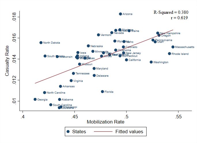
In today’s America, the typical woman has one or two children, is en-
gaged in paid work and enjoys the same legal rights as men. This has not
always been the case. At the end of the 19th century, approximately 5
percent of married white women were engaged in paid work and the total
fertility rate was about 3.5 (Goldin (1991); Guinnane (2011)). The de-
crease in fertility and the increase in female labor supply was not steady
and may have been shocked by specific events. For instance, fertility rates
declined from 1850 to 1930 and stabilized for several years. This stabiliza-
tion was followed by exceptionally high birth rates from 1944 to 1961–the
Baby Boom– and then a baby bust (Figure 1).1
    A vast literature documents historical shocks that could have led to
female economic empowerment in the 20th century (Fernández et al. (2004);
Fernández (2013); Fernández and Wong (2014a,b); Goldin (2006); Goldin
and Katz (2002); Guinnane (2011)). In this study, we reassess the role of
one of these potential shocks, World War II (WWII). During WWII, about
16 million men were mobilized and deployed in Asia and Europe, which
coincided with a sharp rise in female employment. At the height of the
war, women comprised approximately 35 percent of the civilian labor force
(Acemoglu et al. (2004)).
    Goldin and Olivetti (2013), Acemoglu et al. (2004) and Doepke et al.
(2015) rely on mobilization rates to identify the long run impact of the war
on female labor force participation, the wage structure and fertility, respec-
tively. Mobilization rates vary across states because of many factors (e.g.,
dependents, occupation and fitness to serve) that led to deferments. Using
this variation, Goldin and Olivetti (2013) provide evidence that women’s la-
bor supply was shifted during the war and that the effect persisted for some
of the women who worked in white-collar positions during WWII. Similarly,
Acemoglu et al. (2004) provide evidence that women worked more in 1950
in states with a higher mobilization rate and that this increase in female
labor supply lowered female and male wages. Doepke et al. (2015) find that
states with a greater mobilization of men experienced a larger post-war in-
crease in fertility. They argue that the return of men from the war crowded
out younger women leading them to opt for marriage and childbearing.
    Our purpose is to reexamine the effect of WWII on fertility and women’s
employment. We first investigate the reproducibility of the results de-
scribed above. We then complement these studies by relying on novel data
on male casualties at a more disaggregated level (i.e., county). Last, we
   1
    The increase in the female labor force participation was steady between 1930 to
1970.

                                        2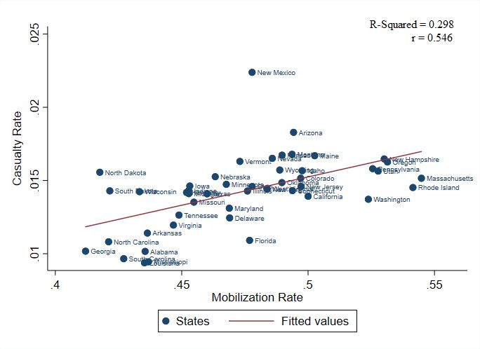
investigate some of the mechanisms through which WWII casualties may
have affected fertility, focusing on the labor and marriage markets.
We begin with a replication of Doepke et al. (2015)’s analyses using a
similar empirical model. We successfully replicate their main results and
show that state casualty and mobilization rates are positively correlated
to fertility post-WWII. One concern with their results is that socioeco-
nomic factors causing differences in male casualties or mobilization could
also affect post-war fertility. One key variable is race as the U.S. Army
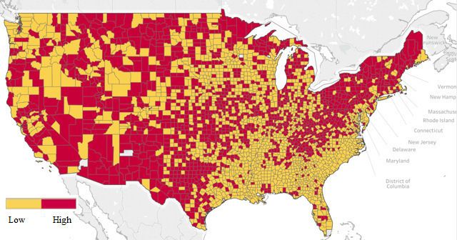
was still segregated when the U.S. entered WWII. Figure 2 illustrates the
geographic distribution of the casualty rates both across-states and within-
states, across-counties. This figure shows that the Deep South overwhelm-
ingly consisted of low-casualty rate counties, partly due to the U.S. military
segregation.2
We thus enrich Doepke et al. (2015)’s main specification with the share
of black men and additional control variables such as the share of fathers
and average educational attainment. Once we control for these additional
pre-war characteristics, the point estimates become negative, suggesting
that higher male causalities and mobilization rates led to lower fertility
post-WWII. This sensitivity analysis sheds light on the importance to fur-
ther control for key determinants of male mobilization (or casualty) and
fertility, and taking into account regional trends in fertility.3
We then turn to our novel county-level analysis. Our empirical strategy
consists of comparing counties with high and low casualty rates, before and
after the war. Analyzing the effect of WWII on fertility at the county-level
brings the analysis to a more disaggregated level. This has a key advantage
over the state-level analysis since counties across states may have very
different demographic and socioeconomic characteristics. Additionally, one
of the main sources of potential bias in cross-state regressions likely stems
from important regional trends in fertility. Relying on the county-level data
allows us to account for these trends by controlling for all time-varying state
characteristics and solely relying on the within-state variation. County-
level data thus strengthens the credibility of the identification strategy.
While most counties in the U.S. experienced a Baby Boom following
the war, we find that the increase in fertility was lower in high-casualty
2
When black men volunteered for duty or were drafted following the Pearl Harbor
attack, they were relegated to segregated divisions and combat support roles, such as
cook, quartermaster and grave-digging duty (Bristol and Stur (2002)).
3
Appendix Figure A1 shows that the U.S. South, in particular, had a unique fertility
trajectory. In the late 1940s, the gap between the South and other regions starts to
close, suggesting that regions with relatively higher casualty rate had a relatively lower
decrease in fertility.
3rate counties than in low-casualty rate counties in 1950. Our estimates are
statistically significant and suggest that women had, on average, about 15%
fewer babies in a county that had a one percentage point higher casualty
rate during WWII. We show that the sign of the county-level estimates is
robust to the inclusion of pre-war county determinants of WWII casualties,
as well as a set of extended controls that might have potentially affected
fertility levels. We also show that our findings are robust to the exclusion of
states with a large share of black residents or large post-war net migration.
Of note, we find weak evidence that WWII casualties affect fertility rates
in 1960 and no evidence that the war casualties impacted fertility in 1970.
In order to gain insight on the mechanisms through which WWII ca-
sualties may have decreased fertility, we follow the literature and test the
effect of male casualties on female employment and other socioeconomic
outcomes. We reexamine the effect of WWII on female employment at
the State Economic Area (SEA) level. A SEA is either a single county
or a group of counties. Our results are in line with those of Acemoglu
et al. (2004) and Goldin and Olivetti (2013) as we find that SEA-level ca-
sualty rates during WWII led to a shift in female employment in 1950. Our
findings also suggest that greater casualties reduced individual wages (Ace-
moglu et al. (2004)), but that the increase in after-war household income
was higher in high casualty rate SEAs than in low casualty rate SEAs.
This set of results suggests an explanation consistent with Becker’s the-
ory of fertility (Becker (1960); Becker and Lewis (1973); Becker and Barro
(1989)). Becker argued that parents derive utility from both the number
and the quality of children. When their earnings increase, parents tend
to be more likely to invest in their children’s human capital and decrease
the number of children they have. We provide empirical evidence sup-
porting this theory by relying on infant mortality data and computing the
percentage of live births attended by physicians at the hospital. We find
that county male casualties are positively associated to the percentage of
attended births by physicians at the hospital and negatively related to in-
fant mortality in the after-war period, indicating better health outcomes
for newborn kids. These results provide suggestive evidence that parents
in high casualty rate counties invest more in the quality of their children
during pregnancy and after birth.4
Another important channel through which male casualties could have
4
See Doepke et al. (2015) for a detailed account of the work of Becker on the quantity
and quality of children. Becker provides many examples of child quality choices such as
giving them dance and music lessons and sending them to private colleges.
4impacted fertility is male-to-female sex ratios and the marriage market.
A recent study by Brainerd (2017) shows that the drastic change in sex
ratios caused by World War II in Russia led to lower rates of marriage and
fertility and higher non-marital births, and reduced the bargaining power
within marriage for women in areas most affected by war casualties.5 Our
fertility results are in line with Brainerd (2017), but we find no evidence
that WWII casualties decreased marriage rates. This could be due to the
relatively small decrease in sex ratios for most U.S. counties (i.e., roughly
1%), compared to a decrease of about 28% in Russia. We also show that
WWII casualties led to a significant increase in the age of having a first
child for young women aged between 15 and 25 years old in 1950, which can
explain the decrease in fertility especially for women in this age category.
Overall, our analysis of the effect of WWII casualties on socioeconomic
outcomes provide plausible explanations for the negative relationship be-
tween male casualties and fertility in 1950. The absence of men during and
after WWII led to an increase in women’s employment during and after the
war, which increased household income. The combined effects of these two
phenomena slowed down the Baby Boom in counties with relatively more
casualties. Our findings thus suggest that there was a strong link between
young women’s labor market and fertility in the baby boom period, and
that the labor market was affected strongly by the war (Acemoglu et al.
(2004); Doepke et al. (2015)).
Our study contributes to a large literature providing socioeconomic ex-
planations to the Baby Boom.6 Previous studies have emphasized the role
of parents (Rutherdale (1999)), technological progress in the household
sector (Greenwood et al. (2005))7 , the Great Depression (Bellou and Car-
dia (2014)) and ideological and cultural changes (Lesthaeghe and Surkyn
(1988)). Albanesi and Olivetti (2014) also provide evidence that improve-
ments in maternal health contributed to the Baby Boom in the U.S. Using
cross-state variation, they show that the decline in maternal mortality is
associated with a rise in fertility for women born in the 1920–30s. Our
5
Abramitzky et al. (2011) evaluate the impact of war on assortative matching in the
marriage market and find that World War I has led to a decrease in the probability of
marriage for women in French regions with higher mortality rates.
6
One of the most well-known explanations for the Baby Boom is the “catch-up
fertility” hypothesis (Easterlin (1961)). This theory, based on the concept of “relative
income,” states that people who grew up during the Great Depression had low material
well-being and increased their demand for children during the post-WWII economic
expansion (Jones and Schoonbroodt (2016)).
7
Bailey and Collins (2011) provide empirical evidence that the Amish experienced a
Baby Boom and that appliance ownership and electrification are negatively correlated
to changes in fertility rate.
5county-level analysis allows us to control for this type of time-varying state-
level shocks.
Our paper also contributes to a literature that analyzes the effect of
war on fertility and female labor supply (Bellou and Cardia (2016); Beth-
mann and Kvasnicka (2013); Eder (2016); Boehnke and Gay (2017); Ja-
worski (2014); Vandenbroucke (2014)) and to a vast literature on sex ratios
and the marriage market (Carranza (2014); Grosjean and Khattar (2019);
Lafortune (2013); Qian (2008)).
We structure the remainder of the paper as follows. In section 1, we
present the data sources and descriptive statistics. Section 2 presents the
methodology. Section 3 replicates the results of Doepke et al. (2015) at the
state-level. In section 4, we provide the regression results for fertility at the
county-level and a large set of robustness checks. In the subsequent section,
we empirically examine the channels, and the last section concludes.
1 Data
1.1 World War II Casualties
During the war, 16 million Americans served in the United States Armed
Forces, of whom over 400,000 did not return home. Besides its random com-
ponent, the variation of male casualties across different counties is affected
by the occurrence of draft deferrals. The United States Armed Forces con-
sisted largely of “Citizen Soldiers” drawn from civilian life. The majority,
roughly 10 million, joined the military through the draft, and most draftees
were assigned to the army. However, the Selective Service granted defer-
ments based on specific factors such as marital status, fatherhood, combat
skills including the ability to serve, and medical disabilities. Mobilization
rates for fathers were low as they were generally drafted last in the local
draft pool. Furthermore, deferments were offered based on occupation. One
of the main determinants of draft deferments was farmer status as farming
was needed to maintain the level of food supply during the war. Note that
most deferments were eliminated during the war. For example, both the
wife and child deferment ended in 1943 (Goldin and Olivetti (2013)).
We rely on monographs from the National Archives to construct our
measure of military casualties at the county-level. The dataset is compiled
by the Department of the Navy and Bureau of Naval Personnel using The
Honor List of Dead and Missing for each state in the United States, pub-
lished by the War Department. This list contains the most complete data
available on all military personnel who were killed up until January 31,
61946. Errors in this list were minimized by careful checks by the Casualty
Branch of The Adjutant General’s Office and by Machine Records Units.
Note that civilian casualties are not included in these reports.
We construct casualty rates at the county-level as the number of men
killed in action during WWII, divided by the number of men between the
ages of 18 and 44 in 1940, and multiplied by 100. Census data on male
population in 1940 per age category is retrieved from the National Historical
Geographic Information System (NHGIS). Note that the 1940 Selective
Service and Training Act required that men between the ages of 21 and
35 register to the draft. Registration was extended a few times during the
war, including a new Service Act which made men between 18 and 45 liable
for military service. By the end of the war in 1945, 50 million men between
18 and 45 had registered for the draft and 10 million had been inducted in
the military. We thus rely on the male population of this age group as a
proxy for the number of registered men (Acemoglu et al. (2004)).
1.2 Fertility and Socioeconomic Characteristics
Our analysis uses fertility and socioeconomic characteristics of women and
children before and after WWII as the primary outcomes of interest. Data
on fertility is from the 1915–2007 U.S. County-Level Natality and Mortality
Data (Bailey et al. (2016)), retrieved from ICPSR. We rely on the number
of total live birth by place of occurrence between 1933 and 1972. Note that
data on births by place of occurrence begins to be complete in the dataset
starting 1933. Additionally, total births at the county-level are available
for the years 1915–1941 from Vital Statistics: Natality & Mortality Data.
For the female population, we only consider women of childbearing age
(i.e., between 15 and 44 years old) for the years 1915–1972 also from Vital
Statistics: Natality & Mortality Data. 8
For data on the number of children, labor supply, age of first time
mothers, personal earnings, and other individual characteristics, we rely on
Census data from the 1% Integrated Public Use Microdata Series (IPUMS)
of the 1940 and 1950 censuses (Ruggles et al. (2010)). Unfortunately, this
dataset is not available at the county-level for 1950. We thus rely on data at
the SEA-level for this analysis. SEA stands for State Economic Area (see
8
Total births and population data are from the Census Bureau’s vital statistics
annual reports for states (including territories) and counties. Births are limited in geo-
graphic extent to the Birth Registration Areas established in each year. Michael Haines
at Colgate University provided NHGIS with the source data, which were entered from
printed census publications, and NHGIS researchers organized the data into tables and
assigned meta-data on topics, categories, etc.
7Bogue (1951) for more details). An SEA is either a single county or a group
of counties within the same state that have similar economic characteristics.
Importantly, the definitions of SEAs in 1940 and 1950 are similar. The age
of a first time mother is computed by subtracting the age of the eldest child
from the age of the mother. To measure labor supply, we use a dummy that
indicates whether a woman is currently employed, and the total number of
weeks worked per year. Personal earnings are considered for employed men
and women, and are deflated by the 1990 CPI.
To examine the impact of WWII casualties on infants’ health, we rely on
the percentage of live births attended by physicians at hospital and infant
mortality measured as the death of young children under the age of one.
County-level data on births by attendant by place of residence is available
between 1939 and 1959 from NHGIS, derived from annual reports of vital
statistics for states (including territories) and counties from the U.S. Census
Bureau (1939–1944) and the U.S. Public Health Service (1945–1959). For
infant mortality, data is available by place of occurrence from 1915 to 1941,
and from 1959 to 1972 originally from Vital Statistics: Natality & Mortality
Data.9
1.3 Descriptive Statistics
Table 1 displays summary statistics for WWII casualties, fertility and fe-
male population by decade for 1940–1970. The average number of casualties
by county is about 99. The standard deviation is remarkably large (422)
at the county-level. As mentioned previously, the casualty rate is the frac-
tion of registered men who were killed during World War II. The casualty
rate is roughly 1 percent and the standard deviation is 0.39. We split the
sample into low-casualty and high-casualty counties using the casualty rate
mean. There are a total of 3,070 counties, 1,639 of which are in the low
casualty rate category. The mean casualty rate for low- and high- casualty
rate counties is 0.78 and 1.26 percent, respectively.
The average number of total live births per county increased by approx-
imately 50% between 1940 and 1950, illustrating the Baby Boom period.
This increase occurred in both high and low casualty rate counties, al-
though the increase was larger in low casualty rate counties for 1950 and
1960.
9
The 1959–1967 data are derived from printed annual reports from the U.S. Public
Health Service. The 1968–1972 data are derived from individual-level microdata (either
birth certificates or the Compressed Mortality File) from the National Center for Health
Statistics.
8Appendix Table A1 reports means and standard deviations for the in-
dividual characteristics of interest at the SEA-level. The average age of
mothers at the time of first birth, women’s employment rate and weekly
wages all increased after the war. Of note, women’s employment rate in-
creased from 25% in 1940 to 31% in 1950. This increase was larger in high
casualty rate counties.
2 Identification Strategy
In this section, we first show that casualty and mobilization rates are highly
correlated. We then discuss the identification assumption and describe the
main specification
2.1 State Casualty and Mobilization Rates
Male mobilization during the war might be seen as the best source of ex-
ogenous variation across states or counties.10 However, to the best of our
knowledge, data on male mobilization at the county-level is unavailable.
Instead, we rely on male casualties as a measure of WWII intensity for our
county-level exercise. Our analysis thus differs from Acemoglu et al. (2004),
Doepke et al. (2015) and Goldin and Olivetti (2013) along two dimensions.
First, we rely on novel county-level data instead of state-level data. This
means that we are exploiting within-state across-county variation instead
of across-state variation. Second, our identifying variation comes from ca-
sualty rates instead of mobilization rates. We provide empirical evidence
throughout that the latter dimension does not drive our main conclusions.
Figure 3 illustrates that differences in casualty rates mostly reflect differ-
ences in mobilization rates. This figure plots both state mobilization and
casualty rates. Male casualties are positively and highly correlated with
male mobilization at the state-level. The correlation coefficient between
mobilization and casualty rates is 0.55.11
10
According to the National WWII Museum, 61.2% of the military were drafted,
while only 38.8% were volunteers.
11
New Mexico faced the highest rate of casualties, exceeding 350 per 100,000 people
during WWII, and possibly represents an outlier. Excluding New Mexico makes the
positive relationship between male mobilization and casualties stronger, with a correla-
tion coefficient of 0.62 (see Figure 3, second panel). Excluding New Mexico from the
analysis has no effect on our conclusions. Results available upon request.
92.2 Identification Assumption
This paper relies on the parallel trends assumption that in the absence of
male war casualties, the average change in birth rates would have not been
systematically different between counties with low- and high-casualty rates.
This identification assumption could be violated if the casualty rate is re-
lated to pre-war demographic and socioeconomic characteristics of counties.
We argue in what follows that our results are not driven by pre-war factors.
As shown in Table 1, the number of casualties was not uniform across
counties. As with mobilization rates, the variation in the cross-county
casualty rates could arise from observable economic factors in addition to
the random component. Our concern is that socioeconomic factors causing
differences in male casualties also affect our outcome variables.
Race The United States military was still segregated during World War
II. Even though mobilized men were randomly drafted from the registered
pool, less than 4,000 African-Americans were serving in the military and
only 12 African-Americans were officers in 1941. In fact, during the war
period, the segregation practices of civilian life spilled over into the military.
Pressures from the National Association for the Advancement of Colored
People led President Roosevelt to pledge that African-Americans would be
enlisted according to their percentage in the population.12 Although this
percentage was never actually met during the war, the number of African-
Americans in the army grew drastically. Of note, though, blacks were often
classified in separate units for combat and were not allowed to fight on the
front lines. They were mostly given support duties and were not allowed
to be in units with white soldiers. A total of 1.2 million African Americans
served in the U.S. Armed Forces in segregated divisions and 708 were killed
in action.13 Below, we show that our main findings are robust to excluding
states with a high black population from the analysis.
Education In addition to fitness, the selection of men to serve in the army
may have been related to education. Between June and July 1943, 8% of
white troops rejected and 34.5% of African-American troops rejected were
for educational deficiencies (Jenkins et al. (1944)). Men were tested and
12
It was not until 1948 that President Harry S. Truman ordered a desegregation of the
Armed Services and equality of treatment and opportunity in the U.S. military without
regard to race, color, religion or national origin.
13
By the end of war, it became more acceptable to have integrated units of both
black and white soldiers fighting side by side on the front line in order to maintain the
strength of the military (see Sandler (1992) and Wynn (1993)).
10sent to units based on their educational backgrounds. For instance, ser-
vicemen in the infantry branch were less educated as the infantry required
a lower logistical burden. Infantry soldiers (also known as foot soldiers)
operated under the worst conditions and performed missions that were not
assigned to any other units. Even though the infantry branch faced the
highest number of casualties, it constituted only 6% of the entire units.
Additionally, Appendix Figure A2 shows a weak positive correlation be-
tween casualty rates and the county’s average years of education for men
between 18 and 44 years old in 1940.
Economic Conditions One of the main reasons for deferment was farm
occupation in order to maintain the food supply during the WWII period.
Acemoglu et al. (2004) show that there is a negative correlation between
male mobilization and a state’s percentage of farmers. With male farmers
being deferred, we would expect fewer casualties in rural counties. Addi-
tionally, deferments of drafted men could potentially be affected by their
economic conditions. Wealthy and connected men could avoid being mo-
bilized or get assigned to non-combat roles. For example, poor men who
did not have a record of private medical care may find it harder to obtain
medical deferments. However, Appendix Figure A3 shows that the casualty
rate and the county’s average wage income of men aged between 18 and 44
in 1940 are very weakly correlated.
As a robustness check, we will include the covariates identified by Ace-
moglu et al. (2004) to our baseline model to account for correlates of differ-
ences in casualty rates by county that may affect our main outcome. Our
results are robust to including 1940 county specific characteristics (such
as fathers share, black population share, and average years of education)
interacted with the after war year dummies, which suggests that our identi-
fication assumption is credible. Additionally, we include county fixed effects
in the empirical analysis to control for any county specific time-invariant
characteristics that may affect fertility.
2.3 Model Specification
Our hypothesis is that the increase in fertility during the Baby Boom period
was lower in counties where World War II casualty rates were high. To
investigate this hypothesis, we estimate the following specification:
yct = λc + δdwar + µdwar × Rc + Xct′ ω + εct (1)
11where yct is the natural log of total live births or birth rates in county c
and year t. We include a full set of county dummies λc to control for time-
invariant county characteristics. The variable dwar equals one for after-war
years and zero for the pre-war period. The after war dummy takes the
value of zero for 1940 and one for the years 1950, 1960, and 1970 in different
regressions, each of which includes data for 1940 and one of these years.
This allows us to investigate the short run and the long run effects of war
casualties on fertility. The variable Rc is the casualty rate by county. In
the binary regressions, it takes the value of one if the county belongs to the
high casualty rate category and zero if the county is in the low casualty
rate category. In the continuous regressions, this variable is defined as
continuous to estimate the impact of a percentage point increase in the
casualty rate on fertility. The interaction of dwar and Rc shows the effect
of the treatment. The coefficient of interest here is thus µ. We cluster
standard errors at the county-level.
Xct is a vector of covariates including the natural log of female popu-
lation of childbearing age (i.e., between 15 and 44 years old). Using the
general fertility rate computed as the number of live births by 100 women
as the dependent variable yields similar findings (see section 4).
In section 3, we rely on the state-level variation of these variables in
order to reconcile our county-level findings with previous studies at the
state level.
As a robustness check, we include state-decade fixed effects to relax the
identification assumption. The inclusion of state-decade fixed effects in the
model allows us to control for time-varying state policies and shocks such as
cross-state variation in pregnancy-related mortality (Albanesi and Olivetti
(2014)).
In a set of robustness checks, we control for pre-war county’s demo-
graphic and socioeconomic characteristics. This is an important specifica-
tion check since these factors may have caused differences in casualties and
fertility and thus lead to a bias in our estimates. More precisely, we interact
the “After War” dummy with the following socioeconomic characteristics
to allow them to differ by decade: the share of male farmers between the
ages of 18 and 44, the share of black men between the ages of 18 and 44,
the share of fathers between the ages of 18 and 44 and the average years
of education for men between the ages of 18 and 44. We also control for
county-level lagged changes between census years 1930–1940 (interacted
with the “After War” dummy) in economic or demographic variables that
could affect fertility such as Age at First Marriage (for married women
12only), Dwelling Ownership (share of those who own a dwelling out of to-
tal population for both men and women above the age of 16), and Female
Labor Force Participation (for women aged between 16 and 64).
3 State-Level Results
Before turning our attention to our novel county-level male casualty data,
we first replicate the results of Doepke et al. (2015) at the state-level. This
exercise serves at least two purposes. First, we believe reproducibility is
a key part of the scientific method, and that replications may help to im-
prove our understanding of previous research findings. Second, this exercise
may shed some light on the key differences between our state and county
analyses.
We first replicate the findings of Doepke et al. (2015) using a similar
specification. We then explore the robustness of their results to additional
control variables. Our replicated results are presented in Table 2, which
contains OLS estimates of equation 1 at the state-level. In their analysis,
Doepke et al. (2015) rely on pooled census data from 1940 and 1960 and
restrict the sample to women aged between 25 and 35 years old.14 Their
main dependent variables are “Children under age of 5” and “Children ever
born”. For our replication, we rely on the number of children under the
age of 5 (columns 1–4) from the pooled micro data from the 1940 and
1960 censuses and complement this analysis using data on the number of
total live births (columns 5–8) from Vital Statistics. In the top panel, we
rely on the casualty rate, while the bottom panel shows estimates for the
mobilization rate. Columns 1, 2, 5 and 6 present estimates for the binary
regressions, in which the casualty (or mobilization) rate variable is a dummy
that takes the value of one for high-casualty (or mobilization) rate states
and zero for low-casualty (or mobilization) rate states. Columns 3, 4, 7
and 8 show estimates for the continuous regressions, in which casualty (or
mobilization) rate is a continuous variable.
We successfully replicate the state-level results in Doepke et al. (2015)
using both mobilization and casualty rates. In columns 1 and 3, we find
that state casualty and mobilization rates are positively correlated with
the number of children under the age of 5 for women aged between 25
and 35 years old. The point estimates are strikingly similar in the binary
form regressions but differ in magnitude in the continuous form ones. The
14
The authors distinguish between two age groups, women aged 25 to 35 defined as
“young” and women aged 45 to 55 defined as “old”. We focus on the younger group of
women on which the effect of WWII mobilized men is documented.
13large difference in magnitudes is due to differences in means as the mean
for the casualty rate is around 1%, while the mean for the mobilization
rate is around 45%. For instance, Beta coefficients suggest that a one
standard deviation increase in casualty rates leads to an increase of 0.03
standard deviation in total births, while a one standard deviation increase
in mobilization rates is associated with a 0.04 standard deviation in births
(column 3).
We confirm these results from Census data by relying on total births
count from Vital Statistics data. In columns 5 and 7, the point estimates
for the binary form regressions are positive and statistically insignificant
(and of similar magnitude) for both mobilization and casualty rates. The
point estimates for the continuous form are also positive, but significant
only for mobilization. Overall, these results suggest that Doepke et al.
(2015)’s main results are reproducible and that relying on casualty rather
than mobilization leads to similar conclusions.
To further examine the reproducibility of Doepke et al. (2015)’s conclu-
sions, we add pre-war state demographic and socioeconomic characteristics
to the model. More precisely, we add a set of controls to account for state
characteristics that may have caused differences in casualties and mobiliza-
tion: the share of male farmers between the ages of 18 and 44, the share of
black men between the ages of 18 and 44, the share of fathers between the
ages of 18 and 44 and the average years of education for men between the
ages of 18 and 44. All controls are interacted with the “After War” dummy
to allow them to differ by decade. The point estimates are presented in
columns 2, 4, 6 and 8. We also conduct validation tests for unobservable
selection and coefficient stability in columns 2, 4, 6, and 8 following Oster
(2019)’s methodology.15
Conditional on these controls, the estimates at the state-level for casu-
alty and mobilization rates become negative, suggesting an omitted variable
bias in the state-level estimates. In other words, the estimates for the bi-
nary and continuous form regressions for both mobilization and casualty
rates have a negative sign once we control for selected pre-war state char-
acteristics. Among the included pre-war characteristics, the share of black
men is the key variable causing the switch in sign.
These findings provide a major motivation to the use of a finer geo-
graphic level for analyzing the impact of WWII casualty on fertility since
15
Oster (2019) argues that |δ|>1 leaves a limited scope for unobservables to explain
the results. Our reported parameter δ thus suggests that the controlled variables are
important counfounders to the relationship between missing men and fertility.
14states may be composed of counties with very different socioeconomic char-
acteristics and with different casualty and fertility rates. In section 4, we
show that the sign of our county-level estimates is robust to the inclu-
sion of a large set of pre-war county characteristics, as well as state-decade
dummies.
To sum up, we successfully replicate Doepke et al. (2015)’s fertility re-
sults using similar specifications, but provide evidence that the estimates
are not robust to the inclusion of key pre-war state characteristics. We
argue that relying on county-level data strengthens the credibility of the
analysis as it provides the possibility to further control for other (poten-
tially) important state-shocks and state-decade fixed effects. Of note, we
have shown that the choice of data source (vital statistics versus pooled
Census data) and treatment measure for the intensity of war (mobilization
versus casualty rate) does not affect our state-level conclusions.
4 County-Level Results
In this section, we estimate the treatment effect of war on fertility by using
male casualty rates as a measure of war intensity. Our analysis is now at
the county-level and our model includes county fixed effects.
4.1 Impacts on Fertility
Table 3 contains OLS estimates of equation 1. The dependent variable is
the natural log of total live births. We cluster standard errors at the county-
level. We include county fixed effects and control for the female population
in all the regressions. Columns 1, 3 and 5 present estimates for the binary
regressions, in which the casualty rate variable is a dummy that takes the
value of one for high-casualty rate counties and zero for low-casualty rate
counties. Columns 2, 4 and 6 show estimates for the continuous regressions,
in which casualty rate is a continuous variable.
What clearly emerges is that county casualty rates are negatively asso-
ciated with total live births in 1950. Columns 1 and 2 show the estimates
for the years 1940–1950. Results indicate that there was a large and highly
significant difference in the fertility change between high- and low- casualty
rate counties over this time period. The estimate in the binary regression is
negative and statistically significant at the 1% level, suggesting that high-
casualty rate counties had significantly fewer total live births compared to
counties with lower casualty rates. Interestingly, the increase in the total
live birth in 1950 seems to be offset by WWII casualties in the high ca-
15sualty rate counties. In the continuous regression, the point estimate of
-0.166 (standard error of 0.04) implies that a one percentage point increase
in the male casualty rate during World War II leads to a 15.3% decrease in
fertility.
Columns 3 and 4 show comparable estimates for the years 1940–1960.
There is weak evidence that WWII casualties affected total live births in
1960. While the coefficient of the binary regression becomes statistically
insignificant, the estimate in the continuous regression shows a persistent
effect of male war casualties. Columns 5 and 6 suggest that WWII casu-
alties did not affect fertility rates in 1970. The estimates are statistically
insignificant and smaller in magnitude than for columns 1–4. This result
is not surprising as many women of childbearing age (in 1970) were born
after WWII.
To observe how the gaps in fertility have been opening and closing
during the pre- and post-war period, we rely on yearly county-level data on
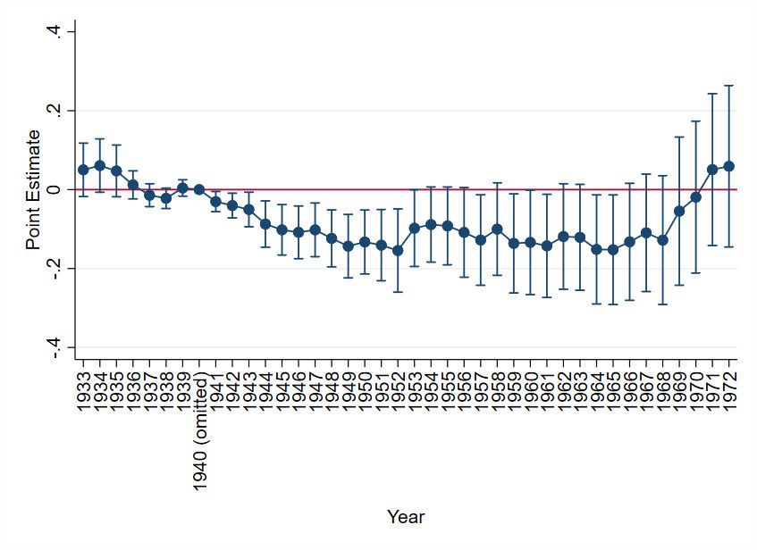
births by place of occurrence from 1933 to 1972. We illustrate our results
by plotting the estimated coefficients from the continuous regression on the
natural log of total live births in Figure 4. We omit the year before the
entry of the U.S. into WWII, i.e., 1940 is the reference year. We confirm the
pre-treatment trends in the period between 1935 and 1939 and a temporary
negative effect of war male casualties on total live births during the 1950s
and 1960s, with the impact completely fading away during the early 1970s.
Of note, the negative effect starts as early as 1941, when the U.S. was not
at war. This result is consistent with increased mobilization activity at the
time, even in 1940–1941 in advance of U.S. entry into the war. According
to the US Army Center of Military History, mobilization evolved from its
gradual beginnings in 1940, speeding up in 1941, expanding dramatically
in 1942, and reaching its peak in production in 1943. With the German
invasion of Poland in September 1939, President Roosevelt proclaimed a
limited national emergency and authorized an increase to 227,000 for the
Regular Army and to 235,000 for the National Guard. Thus, a sizeable
number of men were employed in the army before the U.S. officially entered
the war in December 1941.
We check in Table 4 whether our findings are driven by time-varying
changes at the state-level. Our analysis relies on within-state across-county
variation because we control for state-decade fixed effects in our model. The
inclusion of state-decade fixed effects has no effect on our main conclu-
sions. Our estimates remain negative and statistically significant, although
smaller in magnitude.
16In Appendix Table A2, columns 1–2, we test the parallel trend as-
sumption by looking for pre-trends. This assumption requires that in the
absence of WWII casualties, the difference between high and low casualty
rate counties has a constant trend over time. Unfortunately, county data
on total live births are not available for 1930. We instead have to rely
on total births. Our pre-war estimates indicate that there was no signif-
icant relationship between the change in total births from 1930 to 1940
and county casualty rates during WWII. The estimates for both the binary
and continuous regressions are very small and statistically insignificant at
conventional levels.
So far, our results provide suggestive evidence that war casualties had
a negative effect on fertility. In other words, male casualties during WWII
may have slowed down the rise of fertility for counties with many war
casualties. We check the robustness of our results in the next subsection.
4.2 Robustness Checks
In a first set of robustness checks, we examine the endogeneity of our main
independent variable by regressing the natural log of total live births in
1940 on the casualty rate at the county-level. Appendix Figure A4 shows
that the regression coefficient is equal to zero, suggesting that casualty rates
do not explain the pre-war levels of total live births across counties.
In another set of specification checks, we replicate our analysis of Table
3, but controlling for pre-war county demographic and socioeconomic char-
acteristics, in Appendix Table A3. As mentioned in Section 2, we interact
the “After War” dummy with socioeconomic characteristics to allow them
to differ by decade. We also control for county-level lagged economic and
demographic changes between census years 1930–1940 (interacted with the
“After War” dummy).16 Moreover, due to the endogeneity of the farmers’
share, we drop counties with higher than 80% share of male farmers (aged
between 18 and 44) in 1940. Our point estimates for 1950 and 1960 are
smaller in magnitude, but remain statistically significant at conventional
levels. In contrast, our point estimates for 1970 are now larger and signifi-
cant for the continuous regression.17
In Appendix Table A5, we add the set of covariates to the specification
including state-decade fixed effects. The point estimates are similar to
16
The inclusion of the extended set of controls in the state-level analysis of Table 2
does not affect our findings. See Appendix Table A4.
17
While the reported Oster (2019) test highlights the potential importance of unob-
served confounders in the baseline models, the additional covariates have limited influ-
ence on the estimates as the pattern of our findings remains unchanged.
17Table 4 and Appendix Table A3, suggesting that the inclusion of state
trends or demographic characteristics equally affect the magnitude of our
estimates.
We also check whether the negative relationship between fertility and
WWII casualties is driven by less populous counties. To rule out this
idea, we split the sample by the median share of counties’ population in
1940 relative to the state’s population to which they belong in Appendix
Table A6. The estimates for the binary (continuous) regressions are larger
(smaller) in magnitude in less populous counties in 1950 and 1960. As
as additional exercise, we also weight counties by this population share in
Appendix Table A7.18 The estimates remain negative and significant. The
estimates for the binary regressions are smaller in magnitude for 1950 and
1960, while the estimates for the continuous regressions are larger than in
our baseline.
We also show that the negative effect of WWII casualties on births oc-
curred in both rural and urban counties. In Appendix Table A9, we split
the sample into two groups of counties based on the share of urban popu-
lation in 1940, i.e., above and below the median. The estimates for 1950
and 1960 are negative and of similar magnitude for both set of counties.
Overall, our findings suggest that the negative impact of war casualties on
fertility at the county-level is not solely driven by less populous (or rural)
counties.
In our main specification, we are controlling for female population. This
may be an issue if female population was affected by WWII. Instead of the
raw birth counts, we examine the impact of WWII male casualties on birth
rates computed as the number of total live births divided by the female
population aged between 15 and 44, and multiplied by 100 for each county
and decade. Our estimates are presented in Appendix Table A10.19 Our
main findings remain mostly unchanged and suggest that casualty rates are
negatively related to fertility in 1950 and 1960.
To provide a check of whether our findings are driven by states with a
large share of black residents, we replicate our baseline analysis, but exclude
states where the population is more than 20% black. The estimates are
presented in Appendix Table A12. Our estimates are slightly smaller in
magnitude, but have the same sign and remain statistically significant at
conventional levels.
18
Weighting counties based on their 1940’s population relative to the 1940 U.S. pop-
ulation yields similar results (see Appendix Table A8).
19
Our results are also robust to controlling for the total population instead of the
female population. Appendix Table A11 shows the estimates.
18Last, to better understand the distribution of our main independent
variable, we illustrate the variation in casualty rates across counties in
Appendix Figure A5. The casualty rates’ distribution is symmetric and
unimodal. Therefore, splitting casualty rates across groups at the median
rather than the mean does not affect our main results. (See Appendix Table
A13 for the analysis.) The figure also shows a right tail to the distribution
suggesting the presence of outliers for the top values of casualty rate. As
this might affect our findings when relying on this variable in its continuous
form, we exclude the top 1% of casualty rate counties (i.e., 30 counties with
casualty rate above 2.11) in Appendix Table A14. Our results in 1950 hold
and become larger in magnitude for the continuous form, while the estimate
from the 1960 continuous regression slightly decreases in magnitude and
loses its significance. Our estimates in columns 5 and 6 are insignificant
and approximatively equal to 0, confirming the absence of the effect in
1970.
4.3 Migration
We now turn to analysing the role of selective migration after the war.
Arguably, men residing in counties with relatively fewer casualties might
migrate to counties where sex ratios are more imbalanced. There are plau-
sibly better job opportunities in high casualty rate counties and relatively
more unmarried women. In other words, geographical differences in the
thickness of the job and marriage markets due to the war could lead to se-
lective migration. Selective migration would “compensate” for missing men
in high casualty rate counties. We would thus be underestimating the effect
of WWII casualties in our baseline analysis. To examine whether our re-
sults are driven by selective migration, we repeat our baseline analysis, but
exclude counties with very negative and very positive net migration after
the war. More precisely, we exclude counties that are below and above one
standard deviation from the mean in total net migration, i.e., we restrict
the sample to counties in a bandwidth of total net migration between -30
and 10 net migrants per 100 individuals.
Appendix Table A15 presents our estimates for this subset of counties.
This table has the same structure as Table 3. The coefficients of interest
in columns 1, 3 and 5 are virtually identical to the ones in Table 3, while
the estimates for the continuous regressions for the years 1950 and 1960
(columns 2 and 4) are larger in magnitude.
195 Channels
Our findings so far are intriguing because WWII casualties are negatively
correlated to fertility during the 1950s relative to before the war. In this
section, we discuss different mechanisms through which male casualties
could have impacted fertility. We then rely on data at the SEA-level to
test some of these channels.
5.1 Fertility
Before turning our attention to the mechanisms, we check whether our fer-
tility results are similar at the SEA-level. Appendix Table A16 provides
summary statistics. There is a total of 466 SEAs, 243 of which are catego-
rized as high-casualty rate.
Appendix Table A17 presents estimates of equation 1 where the de-
pendent variable is the natural log of total live births. The structure of
the table is the same as Table 3. The only differences are that we replace
our county fixed effects by SEA fixed effects, and that the standard errors
are now clustered at the SEA-level. Our estimates and conclusions are
very similar. The estimates are all negative and statistically significant in
columns 1–4. The estimated effect remains negative and not statistically
significant in 1970, with a smaller magnitude. Of note, estimates from the
SEA-level binary measures are not directly comparable to the county-level
measures due to the difference in means between groups. Our rescaled co-
efficient estimate in column 1 suggests that high-casualty rate SEAs had
around 8% fewer total live births compared to those with lower casualty
rates, which is close in magnitude to our county-level findings.
5.2 Mechanisms
The absence of men during WWII could have led to a slowdown in the
fertility increase during the Baby Boom period through many channels.
A first mechanism through which WWII casualties may affect fertility is
the increase in female employment. During WWII, women across the U.S.
were highly encouraged to work in different industries and take over jobs
previously done by men. “Rosie the Riveter”, a cultural icon of WWII, is
now used as a symbol of American feminism and women’s economic power.
Acemoglu et al. (2004) document that the war induced a large positive
shock to the demand for female labor as male mobilization drew many
women into the workforce permanently. While men were fighting the war,
20millions of women were drawn into the labor force and replaced men in
factories and offices. In the same line, Goldin and Olivetti (2013) provide
empirical evidence that married women without children experienced the
largest increase in labor force participation and weeks worked.
An increase in the female employment both during and after WWII
would potentially lead to a decrease in fertility rates due to an increase in
the cost of having and raising a child. In high casualty rate counties, the
higher share of women who work have less time to raise children, and thus
may decide to have fewer children.20
In the “quality-quantity” trade-off theory proposed by Becker (1960),21
increases in wages induce parents to substitute the quantity of children for
higher quality. Despite the fact that Acemoglu et al. (2004) found that the
shift in female labor force participation increased market competition and
lowered individual wages, the existence of an additional source of income
within a household would have a positive impact on the couple’s earnings.
An increase in household wages could tempt married couples to favor qual-
ity of children over quantity.22
5.3 Quality-Quantity Trade-Off
We now test whether WWII casualties affected female employment and
household income using individual-level data. An increase in household
income could lead parents to substitute the quantity of children for higher
quality. The econometric model is as follows:
′
yist = λs + αdwar + βdwar × Rs + Xist γ + εist , (2)
where yist is the outcome variable of interest for individual i from SEA s
in year t. Rs is the casualty rate by SEA, while dwar equals one in 1950
(post-WWII) and zero in 1940 (pre-WWII). The interaction of dwar and
Rss shows the effect of WWII casualties on the outcome variable. β is thus
20
A recent study by Vandenbroucke (2014) builds and calibrates a fertility model to
fit the birth rate in France from 1800 until World War I (WWI). He finds that the fall
in the birth rate during the war is mostly due to the loss of expected income associated
with the risk that a wife remains alone. Boehnke and Gay (2017) also provide evidence
that areas with relatively more military casualties in France during WWI experienced a
larger increase in female labor throughout the interwar period.
21
A vast literature focuses on this channel. See Becker and Barro (1988), Becker and
Barro (1989), Galor and Weil (2000), Jones et al. (2011), Albanesi and Olivetti (2014),
Manuelli and Seshadri (2009), and Vandenbroucke (2014).
22
Higher incomes could also facilitate the adoption of modern household technologies
(Bose et al. (2020)). Access to modern household technologies would free women’s time
from basic housework, which may have led to increased investments in children’s health
(Lewis (2018)).
21our coefficient of interest. Xist is a set of individual characteristics. Our set
of (exogenous) individual characteristics includes age, race and ethnicity.
We also include the following (potentially endogenous) controls in some
specifications: marital status, education and experience. We include SEA
fixed effects and report standard errors clustered at the SEA-level.
Table 5 displays the results of this model. Each entry shows the estimate
of the interaction term coefficient β for a different specification. Columns 1–
3 (4–6) present estimates for the binary (continuous) regressions. Columns
1 and 4 only include SEA fixed effects. In columns 2 and 5, we add to
the model our set of exogenous controls. Columns 3 and 6 also control for
marital status, education level and experience of the individual.
The first and second panels show the effect of WWII casualties on female
employment and weeks worked per year for women of childbearing age. The
estimates are statistically significant at the 1% level and suggest that female
employment and weeks worked were higher in SEAs with higher casualty
rates. The point estimates suggest that female employment in 1950 was
1.1 percentage points higher, and that women of childbearing age worked
an additional 1.4 weeks per year, in high casualty rate SEAs. Controlling
for age, race and ethnicity does not change the size or significance of the
estimates.
These findings provide suggestive evidence that women living in areas
with more male casualties were more likely to stay in the labor market (and
work more weeks) after the war.23 These findings are in line with the idea
that decreased fertility in high-casualty rate counties is partly due to the
induced shifts in female labor supply during and after WWII.
The third and fourth panels test whether the SEA casualty rate is re-
lated to wages and household income. Acemoglu et al. (2004) show that
women worked more after the war in states with higher mobilization rates,
which lowered female and male wages. Our estimates support their find-
ings, showing that weekly wages for males and females working for at least
35 hours per week were lower in areas where the casualty rate was high.24
However, we think it is more relevant to look at the effect of war casualties
on the household’s income as it relates directly to Becker’s quality-quantity
23
It has not been clearly established why so many women stayed in the labor market
after the war. Acemoglu et al. (2004) hypothesize that it is possibly due to a change
in women’s preferences, opportunities and/or information about available work. See
Mulligan (1998) for an investigation of the causes of the increase in female labor force
participation during WWII.
24
The sample is restricted to individuals between the age of 15 and 65. Top-coded
values are imputed as 1.5 times the censored value. Farmers, self-employed and unpaid
family workers are excluded.
22You can also read