WP 4: Multi-level modelling of Land Use and population dynamics - Smartpop Project

Distribution: General

Final report

WP 4:
Multi-level modelling of Land Use and population
dynamics
Poelmans Lien, Uljee Inge, Van der Meulen Maarten, Verachtert Els, Lauwaet Dirk, Hallot Eric (ISSeP)

Study accomplished under the authority of
Belspo – Stereo III

November 2018

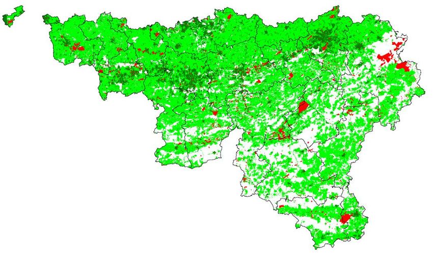
Table of Contents

All rights, amongst which the copyright, on the materials described in this document rest with the Flemish Institute for Technological Research NV
(“VITO”), Boeretang 200, BE-2400 Mol, Register of Legal Entities VAT BE 0244.195.916.
The information provided in this document is confidential information of VITO. This document may not be reproduced or brought into circulation
without the prior written consent of VITO. Without prior permission in writing from VITO this document may not be used, in whole or in part, for the
lodging of claims, for conducting proceedings, for publicity and/or for the benefit or acquisition in a more general sense.

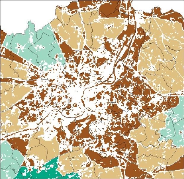
Table of Contents

TABLE OF CONTENTS

Table of Contents ________________________________________________________________ I

List of Figures __________________________________________________________________ III

List of Tables ___________________________________________________________________ VI

CHAPTER 1 Background and Objectives ____________________________________________ 7

CHAPTER 2 General modelling concept ____________________________________________ 8

CHAPTER 3 Application of the ACA land-use model in the Walloon region _______________ 12
 3.1. Global level: demand for activity and demand for land 12
 3.1.2. area demands in Business-as-Usual scenario ______________________________ 13
 3.1.3. Area demands in the Stop au béton scenario ______________________________ 17
 3.1.4. Area demands for land-use types, not associated with activities_______________ 18
 3.2. local level 18
 3.2.1. Land uses __________________________________________________________ 19
 3.3. Activity maps 21
 3.4. Suitability 21
 3.5. Zoning 24
 3.6. Accessibility 27

CHAPTER 4 results: Land use change in the Walloon region towards 2050 _______________ 30
 4.1. Land use change in the Walloon region towards 2050 30
 4.2. General trends in the Walloon region compared to Flanders 33
 4.3. Population densities 34

CHAPTER 5 Results: extra spatial indicators ________________________________________ 37
 5.1. Urban typology 37
 5.2. Degree of urbanisation 39
 5.3. Cluster size of built-up areas 40
 5.4. Cluster size of open space 42
 5.5. Distance to railway stations 43
 5.6. Urban pressure on agricultural land 45
 5.7. Urban Heat Island effect 46

CHAPTER 6 Conclusions ________________________________________________________ 55

References ____________________________________________________________________ 56

Annex 1 Suitability and zoning maps (E. Hallot) _______________________________________ 57

 I

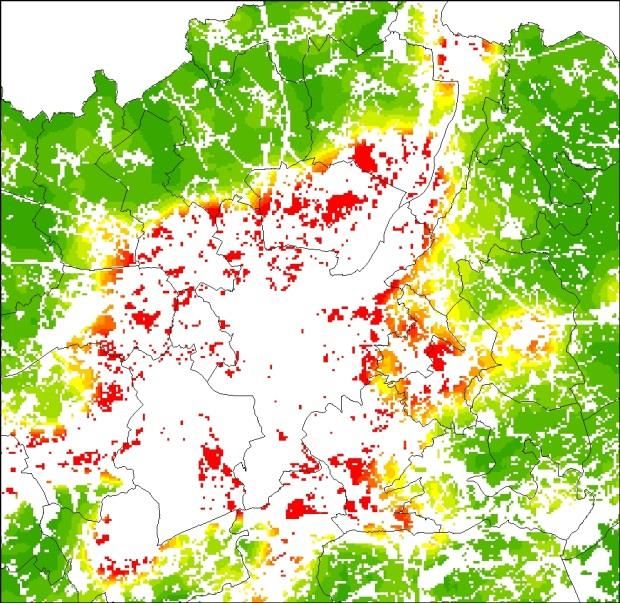
Table of Contents

 II

List of Figures

LIST OF FIGURES

Figure 1 General structure of the CCA-model: hierarchical embedded sub-models at three levels.
 The regional level is skipped in the ACA-based modelling approach _____________________ 9
Figure 2 Structure of the variable grid (Source: Crols, 2017) ______________________________ 10
Figure 3 Components of the ACA-model (Source : Crols, 2017) ____________________________ 11
Figure 4 Growth of built-up area in the Walloon region for the period 1985-2017 in ha/day (Source :
 Occupation du sol selon le Registre cadastral, Statistics Belgium, 2018) _________________ 13
Figure 5 Relative growth of residential area vs. relative population growth (1985 = 1) (Source :
 Utilisation du Sol , Statistics Belgium, 2018) _______________________________________ 14
Figure 6 Evolution of number of inhabitants per ha of residential land (Source : Utilisation du Sol,
 Statistics Belgium, 2018) ______________________________________________________ 15
Figure 7 Growth of residential area in the Walloon region for the period 1985-2017 in blue (Source :
 Utilisation du Sol, Statistics Belgium, 2018) and for the period 2018-2050 according to a BAU-
 scenario in red ______________________________________________________________ 15
Figure 8 Evolution of land use of economic sectors in the Walloon region (Source : Utilisation du
 Sol, Statistics Belgium, 2018) __________________________________________________ 16
Figure 9 Evolution of employment (left) and land use area (right) according to the BAU scenario
 (Source : PLANET model, FPB, 2015) _____________________________________________ 17
Figure 10 Growth of residential area in the Walloon region for the period 2008-2017 in according to
 a STOP-scenario (Source : Utilisation du Sol, Statistics Belgium, 2018) __________________ 18
Figure 11: Reclassified land use map ________________________________________________ 21
Figure 12 Suitability maps of the SmartPop model for residential land (upper), broadleaf forest
 (middle) and cropland (lower) _________________________________________________ 24
Figure 13 Zoning maps of the SmartPop model for residential (upper) and industry (lower) _____ 27
Figure 14 Accessibility towards the road network ______________________________________ 29
Figure 15 Growth per day of urban land in the Walloon region. In green: historic trends, in orange:
 scenario according to a business-as-Usual development, in blue: according to a ‘stop au béton’
 scenario. __________________________________________________________________ 31
Figure 16 Total land-use change 2008-2050 for the BAU and STOP scenario in the Walloon region
 __________________________________________________________________________ 31
Figure 17 Growth of the residential area in the period 2008-2050 in the BAU (upper) en STOP
 (lower) scenario. In grey: existing residential cells, in red: newly developed residential cells by
 2050______________________________________________________________________ 32
Figure 18 Residential growth in period 2008-2050 in hectares (upper) and in percentage (lower) for
 the BAU and STOP scenario ___________________________________________________ 33
Figure 19 Urbanisation rate per day for period 1985 – 2015 (based on cadastral information) and
 2015 – 2050 (based on model results of SmartPop model and RuimteModel Vlaanderen) __ 34
Figure 20: Population density in 2008 and 2050 (BAU) near Liège _________________________ 35
Figure 21 Change in population density per cell between BAU 2050 and STOP 2050 in the Walloon
 region and in the surroundings of Liège and Verviers . Values in blue represent locations with a
 higher population density in the STOP scenario compared to the BAU scenario __________ 36
Figure 22 Urban typology in the Walloon region and near Charleroi in 2008 _________________ 38
Figure 23: Zoom of the indicator map ‘Degree of urbanisation’ in 2008 and 2050 near Liège ____ 39
Figure 24 Growth of urbanisation degree towards 2050 (BAU scenario). In red: higher urbanisation
 degree in 2050 _____________________________________________________________ 40
Figure 25: Zoom of the indicator map ‘Cluster size of the built-up areas’ in 2008 and 2050 near
 Liège _____________________________________________________________________ 41
Figure 26 Cluster size distribution of urban clusters in 2008 and 2050 according to the BAU and
 STOP scenario ______________________________________________________________ 41

 III

List of Figures

Figure 27: Zoom of the indicator map ‘Cluster size of open space‘ in 2008 and 2050 near Liège__ 42
Figure 28 Cluster size distribution of clusters of open space in 2008 and 2050 according to the BAU
 and STOP scenario __________________________________________________________ 43
Figure 29: Zoom of the indicator map ‘Distance to railway stations’ in 2008 and 2050 near Liège.
 Railway stations are the black dots in the map. ____________________________________ 44
Figure 30: Zoom of the indicator map ‘Urban pressure on agricultural land’ in 2010 and 2050 near
 Liège _____________________________________________________________________ 46
Figure 31 UrbClim land use map for the Liège model domain. ____________________________ 48
Figure 32 The mean 2m air temperature in Liège during the summer months for the years 1996-
 2015. _____________________________________________________________________ 49
Figure 33 The mean Urban Heat Island in Liège at 23h during the summer months for the years
 1996-2015. ________________________________________________________________ 50
Figure 34 The mean Urban Heat Island in Liège at 23h during the summer months for the years
 1996-2015, corrected for topographic effects. ____________________________________ 51
Figure 35 The expected temperature increases for the 21st century from different emission
 scenarios according to the global climate models of the IPCC. ________________________ 52
Figure 36 The mean 2m air temperatures in Liège during the summer months for the years 2026-
 2045 (left) and 2081-2100 (right) according to the RCP8.5 scenario. ___________________ 52
Figure 37 Evolution of the number of heat wave days per year according to the RCP8.5 scenario. 53
Figure 38 Population exposure to heat waves for 2010 and 2030 according to the BAU-scenario 54
Figure 39 : Double fonction conditionnelle, schéma conceptuel ___________________________ 59
Figure 40 : Classes de pentes ______________________________________________________ 60
Figure 41 : Exposition ____________________________________________________________ 61
Figure 42 : Risque d’érosion des sols ________________________________________________ 62
Figure 43 : Aléa d’inondation ______________________________________________________ 63
Figure 44 : Protection des zones de captages _________________________________________ 64
Figure 45 : (a, b, c) : Secteurs forestiers optimaux ______________________________________ 70
Figure 46 : Aptitudes aux cultures __________________________________________________ 72
Figure 47 : Aptitude - Friches industrielles ____________________________________________ 75
Figure 48 : Aptitude - Friches agricoles ______________________________________________ 75
Figure 49 : Aptitude - Zones de cultures _____________________________________________ 76
Figure 50 : Aptitude - Vergers & vignobles____________________________________________ 76
Figure 51 : Aptitude - Prairies ______________________________________________________ 77
Figure 52 : Aptitude - Terrils & terrains vagues ________________________________________ 77
Figure 53 : Aptitude - Zones récréatives _____________________________________________ 78
Figure 54 : Aptitude - Résidentiel ___________________________________________________ 78
Figure 55 : Aptitude - Industrie ____________________________________________________ 79
Figure 56 : Aptitude - Services _____________________________________________________ 79
Figure 57 : Aptitude - Commerces __________________________________________________ 80
Figure 58 : Aptitude - Exploitations agricoles __________________________________________ 80
Figure 59 : Aptitude - Forêts de feuillus _____________________________________________ 81
Figure 60 : Aptitude - Forêts de conifères ____________________________________________ 81
Figure 61 : Aptitude - Forets mélangées _____________________________________________ 82
Figure 62 : Contraintes karstiques __________________________________________________ 83
Figure 63 : Zonage - Friches industrielles _____________________________________________ 87
Figure 64 : Zonage – Friches agricoles _______________________________________________ 87
Figure 65 : Zonage - Zones de culture _______________________________________________ 88
Figure 66 : Zonage - Vergers & vignobles _____________________________________________ 88
Figure 67 : Zonage – Prairies ______________________________________________________ 89
Figure 68 : Zonage - Terrils & terrains vagues _________________________________________ 89
Figure 69 : Zonage - Zones récréatives _______________________________________________ 90

 IV

List of Figures

Figure 70 : Zonage – Résidentiel ____________________________________________________ 90
Figure 71 : Zonage – Industrie______________________________________________________ 91
Figure 72 : Zonage – Services ______________________________________________________ 91
Figure 73 : Zonage – Commerces ___________________________________________________ 92
Figure 74 : Zonage - Exploitations agricoles ___________________________________________ 92
Figure 75 : Zonage - Forêts de feuillus _______________________________________________ 93
Figure 76 : Zonage - Forêts de conifères ______________________________________________ 93
Figure 77 : Zonage - Forets mélangées _______________________________________________ 94

 V

List of Tables

LIST OF TABLES

Table 1: The land uses at the Local level of the model __________________________________ 19
Table 2 Input maps used to create the suitability maps for the different land-use types ________ 22
Table 3 Input maps used to create the zoning maps for the different land-use types. X indicates
 whether the specific criterion is taken into account for the specific land-use type. ________ 25
Table 4 Translation of ‘plans de secteur ‘to zoning status in the SmartPop model _____________ 26
Table 5 Urban typology (based on Charlier & Reginster, 2018) ____________________________ 37
Table 6 Effect of both scenarios on the number of inhabitants per urban type _______________ 38
Table 7 Average distance of residential cells towards closest railway station per arrondissement 45
Table 8 Translation of the SmartPop land use classes to the UrbClim classes and their respective
 parameter values. ___________________________________________________________ 46

 VI

CHAPTER 1 BACKGROUND AND OBJECTIVES

The prime objective of the work carried out in WP4 is the development and application of a
Constrained Cellular Automata-based (CCA) land use model for the Walloon region.

In the last 10 years, VITO has already implemented and applied several CA-models within Belgium:
  In Flanders, the RuimteModel Vlaanderen dates back to 2007 and is currently still under
 development and upgraded by VITO. This CCA-based land use model is used for decision
 support by several Flemish government administrations and agencies, including the Spatial
 Development Department, the Agency for Nature and Forests, the Flemish Environment
 Agency etc. Several versions of the RuimteModel exist in which Flanders and the Brussels-
 Capital Region are modelled at a spatial resolution up to 1 hectare and taking into account up
 to 81 different land-use types.
  Within the Belspo-SSD MULTIMODE project, a CCA-based land-use model ahas been built for
 the whole of Belgium. Compared to the RuimteModel Vlaanderen, however, this model is
 limited in its spatial (300x300m) and thematic (20 land-use types) resolution.
  Within the Belspo-SSD GroWaDRISK project an Activity-based CA-land use model (ACA) for
 the whole of Belgium is under construction. ACA-types of land-use model differ from CCA-
 based land use models in the way they deal with spatial interaction at the regional level.

One of the goals of the SmartPop project is to develop a CA-based land-use model for the Walloon
region, similar to the RuimteModel Vlaanderen. Hereto, the maximum use is made of the Flemish’
knowledge and experience to use this type of models for policy-support. Therefore, a similar
approach will be applied in both regions since this is interesting for integrated planning.
Homogenizing risks studies between regions is intended since natural hazards are not stopped by
regional borders.

At the start of the SmartPop project, the RuimteModel was a Constrained Cellular Automata (CCA)
type of land-use model (White et al., 2015). The first prototype of the SmartPop model was
implemented and calibrated within this framework

However, during the course of the project, the RuimteModel Vlaanderen was re-implemented as an
activity-based cellular automata (ACA) based land-use model (White et al. 2012; Crols et al, 2017).
With a view to use similar methodologies in both Wallonia and Flanders, the choice was made to re-
implement the first SmartPop prototype to an ACA-model as well. Another advantage of using an
ACA-approach is that yearly population dynamics, which is an essential part of the SmartPop project,
are an intrinsic element in the model. Ssince the model intrinsically deals with population (as an
activity), the model is very suitable to be used to explore the effect of various proposed policies on
the spatial distribution of population, and in particular on the annual total land take for new housing.
Hereto, the population map of WP 3 is used as an input map in the model.

This report gives an overview of the general modelling concept used in the ACA-based land-use
model (CHAPTER 2), of the main inputs and parameters used in the Walloon application (CHAPTER 3)
and its main results (CHAPTER 4 and CHAPTER 5).

 18/08/2017 – v9 7

CHAPTER 2 GENERAL MODELLING CONCEPT

In this chapter a general methodological outline of the ACA-based land-use model is presented.
CHAPTER 3 will dwell more extensively in specific Walloon application and will describe the main
inputs and parameter settings of the model.

The kernel of the SmartPop model is an activity-based cellular automata based land-use model (ACA
model) operating at a spatial resolution of 1ha. The SmartPop ACA-model is an implementation of
the ACA-model originally developed by White, Uljee and Engelen (2012) and further improved by
Crols (2017). Cellular automata (CA) have perhaps been the most popular way to model land-use
change and spatially-explicit population density because (i) they are intrinsically dynamic, (ii) they are
able to deal with high resolutions and thus produce results with a useful amount of detail and (iii)
they outperform other models in realistically modelling land-use change. Recently, White, Uljee and
Engelen (2012) proposed an activity-based model of urban dynamics, which directly models spatial
changes in the density of different activities (such as population and employment in several
economic sectors) instead of land-use categories.

The approach is activity based rather than land-use based. Although land use plays a role in the cell
transition process and is also one of the outputs of the model, model processes are defined
essentially in terms of activities. Moreover, a single cell can have multiple. This activity-based
approach is therefore an interesting alternative to handle mixed and multifunctional land use.
In principle, land use corresponds to the dominant activity on a cell (e.g. residential land use
corresponds with population). However, while many land uses (e.g. pasture, forest) may not have an
activity level associated with them in a particular model application, they can nevertheless have
secondary activities (i.e. those not corresponding to the current land use) assigned to them. For
example, cells with forest or pasture can have (small numbers of) activities such as population and
commercial employment, assigned.

The scenario that drives a simulation provides for each activity K a proportion QK that is located as
primary activity, i.e. located on cells of the land use that corresponds to the activity. The remaining
proportion of the activity, 1-QK, is located as secondary activity, i.e. located on cells that do not have
the associated land use (e.g. population as a secondary activity on cells with a commercial land use).
Also provided as input parameters are compatibility factors that express the relative compatibility of
each activity with each land use type.

Land uses are divided into three categories: active, passive, and fixed. Active land uses are those
that have associated activities—e.g. residential land use is associated with population. These are the
categories for which activity potentials are calculated for all cells on the map. Activities are
distributed and land uses are changed in function of these potentials. Passive land uses are those
without associated activities and which therefore do not have their own change dynamic; cells with
these states change only when they are converted to one of the active land use states. Finally, fixed
states are those which do not change at all as a result of the model dynamics. While passive and
fixed land use states do not have their own active dynamics, they can influence the transition
potentials of the active states by being included in the matrix of influence weights used to calculate
the neighbourhood effect.

 18/08/2017 – v9 8

While the CCA-based land-use model, which was used in the first prototype of the SmartPop model,
was operating at three hierarchically embedded geographical levels (see Figure 3), the ACA-based
land-use model is only operating at two levels: (1) a global level in which regional trends (i.e. at the
level of the entire Walloon region) of activity and land-use change are used as inputs and (2) a
cellular level (1ha resolution) at which the land use and activities are being modelled. In the ACA-
model, the regional level is thus skipped and global demands are directly translated to local (1ha
resolution) changes in land use and activity using a Cellular Automat. In this Cellular Automat land-
use change is triggered by means of transition potentials. These potentials for future land-use are
mainly determined by the neighbourhood effect of the ACA model, a function representing the
influence of activities and land uses on each other at different distances. This neighbourhood effect
includes influences at all scales and distances within the study area. To make this computationally
feasible, cell values are grouped into super-cell values in a variable grid structure (Figure 2): the
further away from the focus cell for which the neighbourhood effect is being computed, the larger
the super-cell (White, 2006). The influence rules in the variable grid are depending on travel time
between the (super)cells instead of Euclidian distance, which are usually used in CA-types of model.

 Figure 1 General structure of the CCA-model: hierarchical embedded sub-models at three levels. The
 regional level is skipped in the ACA-based modelling approach

 18/08/2017 – v9 9

Figure 2 Structure of the variable grid (Source: Crols, 2017)

In the ACA-based model transition potentials VKi on a cell i are computed for each activity K for each
annual time step:
 VKi = r ZKi SKi XKi NKi (Equation 1)
With:
  r a random perturbation term,
  ZKi the zoning status,
  XKi the accessibility to the transport network,
  SKi the physical suitability, and
  NKi the neighbourhood effect.

The neighbourhood rules are a function of travel time between the focal cell and a variable grid cell
that influences the focal cell:

 NKi = ∑J ∑j WJK,dij (TJj / TJ)(Equation 2)

With:
  WJK,dij the weight given by the influence function fJK for the influence of activity J on activity K
 at (time) distance dij,
  TJj the total activity J on variable grid cell j, and
  TJ the total activity J in the study area.

Travel times are computed between the centres of gravity of population of the variable grid cells.

The land-use transition potential VTKi for the associated active land use UK on cell i is calculated as:
 VTKi = DKi (VKi)mK + (IK)ρ (Equation 3)
With:
  DKi the diseconomies of agglomeration, representing the effect of high land prices and
 congestion on locational decisions,

 18/08/2017 – v9 10

 mK parameters to be calibrated,
  IK is the inertia value, which deals with the tendency of land uses to remain fixed at a
 location, and
  ρ is a parameter to decrease inertia outside the associated land use of activities.

Next, all cells are ranked by their highest potential for a land use. The transition rule gives each cell
the land use for which it has the highest potential until there is no more demand for that land use.

Activity values TKi are updated to T’Ki in two steps, followed by a rescaling operation to ensure that
total demand values are respected. Firstly, the allocation of activity in cells with a changed land-use
state is in proportion to the relative value of the activity potential VKi within all cells of this land-use
state. Next, activity is increased in cells with a high neighbourhood effect, by calibrating a
densification exponent.
More information on the ACA-model can be found in Crols (2017).

Figure 3 shows a schematic overview of the workflow of the model and of the different components
of the ACA-model.

 Figure 3 Components of the ACA-model (Source : Crols, 2017)

 18/08/2017 – v9 11

CHAPTER 3 APPLICATION OF THE ACA LAND-USE MODEL IN THE WALLOON
 REGION

The base year of the SmartPop model application is 2008. This is the year for which the land-use map
is available (COSW, see further) as well as the statistical data that are used to drive the model at the
global level. The simulation iterates in yearly time steps. For every year, up to 2050, output can be
generated and stored.

As is shown in Figure 3, the ACA-model is driven by a demand for activity on the one hand and a
demand for land on the other hand. These demands represent trends at the level of the entire
Walloon region and are thus treated as the ‘global level’ of the ACA-based model. At the ‘local’,
cellular level of the ACA-based model, these global demands are translated to cells at a 1ha scale
level.

In this chapter, the different inputs at both levels are described.

3.1. GLOBAL LEVEL: DEMAND FOR ACTIVITY AND DEMAND FOR LAND

In the SmartPop application, 4 types of activities are being modelled: population, employment in
industry, employment in services and employment in commerce. These activities are associated as
primary activity with 4 ‘active’ land-use types: residential, industry, services and commerce.

The model is fed with two types of inputs for each of these 4 land-use types for the time period
which is being modelled:
(1) area demands (yearly growth in hectares) for residential and economic land-use types and
(2) yearly population and employment numbers.

The other 4 ‘active’ land-use types in the SmartPop model (farm houses, deciduous forest, coniferous
forest and mixed forest) are not associated with a primary activity and are solely driven by area
demands.

In the SmartPop project two scenarios are simulated using the ACA-model: a Business-as-Usual
scenario (BAU) and a ‘Stop au béton’ scenario (STOP). These scenarios differ in the set inputs trends
at the global level. Both scenarios use the same trends for population and employment growth, so
the same demands for activity, which are based on the prognoses of the Federal Planning Bureau.
The scenarios, however, show different area demands for residential and economic development. In
the context of a ‘stop au béton’, no more urban expansion will take place by 2050. This means that
new inhabitants should find a place to live without creating new residential areas and thus that a
thorough densification of the existing residential area will be needed by 2050.

 18/08/2017 – v9 12

3.1.2. AREA DEMANDS IN BUSINESS-AS-USUAL SCENARIO

 Decreasing population densities

Since the 1980s, the Walloon region has ‘artificialized’ at a rate of 4.6 ha/day (Charlier & Reginster,
2017; Statistics Belgium, 2018). Although this average growth rate has decreased from more or less
5.5 ha/day in the 1990s, over 4.3 ha/day in the period 2000-2010, to 3.3 ha/day in the last decade
(Figure 4), the rate of urban growth is still relatively high, compared to the growth rate of the
population in the same period. While there was a 60% growth of residential land in the period 1985 -
2015, the population increased with more or less 10% in the same period (Figure 5).

 Figure 4 Growth of built-up area in the Walloon region for the period 1985-2017 in ha/day (Source :
 Occupation du sol selon le Registre cadastral, Statistics Belgium, 2018)

 18/08/2017 – v9 13

Figure 5 Relative growth of residential area vs. relative population growth (1985 = 1) (Source :
 Utilisation du Sol , Statistics Belgium, 2018)

As a result, the number of inhabitants per hectare of residential land is decreasing in time, or the
land uptake per person has increased. While the average population density in the Walloon region
was still 55 inhabitants per hectare of residential land in 1985, this has decreased to 36.5 inhabitants
per hectare of residential land in 2017 (Figure 6).

However, the observations also show that this trend of further decreasing population densities is
slowly coming to a stop (Figure 4). Or in other words, nowadays the growth of the built-up land is still
outperforming the growth of the population, but to a lesser degree than in the 1980s and 1990s.

In the Business-as-Usual (BAU) scenario we assume that the further decrease of the population
densities will come to a stop and that the population densities will remain more or less constant at
the current density of 35 inhabitants per hectare of residential land.

This average population density, combined with the population growth projections of the Federal
Planning Bureau (FPB, 2017) of 375.000 inhabitants by 2050, give a further growth of residential land
in the Walloon region by 2050 of more or less 16.000 hectares, with an average growth rate in the
period 2018-2050 of 1,3 ha/day (Figure 7).

 18/08/2017 – v9 14

Figure 6 Evolution of number of inhabitants per ha of residential land (Source : Utilisation du Sol,
 Statistics Belgium, 2018)

Figure 7 Growth of residential area in the Walloon region for the period 1985-2017 in blue (Source :
 Utilisation du Sol, Statistics Belgium, 2018) and for the period 2018-2050 according to a BAU-
 scenario in red

 18/08/2017 – v9 15

 Growth of the industry, commerce and services

Besides the growth of the residential land, urban expansion is also driven by growth of the area
needed for industry, services and commerce. These built-up categories have also known a substantial
growth in the past (Figure 7).

For each type of economic land use the current job densities (number of employees in an economic
sector over the area occupied by the sector) are calculated. These job densities are: +/- 10 employees
/ ha for industry, +/- 75 empoyees / ha for services and +/- 63 employees / ha for commerce. Both
for the sectors industry and commerce these densities have proven to be quite stable during the last
decades. The sector of the public services, however, has known an increase of the average job
density over the last 5 years of about 71 employees / ha in 2013 to 75 employees / ha in 2018. The
BAU scenario builds upon these observations. Towards 2050 the scenario assumes constant job
densities in the sectors industry and commerce and a further increase of the job density up to 80
employees per hectare in 2025 for the public services. This density of 80 employees per hectare is
kept constant up to 2050.

These densities are combined with projections of employment development per economic sector
from the PLANET model of the Federal Planning Bureau (FPB, 2015, Figure 9, left). This results in an
increased area for services in 2050 (mainly due to the rather large growth of the employment in the
sector by 2050), a small decrease for the area of commerces (due to the increased job density by
2050 and the rather small growth in employment in the sector) and a status quo for the area of
industry (decrease in employment by 2050 combined with decreasing job density). Figure 9 (right)
shows the evolution in the land-use area of the economic sectors. These area demands are used as
input at the global level of the model.

 Figure 8 Evolution of land use of economic sectors in the Walloon region (Source : Utilisation du Sol,
 Statistics Belgium, 2018)

 18/08/2017 – v9 16

Figure 9 Evolution of employment (left) and land use area (right) according to the BAU scenario
 (Source : PLANET model, FPB, 2015)

3.1.3. AREA DEMANDS IN THE STOP AU BÉTON SCENARIO

In the ‘stop au béton’ (STOP) scenario the same trends for population and employment growth are
used as in the BAU scenario. The scenario differs from BAU in the area of new urban land which will
be developed by 2050. In the STOP scenario, the current growth of 4.6 ha/day decreases to 1.64
ha/day in 2025 (or 6km² per year) and further to 0 ha/day in 2050 (Figure 10). This leads to more or
less 14.000 ha of new urban development by 2050. This is around 4.000 ha less than in the BAU
scenario. This total growth is divided over the residential sector and the economic sectors, which will
all evolve towards a zero growth in 2050. As a consequence, the average population densities in the
residential area will have to increase substantially compared to a BAU-scenario.

 18/08/2017 – v9 17

Figure 10 Growth of residential area in the Walloon region for the period 2008-2017 in according to a
 STOP-scenario (Source : Utilisation du Sol, Statistics Belgium, 2018)

3.1.4. AREA DEMANDS FOR LAND-USE TYPES, NOT ASSOCIATED WITH ACTIVITIES

While economic and population figures are posed in terms of numbers of people, or jobs, the natural
land-use categories are expressed in terms of total area occupied. The area occupied by natural land-
use categories is imposed by means of scenarios. This is justified by the fact that the expansion of
areas occupied by natural land-use is in general an act of deliberate policy, rather than a
spontaneous process. There are three natural land use classes in the SmartPop model, (1) deciduous
forests, (2) coniferous forests, and (3) mixed forests. Since good insights about possible future forest
transitions were lacking, the areas for the three types of forests are assumed to be constant in time
in both scenarios. This means that if existing forest land is changed to urban land, this area has to be
compensated for at another location.

3.2. LOCAL LEVEL

At the Local level, the Walloon region is represented as a raster of 1.689.798 cells. The cells measure
100 by 100 meter (1 ha). The land use map used by the Local model is based on the Carte d’
Occupation du sol de Wallonie.

As was described in CHAPTER 2 transition potentials VKi determine whether a cell is taken in by a
particular activity. This transition potential is a function of four elements (Figure 3):
 The neighbourhood effect represents the impact of land uses and activities in the area
 immediately surrounding a location. The presence of complementary or competing activities and
 desirable or repellent land uses is of great significance for the quality of a location and thus for its
 appeal to particular activities. For each cell, the model assesses the quality of its neighbourhood
 within the variable grid.
 Physical suitability is represented in the model by one map per ‘active’ land-use category. The
 term suitability is used here to describe the degree to which a cell is fit to support a particular
 land-use function and the associated economic or residential activity. The maps are prepared
 within a GIS.
 Zoning or institutional suitability is also characterized by one map per ‘active’ land-use category.
 It is another composite measure based on master plans and planning documents available from
 national or regional planning authorities including: ecologically valuable and protected areas,
 protected culturescapes and buffer zones. For maximally three consecutive planning periods,
 determined by the user (e.g.: 2008-2015, 2015-2020 and 2020-2050), each zoning map specifies
 which cells can and cannot be taken in by the particular land use. The maps are prepared within a
 GIS.
 Accessibility relative to the transportation infrastructure for each land-use function is calculated.
 It is an expression of the ease with which an activity can fulfil its needs for transportation and
 mobility in a particular cell. It accounts for the distance of the cell to the nearest link or node on
 each of the networks, the importance and quality of that link or node, and the particular needs
 for transportation of the activity or land-use function.

These different input maps and input data and the specific implementation for the Walloon context
are further described below. The other model parameters (neighbourhood rules, diseconomies,
inertia) are calibrated based on expert-judgement.

 18/08/2017 – v9 18

The most important input of any land-use model is off course a land-use map. Besides a land-use
map, the ACA-model also needs activity maps for population and employment in different economic
sectors.

3.2.1. LAND USES

The land-use map is derived from the Carte d’ Occupation du sol de Wallonie (COSW, 2007). This is a
vector-maps which distinguishes 71 land cover classes at its most detailed level (level 5). Not all
classes are however relevant to the model. Moreover, the more land-use categories that need to be
taken into account, the more effort is needed for calibrating the model. Therefore, a simplification of
the original COSW legend with 71 categories to land-use map with 26 categories was performed.
Therefore a number of preprocessing steps had to be conducted on the original COSW:
 1. Vector to raster (10x10m) translation: in a first step the 71 land use classes were rasterised
 to a grid with cell sizes of 10 by 10 meters.
 2. Aggregation of the original 71 land use types to 26 land use categorie which are used at the
 local level (see Table 1). This original COSW categories ‘Autres terrains artificialisés’ (category
 15), ‘Bandes enherbées’ (category 233) and ‘Non classé’ (category 9) are attributed to the
 largest neighbouring land use class.
 3. Resampling of the 10x10m land use raster map to a 100x100m resolution under the
 constraint of a conservation of area for each land use categorie. This was done using the
 SpatAggr tool developed by RIKS NV.

Table 1 lists the 26 land uses which have currently been retained in the model as well as the areas
they occupy at a 1ha resolution. The choice of the 26 categories is based on the RuimteModel
Vlaanderen, which takes a similar set of land-use categories into account.

From the 26 land-use types, eight are treated as ‘active’ land-use types (residential land, industry,
commerces, services, farm houses, decidious forests, coniferous forests and mixed forests). These
categories are thus dynamically modelled in time. Seven land use categories are treated as ‘passive’
land-use types: brownfields, barren land, cropland, orchards, pastures, other open land and
recreation. The areas of these land use types can thus change in time, but the changes are mainly
driven by the active types. Cropland, for instance, can disappear in favor of residential growth.
Finally, 11 land use categories are treated as fixed: these land use types remain static in time. They
include: heathland, grasslands, wetlands, parks, aeroports, extraction sites, landfills, military services,
ports, infrastructure and water.

 Table 1: The land uses at the Local level of the model

Land use categorie COSW categories Type Area
Brownfields 1341 – 1342 Passive 3167.89
Barren land 25 Passive 8188
Croplands 21110 – 21111 – Passive 415788.97
 21112 – 21113 –
 2112 – 21131 –
 21132
Orchards 2221 - 2222 Passive 8985.95
Pastures 2311 – 2312 – Passive 461420.55
 232
Other open land 3242 – 325 Passive 28586.71
Recreation 1242 – 14211 – Passive 6932.13

 18/08/2017 – v9 19

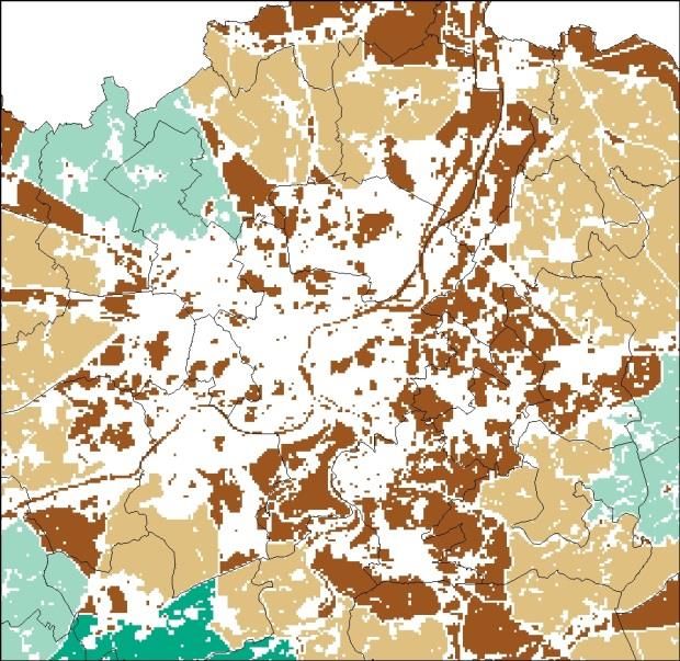
14212 - 1422
Residential 1111 – 1112 – Active 98621.49
 11211 – 11212 –
 11213 – 11214 –
 11215 – 11216 –
 11221 – 11222 –
 11223
Industry 12111 - 12112 Active 15724.32
Services 12121 – 12122 – Active 10078.64
 12123 -12124 –
 12127 – 12128 –
 12129 - 12134
Commerce 12131 – 12132 – Active 3659.01
 12133
Farm houses 12141 - 12142 Active 9037.96
Decidious forest 311 Active 168438.66
Coniferous forest 312 Active 120200.12
Mixed forest 310 – 313 Active 192506.85
Heathland 322 Fixed 496.7
Grasslands 321 Fixed 5770.02
Wetlands 411 - 412 Fixed 5426.14
Parks 12125 - 141 Fixed 5548.38
Aeroports 1241 Fixed 333.35
Extraction sites 1311 - 1312 Fixed 10878.67
Landfills 132 Fixed 323.84
Military Services 12126 Fixed 6159.88
Port 123 Fixed 525.43
Infrastructure 1221 - 1222 Fixed 79293.48
Water 5111 – 5112 - 512 Fixed 16654.44

The resulting land use map at the Local level is shown in Figure 11.

 18/08/2017 – v9 20

Figure 11: Reclassified land use map

3.3. ACTIVITY MAPS

In WP3 of the Smartpop project, a population map for the Walloon region was created from open
data based on dasymetric mapping. The SmartPop model uses the dasymetric map at 1 hectare
resolution as an input activity (population) map. The inputs and creation of this 1ha population map
are described in the technical report of WP3.

Besides a population map, the ACA-model also needs employment density maps for all of the three
economic sectors (industry, commerces, services) at a resolution of 1 hectare. These maps are
produced by means of a dasymetric mapping technique, similar as the one used in WP3. Hereto,
employment figures for 2008 are used at the level of the Comité Subrégional de l'Emploi et de la
Formation (CSEF).

3.4. SUITABILITY

Suitability is a spatially distributed statistic and dimensionless value on a map that expresses the
appropriateness of each cell to receive a land use in values in the interval {0, 1}. It is a composite
measure based on ecological, physical, technical or economical factors determining its physical
appropriateness. It describes, in other words, the degree to which a cell is suitable to receive a
particular land-use type. The suitability maps remain constant over time unless they are changed
interactively.

The suitability map is a map at a 1ha resolution which expresses the weighted sum of the influence of
different factors which are characterized by spatial data. The weights reflect the relative importance
of each of the factors. These weights are synthesized into a single measure which is linearly rescaled

 18/08/2017 – v9 21

to the interval {0, 10}. Table 2 gives an overview of all locational factors which have been taken into
account in the suitability maps of the different land-use types. Figure 12 gives the result for 3 land-
use types: residential land, cropland and deciduous forest. A full description of the creation of the
suitability maps and all of the resulting maps can be found in annex 1 (in French).

 Table 2 Input maps used to create the suitability maps for the different land-use types

 Coniferous forest
 Other open land

 Decidious forest

 Mixed forest
 Farm houses
 Brownfields

 Barren land

 Residential
 Recreation

 Commerce
 Croplands

 Orchards

 Pastures

 Industry

 Services
 Slope
 X X X X X X X X X X X X X X
 based on MNT LiDAR
 (2013-2014)
 Aspect (Slope
 orientation)
 X X X X X X X
 based on MNT LiDAR
 (2013-2014)

 Erosion risk
 X X X X X X X
 based on ERRUISOL
 data (SPW)

 Flood risk
 derived from flooding X X X X X X X X X X X X
 alea by overflow and
 runoff (SPW)
 Groundwater
 protection zones
 X X X X X X X X X X X X X X X
 Protection of the well
 area (SPW)

 Soils
 Map of the Main Soil X X X X X X X X X X X X X X
 Types of Wallonia
 (CNSW20)

 Lans Use
 X X X X X X X X X X X X X X X
 land-use map of the
 SmartPop model
 Optimal forest
 locations
Based on "Definition of X X X
 the aptitude of forest
 stations" (1991).

 18/08/2017 – v9 22

Suitability for arable
 land
 X X X
 (PCNSW, 2007)

 18/08/2017 – v9 23

Figure 12 Suitability maps of the SmartPop model for residential land (upper), broadleaf forest
 (middle) and cropland (lower)

3.5. ZONING

Zoning (ZMl,c) is a spatially distributed statistic dimensionless value on a map that shows in a binary
manner whether a cell can (= 1) or cannot (= 0) be occupied by a certain land use. Zoning maps
represent the legal possibility to develop a certain land-use type at a certain location. The zoning
maps show whether a specific location at a 1 ha resolution can or cannot be occupied by a certain
land use at a certain point in time. The zoning can thus change in time and space. The model allows
making a distinction between three planning periods per land use:
  Zoning period zp = 0: from start date (t=t0) till first data set (t=t1).
  Zoning period zp = 1: from first date set (t=t1) till second date set (t=t2).
  Zoning period zp = 2: from second date set (t=t2) till end date of simulation t=T)
In the SmartPop model, a distinction between three planning periods is made:
  zp = 0: 2008-2015,
  zp = 1: 2015-2025 and
  zp = 2: 2025-2050.

In numbers varying from 0 to 3, the zoning maps, ZMl,c, indicate for each cell from which period
onwards the land use is allowed in the cell:
  ZMl,c = 0: the land use is allowed starting in 2008 until the end of the simulation (2050), so
 throughout the entire modelled period
  ZMl,c = 1: the land use is allowed starting in 2015 until the end of the simulation (2050),
  ZMl,c = 2: the land use is allowed starting in 2025 until the end of the simulation (2050), and
  ZMl,c = 3: the land use is never allowed

By using these different time frames, expected changes in the planning status of documents can be
adopted in the model. These include, for instance, expected changes in the protection status of
natural reserves (can be more strict or less strict in the near future), or expected changes in the
effect of spatial plans.

 18/08/2017 – v9 24

It is assumed, moreover, that the change in the zoning status of a cell from not allowed (0) in the
present zoning period to allowed (1) in the next zoning period, or vice versa, is gradual. Hence, that a
change in the zoning status is anticipated and a cell will change state as a function of the elapsed
time in the present zoning period. The gradual change in the zoning status has the technical
advantage over a sudden change in that it avoids an unrealistic behaviour of the model during the
first time step of a new planning period (when suddenly a lot of newly zoned land may become
available: this can cause a ‘leap’ in the land use changes, which is unrealistic). It thus represents
reality much better in that the zoning status of land is changing gradually within broadly defined
planning periods.

The parameter ζ expresses this level of anticipation of the future zoning status. High values (1

1 Brownfields x x x x x x x x x x
 2 Barren land x x x x x x x x
 3 Croplands x x x x x x x x
 4 Orchards x x x x x x x x
 5 Pastures x x x x x x x x
 6 Other open land x x x x x x x x x
 7 Recreation x x x x x x x x x x
 8 Residential x x x x x x x x x x
 9 Industry x x x x x x x x x x
 10 Services x x x x x x x x x x
 11 Commerces x x x x x x x x x x
 12 Farm houses x x x x x x x x x
 13 Decidious forest X X
 14 Coniferous forest X X
 15 Mixed forest x x

 Table 4 Translation of ‘plans de secteur ‘to zoning status in the SmartPop model

 Coniferous forest
 Other open land

 Decidious forest

 Mixed forest
 Farm houses
 Brownfields
 Barren land

 Residential
 Recreation

 Commerce
 Croplands
 Orchards
 Pastures

 Industry
 Services

A01 Activité économique mixte 0 3 3 3 3 3 1 1 0 0 0 3 0 0 0
A02 Activité économique industrielle 0 3 3 3 3 3 1 1 0 0 0 3 0 0 0
A11 Activité éco. spécifique agro-économique 0 0 0 0 0 3 1 1 0 0 0 0 0 0 0
A12 Activité eco. spécifique grande distribution 0 3 3 3 3 3 1 1 1 1 0 1 0 0 0
D01 Aménagement communal concerté 3 3 1 1 1 3 1 1 1 1 1 1 0 0 0
D02 Aménagement communal concerté à caractère industriel 1 3 3 3 3 3 3 3 1 1 1 3 0 0 0
E01 Plan d'eau 3 3 3 3 3 3 3 3 3 3 3 3 3 3 3
H01 Habitat 3 3 0 0 0 3 0 0 3 3 0 0 0 0 0
H02 Habitat à caractère rural 3 3 0 0 0 3 0 0 3 3 0 0 0 0 0
L01 Loisirs 3 3 3 3 3 3 0 3 3 0 0 3 0 0 0
P01 Services publics et équipements communautaires 3 3 3 3 3 3 3 1 1 0 1 0 0 0 0
P02 Centre d'enfouissement technique 3 3 3 3 3 0 3 3 3 3 3 3 2 2 2
P11 Servitude particulière 3 3 3 3 3 3 3 3 3 3 3 3 0 0 0
P12 Non affecté ("zone blanche") 0 0 0 0 0 0 0 0 0 0 0 0 0 0 0
R01 Agricole 3 0 0 0 0 0 3 3 3 3 3 0 0 0 0
R02 Forestière 3 0 3 3 3 3 3 3 3 3 3 3 0 0 0
R03 Espaces verts 3 3 3 3 3 3 3 3 3 3 3 3 0 0 0
R04 Naturelle 3 3 3 3 3 3 0 3 3 3 3 3 0 0 0
R05 Parc 3 3 3 3 3 3 3 3 3 3 0 3 3 3 3
V01 Vierge de toute affectation (annulation du Conseil Etat) 0 0 0 0 0 0 0 0 0 0 0 0 0 0 0

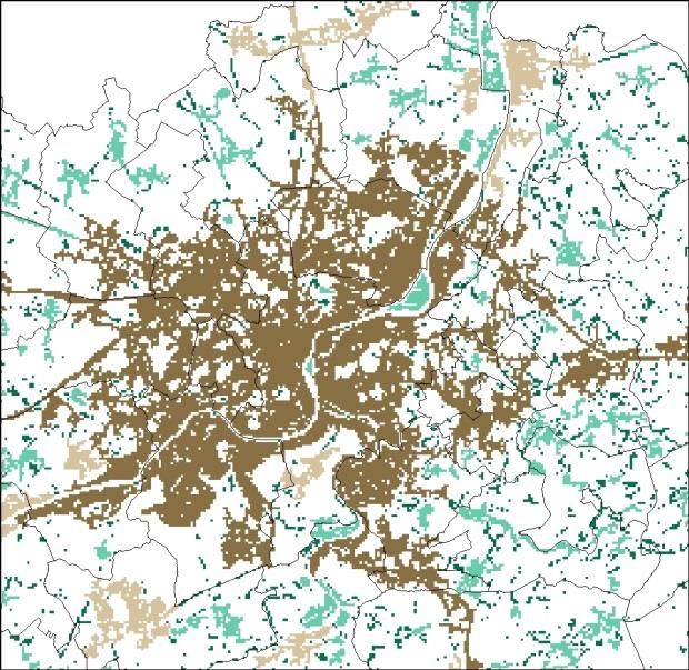
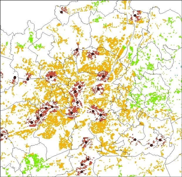
 18/08/2017 – v9 26

X01 Extraction 0 3 3 3 3 3 1 3 2 3 3 3 2 2 2

 Figure 13 Zoning maps of the SmartPop model for residential (upper) and industry (lower)

3.6. ACCESSIBILITY

Accessibility is a spatially distributed measure (on a map) expressing, in values ranging between 0
and 1, the degree to which a cell can be accessed via the transportation infrastructure.

The local accessibility reflects the distance of a cell to the transport infrastructure. The transport
infrastructure consists of a number of networks, which may consist of either points (such as railway

 18/08/2017 – v9 27

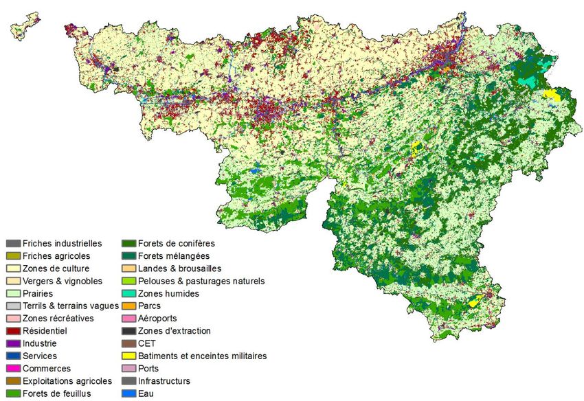
stations or access points to motorways) or lines (such as roads or canals). A cell that is positioned
closer to a line or point of a network has a higher local accessibility.

For each network the effect of proximity on accessibility is calculated according to
 1 as ,l
t
 As ,l ,c  
 D as ,l  Ds ,c
 1  s ,c
 as ,l
 (Equation 7 7).
 1 as ,l
 t
 As ,l ,c  
 D as ,l  Ds ,c
 1  s ,c
 as ,l
 (Equation 7)
with:
t
 As,l,c Accessibility of cell c for land use l concerning the network s.
Ds,c The distance of cell c to the nearest cell on the network s.
as,l The accessibility coefficient representing the importance of a good access to the network s
 for land use l. (with as,l ≥ 0). This parameter expresses for instance the fact that the
 accessibility to the infrastructure network is more important for industrial land than for
 farm houses. The decrease of the accessibility tAs,l,c will therefore be larger with growing
 distances from the infrastructure network for industrial land than for farm houses.

A special case are land use classes that suffer rather than benefit from accessibility, in particular the
natural land uses. For these the accessibility is calculated differently:

 Ds ,c
 ,l ,c  1  As ,l ,c 
 t
 Asneg t
 (Equation 8)
 Ds ,c  as ,l

This is indicated in the user-interface by entering a negative value for as,l.

The combined effect of the nearness to the various networks is calculated according to the following
equation.

 1   1  ws ,l  Ac ,s 
 t
 Ll ,c  s
 (Equation 9)
 1   1  ws ,l 
 s

where s is the index iterating over the different networks. The weights ws,l  [0,1] give the relative
weight of the proximity to the different networks in the total local accessibility (tLl,c). The effect of
(Equation 9) is ‘decreasing additive’. It is additive, because the good access to an additional network
will result in a higher accessibility. It is however decreasing because the inclusion of an additional
network will lead to a reduced contribution of the individual networks.

The following networks are taken into account in the calculation of the accessibility:
• Highway entry/exit points
• Highways
• Express roads
• Primary roads
• Secondary roads
• Tertiary roads

 18/08/2017 – v9 28

The road network is based on Open Street Maps.
The missing link between E25 and E40 (Liaison CHB) is implemented as a highway from 2030
onwards.

 Figure 14 Accessibility towards the road network

 18/08/2017 – v9 29

CHAPTER 4 RESULTS: LAND USE CHANGE IN THE WALLOON REGION TOWARDS
 2050

The SmartPop model described in the previous chapters computes for every year in the simulation
interval a land use map at a 1ha resolution and activity maps at a 1 ha resolution for the entire
Walloon region. In this chapter, the results regarding the simulated land-use change and population
change in the Walloon region are described. The other activities which are modelled (employment in
industry, services and commerces) are not fully described in this report.

The results of both scenarios can be compared in in terms of changes in overall land use and
settlement pattern, but also in terms of consequences for several spatial and environmental
indicators For the purpose of analysis and evaluation in policy related exercises, additional spatial
indicators are therefore implemented and computed with the model. These spatial indicators are
based on the main outputs of the SmartPop model (i.e. land use and population). These indicators
are described in CHAPTER 5.

4.1. LAND USE CHANGE IN THE WALLOON REGION TOWARDS 2050

The growth of the total built-up area in the Walloon region is decreasing from more or less 3.5
ha/day in 2013 to more or less 1ha /day by 2050 in a BAU-scenario and to 0 ha/day in the STOP-
scenario (Figure 15). This results in a total growth of the urban land by 2050 of ca. 28.700 ha in the
BAU and ca. 24.500 ha in the STOP scenario.

The largest share in this urban growth is cause by the growth of the residential land. In a BAU-
scenario the area of residential land in the entire Walloon region will increase with around 26.000 ha,
which is a growth of about 27% compared to 2008. The economic sectors will increase in area with
about 3.000 ha or 10% (Figure 16). In a STOP-scenario, this further urban expansion is more modest:
a 23.000ha growth of the residential land and 2.000 ha growth of the economic sectors. The urban
growth in both scenarios is mainly taking place in the surroundings of existing urban centres (Figure
17).

In a BAU-scenario the area of pastures decreases with 14.000 ha and croplands with almost 8.500 ha.
In the STOP scenario, the decrease of pastures is only 12.000 ha and the decrease of croplands 7.000
ha. The implementation of a ‘stop au béton’ will thus have a positive impact on the amount of
agricultural land, mainly around the urban centres of Liège, Verviers and Nivelles which show a lower
residential growth in the STOP-scenario compared to the BAU-scenario (Figure 1516, upper). In
relative terms however, the largest difference between BAU and STOP can be found in the
arrondissements of Verviers, Philippeville and Mouscron (Figure 18). This shows that in a BAU
scenario the further urban expansion is not only limited to large urban centres like Liège, but also to
smaller urban centres and towns. Organising a stop au béton will thus affect all urban centres and
not only the surroundings of cities.

 18/08/2017 – v9 30

7

 6

 5
 Growth per day (ha/day)

 4

 3

 2

 1

 0
 1985 1990 1995 2000 2005 2010 2015 2020 2025 2030 2035 2040 2045 2050
 Stop au beton scenario Wallonie BAU scenario Wallonie
 Walloon region (observations)

 Figure 15 Growth per day of urban land in the Walloon region. In green: historic trends, in orange:
 scenario according to a business-as-Usual development, in blue: according to a ‘stop au béton’
 scenario.

Figure 16 Total land-use change 2008-2050 for the BAU and STOP scenario in the Walloon region

 18/08/2017 – v9 31

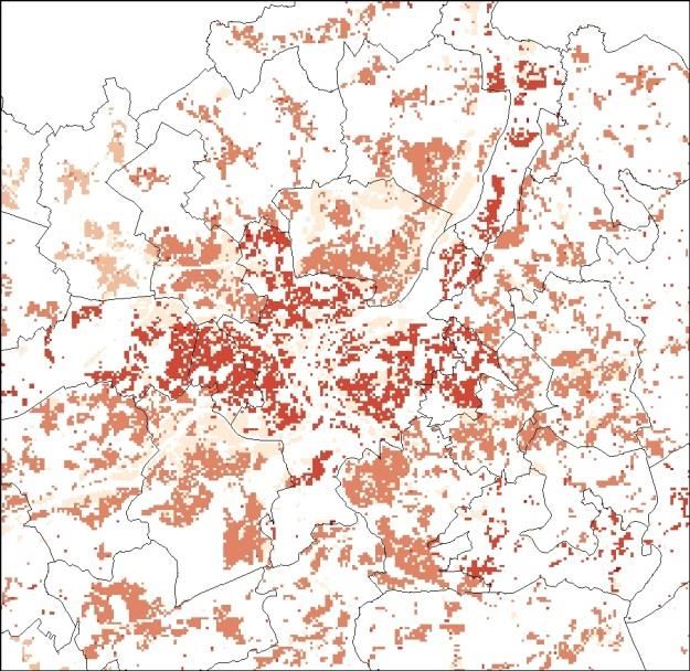
Figure 17 Growth of the residential area in the period 2008-2050 in the BAU (upper) en STOP (lower)
 scenario. In grey: existing residential cells, in red: newly developed residential cells by 2050

 18/08/2017 – v9 32

Figure 18 Residential growth in period 2008-2050 in hectares (upper) and in percentage (lower) for
 the BAU and STOP scenario

4.2. GENERAL TRENDS IN THE WALLOON REGION COMPARED TO FLANDERS

Since the SmartPop land-use model is inspired by the Flemish ‘RuimteModel Vlaanderen’, a
comparison between the results of both models can be drawn.

In both regions, a continuous trend of urbanisation is taking place. Figure 19 shows the daily
urbanisation rate in Flanders and Wallonia for a period in the past, according to cadastral
information, and for the period towards 2050 according to the model simulations.
In Flanders, the urbanisation trend is currently taking place at a rate of more or less 6ha /day. This is
already a decrease in comparison to the period 1985-1995 in which the built-up expansion occurred
at a growth rate of more than 10 ha/day. Since 2000 the growth rate has stabilised at a rate of more
or less 6 ha/day. In the Flemish Business-as-Usual scenario this slowly decreasing trend of the last 10
years is extrapolated towards 2050, resulting in a growth rate which goes down to more or less 2
ha/day by 2050. In the Walloon region, on the other hand, the current urbanisation rate is somewhat
lower (ca 3.5 ha/day). In a BAU-scenario for the Walloon region, this growth rate is also slowly
decreasing to around 1 ha/day by 2050. In other words, while the difference between Flanders and
the Walloon region is quite large currently, this difference will slowly decrease in a business-as-usual
development in both regions.
Moreover, in a scenario in which a zero-growth is implemented, the urban growth in the Walloon
region will even be at a larger rate than in Flanders. This is because the Flemish government wants to
implement a zero growth (betonstop) by 2040, while in the Walloon region, this zero growth or built-
up land will only by in place by 2050.

 18/08/2017 – v9 33