X-Ray Study of Variable Gamma-Ray Pulsar PSR J2021+4026
←
→
Page content transcription
If your browser does not render page correctly, please read the page content below
The Astrophysical Journal, 856:98 (11pp), 2018 April 1 https://doi.org/10.3847/1538-4357/aab202
© 2018. The American Astronomical Society. All rights reserved.
X-Ray Study of Variable Gamma-Ray Pulsar PSR J2021+4026
H. H. Wang1, J. Takata1 , C.-P. Hu2 , L. C. C. Lin3, and J. Zhao1
1
School of Physics, Huazhong University of Science and Technology, Wuhan 430074, People’s Republic of China; takata@hust.edu.cn
2
Department of Physics, The University of Hong Kong, Pokfulam Road, Hong Kong
3
Department of Physics, UNIST, Ulsan 44919, Republic of Korea
Received 2017 October 11; revised 2018 January 11; accepted 2018 January 31; published 2018 March 28
Abstract
PSRJ2021+4026 showed a sudden decrease in the gamma-ray emission at the glitch that occurred around 2011
October 16, and a relaxation of the flux to the pre-glitch state at around 2014 December. We report X-ray analysis
results of the data observed by XMM-Newton on 2015 December 20 in the post-relaxation state. To examine any
change in the X-ray emission, we compare the properties of the pulse profiles and spectra at the low gamma-ray
flux state and at the post-relaxation state. The phase-averaged spectra for both states can be well described by a
power-law component plus a blackbody component. The former is dominated by unpulsed emission and probably
originated from the pulsar wind nebula as reported by Hui et al. The emission property of the blackbody
component is consistent with the emission from the polar cap heated by the back-flow bombardment of the high-
energy electrons or positrons that were accelerated in the magnetosphere. We found no significant change in the
X-ray emission properties between two states. We suggest that the change of the X-ray luminosity is at an order of
∼4%, which is difficult to measure with the current observations. We model the observed X-ray light curve with
the heated polar cap emission, and we speculate that the observed large pulsed fraction is owing to asymmetric
magnetospheric structure.
Key words: methods: data analysis – pulsars: individual (J2021+4026) – stars: neutron – X-rays: stars
1. Introduction with (1) a decrease of flux (>100 MeV) by ∼18%,
from (8.33 ± 0.08)×10−10 erg cm−2 s−1 to (6.86 ± 0.13)×
A pulsar is a fast spinning and highly magnetized neutron
10−10 erg cm−2 s−1, (2) a significant change in the pulse profile
star, which is a condensed star with an averaged mass density
(>5σ), and (3) a marginal change in the gamma-ray spectrum
of ∼1014–15 gcm−3, and it is observable in radio to very high-
(200 pulsars4,5 (Abdo et al. 2013). the timing analysis of ∼8 year Fermi-LAT data, and they found
In particular, Fermi-LAT uncovered many new gamma-ray the relaxation at around 2014 December, where the spin-down
pulsars in the Cygnus region, and the most intriguing one rate and the gamma-ray emission returned to the state before
among them is PSR J2021+4026. PSR J2021+4026 is an the glitch. The pulse profile and spectrum after the relaxation
isolated pulsar that belongs to the Geminga-like pulsars are consistent with those before the glitch.
(lacking radio-quiet emission with certain detections of pulsed An unidentified X-ray source 2XMMJ202131.0+402645
detections in both the X-ray and gamma-ray bands; Lin 2016). had been investigated as a promising counterpart of PSR J2021
It is also known as the first variable gamma-ray pulsar seen by +4026 (Trepl et al. 2010; Weisskopf et al. 2011), and a deep
the Fermi-LAT. It is associated with the supernova remnant observation was done by XMM-Newton (ESA: XMM-Newton
G78.2+2.1 (Abdo et al. 2009b). This pulsar has a spin period SOC6) at MJD 56,028, when the pulsar stayed at the low
of P=265ms and a spin-down rate of Ṗ = 5.48 ´ 10-14 , gamma-ray flux state after the glitch. The detected spin
corresponding to a characteristic age of τc∼77 kyr, a surface frequency is consistent with the gamma-ray pulsation of PSR
dipole field of Bd∼4×10¹² G, and a spin-down power J2021+4026 at the same epoch, proving 2XMMJ202131.0
of Ė ~ 10 35 erg s-1. +402645 is indeed the counterpart of PSR J2021+4026 (Lin
Allafort et al. (2013) reported results of a detailed analysis on et al. 2013). The single broad pulse profile and the blackbody
the gamma-ray emission from PSR J2021+4026, and they spectrum with an effective temperature of kTB∼0.25 keV and
found a glitch around MJD55850 (2011 October 16) on a radius Reff∼300 m imply that the X-ray emission came from
timescale shorter than one week. This glitch increased the spin- the polar cap heated by the back-flow bombardment of the
down rate from ∣ f˙ ∣ = (7.8 0.1) ´ 10-13Hz s-1 to high-energy electrons or positrons that were accelerated in the
(8.1 ± 0.1)×10−13 Hz s−1. Moreover, the glitch accompanied magnetosphere.
Emission from the heated polar cap will be closely related to
4
https://confluence.slac.stanford.edu/display/GLAMCOG/Public+List the gamma-ray emission process. In the outer gap model, for
+of+LAT-Detected+Gamma-Ray+Pulsars
5 6
https://fermi.gsfc.nasa.gov/ssc/data/access/lat/fl8y/ “XMM-Newton Users Handbook,” Issue 2.15, 2017.
1The Astrophysical Journal, 856:98 (11pp), 2018 April 1 Wang et al.
Figure 1. About an eight-year evolution of the gamma-ray flux (top) and the spin-down rate (bottom). The epochs of the two X-ray observations are indicted in the top
panel. The figure is adopted from Zhao et al. (2017).
example, the pair-creation process inside the accelerator and the emproc/epproc tasks of the XMM-Newton Science
produces the electrons and positrons, and the electric field Analysis Software (XMMSAS, version 16.0.0). After filtering
along the magnetic field separates the pairs, and results in the the events, which are potentially contaminated, the effective
formation of the in-going and out-going particles (Zhang & exposures are 134 ks and 130 ks for MOS1 and MOS2, 94 ks
Cheng 1997). The created pairs inside the gap are accelerated for PN, respectively. A point source is significantly detected
to a Lorentz factor of >107 and emit the gamma-rays via the (>10σ) by XMMSAS task edetect_chain at the position of PSR
curvature radiation process. Half of the created pairs will return J2021+4026. To perform the spectral and timing analyses, we
to and heat up the polar cap region. In this model, the flux of extract EPIC data from circles with a radius of 20″ centered at
the observed X-ray emission will be proportional to the its nominal X-ray position (R.A., decl.)=(20h21m30 733,
gamma-ray flux. Hence, it is expected that the state change in +40°26′46 04) (J2000).
the spin-down rate/gamma-ray emission is also accompanied
with the change in the observed X-ray emission. In this paper,
we report the results of a new X-ray observation performed by 2.1. Timing Analysis
XMM-Newton in the post-relaxation state, and compare the
emission properties with the previous X-ray properties Our main purpose is to investigate the change in the pulsed
observed in the low gamma-ray flux state (Section 2). In X-ray emission before and after the relaxation occurred at
Section 3, we will discuss the X-ray light curve of the heated around 2014 December. Therefore, a timing analysis is crucial.
polar cap and the emission geometry. Following Lin et al. (2013), we divide the PN data into three
energy bands; 0.15–0.7 keV, 0.7–2.0 keV, and 2.0–12 keV. For
the timing analysis, the available photon number is 1399 counts
2. Data Analysis for 0.15–0.7 keV, 1170 counts for 0.7–2.0 keV, and 724 counts
We analyze the archive data taken by XMM-Newton on 2015 for 2.0–12 keV. The arrival times of all the selected events are
December 20 (MJD 57,376, Obs. ID: 0763850101, PI: barycentric-corrected with the aforementioned X-ray position
Razzano), which is about 3.7 years after the previous XMM- and the latest DE405 Earth ephemeris.
Newton observation performed in the low gamma-ray state (Lin In the analysis, the pulsation is significantly detected only in
et al. 2013), and about 1 year after the relaxation in 2014 0.7–2.0 keV energy bands, and no conclusive evidence of the
December (Figure 1). This new observation was performed pulsation is obtained in the energy bands of 0.15–0.7 keV and
with a total exposure of ∼140 ks. The MOS1/2 CCDs were 2.0–12 keV. Based on the Rayleigh test (Mardia 1972; Gibson
operated in the full-window mode (time resolution 2.6 s), and et al. 1982) applied for 0.7–2.0 keV observation, a significant
PN CCD was operated in the small-window mode (time peak is found at f=3.7688991(2)Hz with Z12 = 196, where
resolution 5.7 ms). Only PN data enables the timing analysis of we assessed the uncertainty with Equation 6(a) provided in
this pulsar. Event lists from the data are produced in the Leahy (1987), using total duration of ∼100 ks. In 0.15–0.7 keV
standard way using the most updated instrumental calibration and 2.0–12 keV energy bands, the X-ray pulsation is
2The Astrophysical Journal, 856:98 (11pp), 2018 April 1 Wang et al.
Figure 2. Energy dependent X-ray folded light curves of PSRJ2021+4026 in the energy bands 0.15–0.7 keV (upper), 0.7–2.0 keV (middle), and 2.0–12 keV
(bottom). Two cycles are presented for clarity. In the middle panel, the vertical solid and dashed lines define the on-pulse and off-pulse phase, respectively, and the
horizontal dashed line shows a background level determined by the nearby source-free region. We normalize the count so that the average intensity is unity, indicating
the background emission occupies about 50% of the 0.7–2.0 keV emission from the direction of the source.
Figure 3. Folded light curves of PSR J2021+4026 in 0.7–2.0 keV (thick histograms) and >0.1GeV (thin histograms) energy bands. Left panel: low gamma-ray flux
state. Right panel: post-relaxation state.
insignificant with Z12 ~ 5. This spin frequency is consistent dashed line) with a nearby source-free region, and we can find that
with that derived by the Fermi-LAT (Zhao et al. 2017). the background emission explains about 50% of the emission from
Figure 2 shows the folded light curves in three energy bands; the direction of the source and it explains the emission at the off-
0.15–0.7 keV (top), 0.7–2.0 keV (middle), and 2.0–12 keV pulse phase. It is expected, therefore, that the pulse profile after
(bottom). In the figure, the folded light curve in 0.7–2.0 keV subtracting the background has a large pulsed fraction, which is
bands shows a broad and single peak pulse profile. In Figure 3, defined by F=( fmax−fmin)/( fmax + fmin)×100% with fmax and
we compare the light curves in 0.7–2.0 keV energy bands in the fmin being the maximum and minimum count rates, respectively.
low gamma-ray flux state (right panel) and in the post-relaxation The large pulsed fraction (F ∼ 100%) can be used to constrain the
state (left panel). Within the current quality of the data, no emission geometry by modeling the light curve of the heated polar
significant difference can be seen in the two pulse profiles. cap emission (Section 3).
In the X-ray light curve of the 0.7–2.0 keV energy band (middle Lin et al. (2013) compared the pulse phases in X-ray and
panel of Figure 2), we determine a background level (horizontal gamma-ray bands in the low gamma-ray flux state, and found
3The Astrophysical Journal, 856:98 (11pp), 2018 April 1 Wang et al.
Table 1 states simultaneously using the XSPEC (version 12.9.1). Since
Ephemeris of PSR J2021+4026 the interstellar hydrogen is the main absorber of X-rays, we
Parameters expect that the hydrogen column density (NH) is not changed
by the state change. In the analysis, therefore, we tie the
R.A. 20h21m30 733
Decl. +40°26′46 04 column densities in the two data sets, and leave all other
Valid MJD range 57,283∼57,471 parameters free. First, we fit the data with the single-component
Pulse frequency, f (Hz) 3.7688994400(7) model, that is, a single power law (PL) or a single blackbody
First derivative of pulse frequency, f˙ (s-2) −7.707(4)×10−13 (BB) radiation model. We found that the single-component
Second derivative of pulsar frequency, f" (s−3) 6.0(9)×10−22 model cannot provide appropriate fits; for the power-law
Third derivative of pulsar frequency, f ⃛ (s−4) 2(9)×10−29 model, the best-fit power-law index is very large (Γ ∼ 4) with
Epoch zero of the timing solution (MJD) 57,377 χ2=162 for 121 degrees of freedom (dof), which is far
rms timing residual (μs) 1677.862 steeper than that (Γ ∼ 1.5) predicted by the synchrotron
radiation from the secondary electron/positron pairs (Cheng
& Zhang 1999). The blackbody model also provides an
that the X-ray peak lags the stronger gamma-ray peak (the unacceptable fit with χ2=205 for 121 dof.
second peak) and proceeds after the smaller peak (the first Since Lin et al. (2013) obtained a reasonable fit with the PL
peak). To investigate the phase relation between the X-ray and +BB model, we also apply the PL+BB model for the
gamma-ray pulses in the post-relaxation state, we extract the
simultaneous fitting. We found that the PL+BB model can
Fermi-LAT data of about a half year (MJD 57,283–57,471)
describe the data in the low gamma-ray flux state and the post-
centered at the epoch of the X-ray observation, and create local
ephemeris (Table 1). With the standard process for the data relaxation state simultaneously, and the best fitting parameters
reduction using the Fermi-Scinece tools v10r0p5 package (Zhao of the X-ray data in both states are consistent with each other
et al. 2017 for more details of PSR J2021+4026), we assign the within 1σ error (Table 2); the observed spectra are well fitted with
probability of each photon originating from the pulsar. After the photon index Γ∼1–1.3, the surface temperature of kTB∼
performing the gtbary task for barycentric time corrections to 0.25–0.3 keV and the effective radius of Reff∼250–300 m. The
photon arrival times, we convert the arrival time to the pulsar spin observed flux in the energy band of 0.2–12 keV is dominated by
phase using the local ephemeris created by Fermi-LAT data (i.e., the blackbody component. The result is consistent with that
Table 1). indicated in Lin et al. (2013), and the power-law component
Figure 3 summarizes the light curves of PSR J2021+4026 in probably came from the pulsar wind nebula (Hui et al. 2015).
the X-ray (thick histograms) and gamma-ray (thin histograms) Figure 5 shows the confidence contours on the plane determined
using the same ephemeris reported in Lin et al. (2013) for the by the photon index and the temperature. We can see in the figure
low gamma-ray flux state (left panel) and the ephemeris in that the distributions of the errors are very similar as well,
Table 1 for the post-relaxation state (right panel). As we can suggesting no significant evolution of the spectral properties.
see in the figure, the phase correlation between the X-ray peak
and the gamma-ray peak in the post-relaxation state is very
similar to that in the low gamma-ray flux state, that is, the 2.3. Spectrum of the Pulsed Component
X-ray peak lags the stronger gamma-ray peak (the second peak)
and proceeds after the smaller peak (the first peak). The cross- We analyze the data in the low gamma-ray flux state and in
correlation coefficient attains the maximum value at a phase lag the post-relaxation state, and we compare the spectra of the
of ∼−0.14 for both states. Hence, no significant change in the pulsed component for two states. According to Figure 2 of the
correlation of the X-ray and gamma-ray pulsations before and post-relaxation state, we define the phase intervals of 0.2–0.6
after the relaxation is found. and 0.7–1.0 as the “on-pulse” and “off-pulse” (i.e., DC level)
components, respectively. We also use the same intervals in the
light curves of the low gamma-ray flux state. The event files in
2.2. Spectral Analysis each phase are extracted using xronwin and xselect, and the
2.2.1. Phase-averaged Spectrum spectrum of the pulsed component is obtained by subtracting
the spectrum of “off-pulse” phase from that of the “on-pulse”
In order to further investigate the X-ray emission properties phase. Because of the limited photon counts, we grouped the
from this pulsar, we carry out the spectral analysis of all three
channels so as to archive the signal-to-noise ratio S/N=2 in
EPIC cameras (MOS1/2 and PN), and we compare with
each energy bin. The generated spectra (Figure 6) are fitted by
the previous results given in the low gamma-ray flux state. We
the single BB model, and its best-fit parameters (Table 3) are
generate the spectra of MOS1/2 and PN from photons in
the 0.15–12 keV energy bands within a radius of 20″ circle kTB∼0.26 keV and Reff∼250 m at d=1.5 kpc. The result in
centered at the source. The background spectra are generated low gamma-ray flux state is fully consistent with the result in
from a nearby region of the same size as the corresponding Hui et al. (2015). The single power-law model also provides an
CCD. The response files are generated by the XMMSAS tasks acceptable fit. However, the best-fit photon index is very large
rmfgen and arfgen. We group the channels so as to achieve the (Γ ∼ 3.8) with χ2=8.41 for 15 dof, again which is far steeper
signal-to-noise ratio S/N=3 in each energy bin. than the theoretical prediction (Γ ∼ 1.5). The two component
Figure 4 shows the phase-averaged spectrum in the post- (BB+PL) model fits the data with kTB∼0.19 keV, but the
relaxation state taken by all three cameras. To investigate any model cannot constrain the photon index. Based on our fitting
changes of the spectral properties in the low gamma-ray flux presented in Table 3, no significant change is found in the
state and the post-relaxation state, we fit the data in the two pulsed spectra before and after relaxation of the state.
4The Astrophysical Journal, 856:98 (11pp), 2018 April 1 Wang et al.
Figure 4. Phase-averaged spectrum of PSRJ2021+4026 in 0.5–10 keV. The observed spectra with the PN (green spectrum) and MOS1/2 detectors (black and red
spectra) are simultaneously fitted by an absorbed blackbody plus power-law model.
Table 2 2013; Hui et al. 2015), the observed X-ray emission likely
Parameters of the Phase-averaged Spectra Determined in the Low Gamma-Ray originated from the polar cap heated by the bombardment of the
Flux State (Middle Column) and in the Post-relaxation State (Third Column)
high-energy electrons or positrons that were accelerated in an
Parameters MJD56,028 MJD57,376 acceleration region.
NH(10 cm )
22 −2 +0.4
0.9-
Fermi-LAT found that the gamma-ray flux above the cutoff
Fluxbb (10−13 erg cm−2 s−1)a +1.4
1.4-
0.3
+1.5
1.6-
energy at around ∼3 GeV decays slower than a pure
Fluxp (10−14 erg cm−2 s−1)b
0.6
+1.3
3.5-
0.7
+1.4
4.7-1.0
exponential function (Abdo et al. 2013). This cutoff behavior
0.7
+0.03 +0.04 favors the emissions from the outer magnetosphere (e.g., Arons
kTB (kev) 0.21- 0.03 0.21- 0.04
+591 +622 1983 for the slot gap model, Cheng et al. 1986a, 1986b for the
Reff (m)c 272- 255 255- 245
+0.7 +0.9 outer gap model, and Spitkovsky 2006 for the current sheet),
Photon index 1.0- 1.3-
0.8 0.9
and it rules out the classical polar cap scenario (e.g., Daugherty
χ 2/dof 105.89/114
& Harding 1996), which predicted a super exponential cutoff
feature in the GeV spectrum because of the magnetic pair-creation
Notes.The uncertainties of each of the spectral parameters are assessed in 1σ
for four parameters of interest for the multi-component model.
process. In the outer gap model (Cheng et al. 1986a, 1986b; Zhang
a
Flux of the blackbody component in 0.2–12 keV. & Cheng 1997; Takata et al. 2010), for example, the luminosity of
b
Flux of the power-law component in 0.2–12 keV. the gamma-ray from the accelerated electrons/positrons and of the
c
Effective radius at d=1.5 kpc. heated polar cap are characterized by the so-called fractional gap
width, fgap, which is defined by the ratio of the angular size of the
gap thickness measured on the stellar surface to the angular size of
3. Discussion and Summary the polar cap (i.e., qp = RNS Rlc ). The electrodynamics of the
3.1. Emission from the Heated Polar Cap outer gap expects that the radiation power of the gamma-ray
emission is of the order of
We have compared the properties of the X-ray emission
observed at MJD56,028 in the low gamma-ray flux state and at L g ~ Igap ´ Vgap ~ fgap
3
Lsd , (1 )
MJD57,376 observed in the post-relaxation state. Although both
spin-down rate and gamma-ray flux observed at the two epochs where Igap and Vgap are the electric current and potential drop
are different, our measurements find no significant change in any along the magnetic field line, respectively. In the outer gap, they
of the X-ray emission properties. The blackbody radiations in both may be of the order of Igap ~ pfgap Bd RNS 3
(PRlc ) and Vgap =
states are measured with an effective radius Reff∼300 m at 2 3
d=1.5 kpc, which is comparable to the theoretical prediction of fgap Bd RNS (2Rlc2 ), respectively, where Bd denotes the surface
the polar cap size, Rpc∼RNS(RNS/Rlc)1/2∼280 m, where RNS= magnetic dipole field. The gamma-ray emission from PSRJ2021
106 cm is the neutron star radius, and Rlc=cP/2π is the light +4026 (Lsd ~ 1.2 ´ 10 35 erg s-1) is measured with a luminosity
cylinder radius that can be derived from the spin period (P) and of Lγ∼5×1034(d/1.5 kpc)2(ΔΩ/3radian) erg s−1, where ΔΩ is
the light speed (c). As proposed in the previous studies (Lin et al. the solid angle of the gamma-ray beam. The fraction gap
5The Astrophysical Journal, 856:98 (11pp), 2018 April 1 Wang et al.
Figure 5. 1σ, 2σ, and 3σ error contours of the spectral parameters for the low gamma-ray flux state (dash line) and post-relaxation state (solid line). The black and blue
cross symbols indicate the parameters providing the minimum χ2 for the low gamma-ray flux state and post-relaxation state, respectively.
thickness, therefore, is estimated as fgap∼0.75, indicating that a increased by δIc/Ic∼4%. If we estimate the fractional gap
large fraction of the spin-down power is converted into the high- thickness from fgap=(Lγ/Lsd)1/3, the observation implies that the
energy radiation. fractional gap thickness decreased by δfgap/fgap∼−8%. Since the
The electrons and positrons in the outer gap are separated by X-ray luminosity is proportional to fgapIc, the expected change in
the electric field parallel to the magnetic field line, and half of LX is found to be ∣dLX LX ∣ ~ ∣dIc Ic + dfgap fgap ∣ ~ 4%, which
the accelerated particles will be returned to the polar cap. The is smaller than the current uncertainty of our measurement
number of particles returned to the polar cap is of the order of (>10%). Hence it is difficult to measure the change of the X-ray
Igap emission before and after the relaxation with the current
N˙e ~ ~ 7 ´ 1029fgap P -2B12 s-1, (2 ) observations.
2e
where B12 is the surface magnetic field in units of 1012G.
3.2. X-Ray/Gamma-Ray Light Curve Model
Because of the curvature radiation process during the travel
from the inner boundary of the outer gap to the stellar surface, As we have discussed above, the X-ray emission likely
each return particle carries only 10.6P1/3 ergs onto the stellar originated from the heated polar cap region, and the GeV
surface (Halpern & Ruderman 1993; Zhang & Cheng 1997). gamma-ray may be produced in the outer magnetosphere. The
As a result, the luminosity of the X-rays from the heated polar X-ray peak leading the first peak in the gamma-ray pulse profile
cap region is estimated by will also be consistent with the GeV gamma-ray emission from
the outer magnetosphere (e.g., Romani & Yadigaroglu 1995).
LX ~ 10.6P1 3 erg · N˙e ~ 10 31fgap B12 P -5 3 erg s-1, (3 ) The gamma-ray emission from PSRJ2021+4026 is observed
with a double peak in the light curve separated by about a half-
which gives the order of LX∼1032 erg s−1 for PSRJ2021 spin phase. Trepl et al. (2010) interpreted the phase separation
+4026. Since the X-ray emission from PSRJ2021+4026 with the outer gap accelerator model and expected the viewing
likely originated from the polar cap heated by the back-flow angle of ∼90° measured from the rotation axis. Hui et al. (2015)
particles that were accelerated in the outer magnetosphere, it is assumed an orthogonal rotator with a single pole contribution to
fit the X-ray light curve. Since the previous studies did not
expected that the state change in the spin-down rate/gamma-ray
discuss in detail the phase relation between the gamma-ray pulse
emission accompanies the change in the heated polar cap emission. and X-ray pulse for PSRJ2021+4026, we compare the observed
In the low gamma-ray flux state, the spin-down rate was ∼4% X-ray/GeV light curves with the theoretical model.
higher than one in the pre-glitch and post-relaxation states. We Since the radius of the polar cap region of PSRJ2021+4026 is
speculate that the change in the magnitude of the global current of the order of 200–300 m, which is much smaller than the
caused the change in the spin-down rate at the glitch and at the neutron star size, we can safely ignore the size of the polar cap
relaxation, and that the current in the low gamma-ray flux state region, and assume the point-like hot spots at the magnetic poles.
6The Astrophysical Journal, 856:98 (11pp), 2018 April 1 Wang et al.
Figure 6. Pulsed spectrum of PSR J2021+4026 in the post-relaxation state. This spectrum is obtained by subtracting the data of the off-pulse phase from the on-pulse
phase and provides the best fit for a single blackbody model in the energy band of 0.2–7 keV. The lower panel demonstrates the χ2 fit statistic.
Table 3
where α and ζ are the angles of the magnetic axis and the line
Parameters of the Pulsed Spectra in the Low Gamma-Ray Flux State (Middle of sight measured from the spin axis.
Column) and in the Post-relaxation State (Third Column) We assume that the observed count at each spin phase in the
Parameter MJD56,028 MJD57,376
light curve is proportional to I0 (q ) cos q , where I0(θ) is the local
−2 −1 a +0.4
intensity. For the isotropic emission, I0(θ)=constant, the
Flux (10 erg cm
13
s ) 1.3-0.30.3 1.0-0.3 previous studies (e.g., Beloborodov 2002; Bogdanov 2016)
+0.04 +0.05
kTB (keV) 0.27- 0.03 0.27-0.04 demonstrated that the emissions from the two PCs, which are
+240 +258
Reff (m)b 234- 214-
168 163 equally heated up, make the pulse profile with a small pulsed
χ2/dof 17.13/17
fraction F∼10% (see also Figure 7). This is because the light
bending effect allows us to measure the emission from the
Notes.The hydrogen column density is fixed at NH=7×1021cm−2.
a
Flux in 0.2–12 keV.
backside of a neutron star and because the observer can almost
b
Effective radius at d=1.5 kpc. always see the emission from two poles. A neutron star
atmosphere model with a strong magnetic field has been
developed by the previous studies (e.g., Pavlov et al. 1994;
Zavlin et al. 1995; Ho & Lai 2001, 2003; Zane & Turolla 2006).
The theory including gravitational light bending for the hotspot
It is discussed that the neutron star atmosphere with a strong
emission on the neutron star surface has been developed in the
magnetic field makes the emission highly anisotropic, and the
previous studies (Pechenick et al. 1983; Beloborodov 2002;
Bogdanov et al. 2007; Bogdanov 2016). In this paper, we apply higher intensity emerges along the magnetic field. Zavlin et al.
an approximation relation (Beloborodov 2002; Bogdanov 2016), (1995) demonstrate that the atmosphere with a strong magnetic
field can generate the light curve with a larger pulsed fraction
cos q - Rs RNS and a shaper pulse width.
cos y ~ , (4 ) To compare the atmosphere-model light curve with the
1 - Rs RNS
observation of PSRJ2021+4026, we refer to the results of
Zavlin et al. (1995), who calculate the angular distribution, I(θ),
where ψ and θ are the escape direction and the local angle of the
with the pulsar parameters of kBTeff∼0.25 keV and Bd∼
emission direction, respectively. In addition Rs = 2GMNS c 2 ,
1.2×10¹² G. Since their temperature of the heated polar cap is
and MNS is the mass of the neutron star. Such a formula can be similar to that of PSRJ2021+4026 (kTeff ∼ 0.21 keV), we may
used for RNS/RS>2. In this paper, we present a result with expect that their results can represent the case of PSRJ2021
RNS/Rs that is ∼2.35 for typical MNS=1.4 Me and RNS= +4026. Pavlov et al. (1994) compare the calculated angular
10 km. The escape angle ψ is related to the spin phase as distributions of the intensity for the nonmagnetic case Bd=0
and the magnetic case Bd=1.18×10¹² G. From their results,
⎛ t⎞
cos y (t ) = sin a sin z cos ⎜2p ⎟ + cos a cos z , we may expect that a slight difference in the dipole magnetic
⎝ P⎠ field (Bd ∼ 4 × 10¹² G for PSR J2021+4026 comparing with
7The Astrophysical Journal, 856:98 (11pp), 2018 April 1 Wang et al.
Figure 7. Model light curves for the isotropic emission (I(θ)=constant) from both of the magnetic poles heated by the return current. The assumed magnetic
inclination angle α and the viewing angle ζ are indicated by the values in each panel. The light bending effect due to the neutron star gravity is taken into account with
RNS/Rs=2.35 (Beloborodov 2002; Bogdanov 2016).
Figure 8. Same as Figure 7, but the local intensity depends on local emission angle. The angular distribution is read from those of models 2 and 3 in Figure2(b) of
Zavlin et al. (1995).
Bs ∼ 1.2 × 10¹² G of Zavlin et al. 1995) does not significantly 0.7–2 keV energy bands, we read the angular distribution of
change the angular distribution. Zavlin et al. (1995) present the E=1.12 keV from Figure2(b) in Zavlin et al. (1995). Finally,
angular distributions for the photon energy E0=0.18, 1.12, Zavlin et al. (1995) also show that the angular distribution is
and 2.47 keV (Figure2 in Zavlin et al. 1995). Since the less dependent on the neutron star model, that is, RNS/Rs. In
significant pulsation of PSRJ2021+4026 is detected in this paper, therefore, we refer their result of RNS/Rs=2.418
8The Astrophysical Journal, 856:98 (11pp), 2018 April 1 Wang et al.
fraction. We speculate that the asymmetry could be introduced
by asymmetry of the magnetic field structure around the polar
caps. It is argued that near the stellar surface, the magnetic field
configuration is not dominated by a dipole field (Ruderman &
Cheng 1988; Ruderman 1991). Higher order multipole field
configuration is likely, and the strength of the multipole field
can be 1∼3 orders of magnitude larger than the global dipole
field. This could also affect the structure and magnetic pair-
creation process of the polar cap accelerator. For example,
Timokhin & Harding (2015) point out that the multiplicity of
the pair-creation cascade at the polar cap accelerator is sensitive
to the curvature and strength of the magnetic field. Moreover,
Harding & Muslimov (2011a, 2011b) argue that even a small
distortion of the dipole field and/or the offset of the polar cap
from the dipole axis can greatly enhance the accelerating
electric field and the resultant multiplicity of the pairs. It is
expected therefore that an asymmetry of the magnetic field of
Figure 9. Comparing between the model and observed (0.7–2 keV) light
curves. For the heated polar cap emission (dotted line), the angular distribution the two polar caps causes the asymmetry of the polar cap
of the intensity is approximated by Figure2(b) of Zavlin et al. (1995). The accelerators. If the polar cap accelerator supplies the return
background level (dashed line) is determined by the nearby source-free region. current to heat up the polar cap, the temperatures of the two
The model result is for α∼16° and ζ∼20°, which is determined by the polar caps could be different.
minimum chi-square.
The return particles can also be supplied by the accelerator
around the light cylinder, which is probably the emission site of
(model 2 in Zavlin et al. 1995). Figure 8 summarizes the model the observed GeV gamma-rays. For example, the outer gap
light curves for the different set of the inclination angle and accelerator is a possible region to supply the returning particles.
viewing angle. By comparing Figures 7 with 8, we can see that It has been argued that the outer gap structure is sensitively
the atmosphere with the magnetic field makes the light curve controlled by the electrons or positrons that enter into the gap
with a larger pulsed fraction (F ∼ 65%) and a shaper pulse from the outside along the magnetic field lines (Hirotani &
width, as demonstrated in the previous studies (Pavlov et al.
Shibata 2001; Takata et al. 2016). Moreover, the outer gap will
1994; Zavlin et al. 1995).
be quenched (or less luminous), if the particles with a super
Figure 9 compares the model light curve and the observed
Goldreich–Julian rate are supplied from the polar cap region to
0.7–1.2 keV light curve; in the model, we assume that 50% of
the outer gap accelerator. If the multipole fields in the south and
the total emission (solid line) is contributed by the background
north poles could be an asymmetric configuration, the
(dashed line), as indicated by the observed 0.7–2.0 keV
emission (Figure 2). We determine the inclination angle asymmetric pair-creation process at the two polar caps could
α∼16° and the viewing angle ζ ∼ 20° to minimize the chi- make one outer gap, connecting to one pole, less active than
square with the central points of the data. Within the current that connecting to the other pole.
simple treatment of the angular distribution, we find that The high-energy emission in the outer magnetosphere has been
although the size of the observational error is relatively large, discussed with the slot gap model (e.g., Arons 1983; Harding
the pulsed fraction predicted in the model light curve is smaller et al. 2008; Harding & Kalapotharakos 2015), the outer gap model
than that of the observation, as Figure 9 indicates. The pulsed (e.g., Cheng et al. 1986a, 1986b; Takata et al. 2011), and the
fraction indeed depends on many unknown parameters (e.g., current sheet of the force-free or dissipative pulsar magnetosphere
hotspot size, viewing geometry, beaming effect, and RNS/Rs). model (e.g., Spitkovsky 2006; Kalapotharakos et al. 2014, 2017;
For example, we can expect that the pulsed fraction decreases Cerutti & Beloborodov 2017). These models predict that a larger
with the increase of the hotspot size and with the decrease of viewing angle of ζ∼90° is preferred to explain the double peak
the ratio RNS/Rs. The pulsed fraction tends to increase with the structure of the GeV emission with the peak separation of ∼0.5
increase of the ratio RNS/Rs. The observed pulsed fraction phase for PSRJ2021+4026 (Takata et al. 2011; Kalapotharakos
(F ∼ 100%), however, can be explained by an unrealistically et al. 2014). With a larger viewing angle, on the other hand, the
large ratio RNS/Rs>5 with the current beaming effect. With a emission from two polar caps that are equally heated up will make
reasonable ratio RNS/Rs, a larger beaming effect will be a double peak structure in the X-ray light curve, as demonstrated
required to give rise to the observed pulsed fraction. A fine in Figures 7 and 8, which is inconsistent with the observation.
tuning of the parameters is required to explain the observed This also motivates us to speculate that one polar cap is less
X-ray light curve if two poles are equally heated up. active.
To obtain a more robust conclusion, it will be required to Figure 11 shows the model light curves of the X-ray from the
calculate the light curve integrated by the photon energy and heated polar cap and of the gamma-ray from the outer gap
with the magnetic field strength of PSRJ2021+4026, which accelerator by assuming that only one magnetic hemisphere is
will be done in subsequent studies. We may argue, on the other active, as illustrated by Figure 10; we assume α=60° and
hand, that if both poles are equally heated up by the return ζ=85°, and the outer gap in the north hemisphere (left panel)
currents, the resultant pulsed fraction would be smaller than or the south hemisphere (right panel) is active. As in Figure 8,
that observed for PSR J2021+4026, as Figure 9 indicates. we refer to the angular distribution of the local emission of the
Since it would not be necessary that the magnetosphere is polar cap from Zavlin et al. (1995). We find in the figure that
symmetric, the north and south poles could have different the single pole model can produce the single peak with a large
temperatures, and the resultant light curve has a large pulsed pulsed fraction, and it is consistent with the observation. To
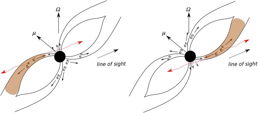
9The Astrophysical Journal, 856:98 (11pp), 2018 April 1 Wang et al. Figure 10. Possible geometry for PSRJ2021+4026. The charge separated pairs in the outer gap produce inwardly and outwardly propagating gamma-rays (red arrows), and the return particles heat up the polar cap region. The X-ray pulse profile indicates that only the single pole is heated up by the return current from the outer gap, and the outer gap in other hemisphere is quenched by the copious pairs from the polar cap region. The figure assumes ζ
The Astrophysical Journal, 856:98 (11pp), 2018 April 1                                                                                                   Wang et al.

                               References                                            Hui, C. Y., Seo, K. A., Lin, L. C. C., et al. 2015, ApJ, 799, 76
                                                                                     Kalapotharakos, C., Harding, A. K., & Kazanas, D. 2014, ApJ, 793, 97
Abdo, A. A., Ackermann, M., Ajello, M., et al. 2009a, APh, 32, 193                   Kalapotharakos, C., Harding, A. K., Kazanas, D., & Brambilla, G. 2017, ApJ,
Abdo, A. A., Ackermann, M., Ajello, M., et al. 2009b, ApJS, 183, 46                     842, 80
Abdo, A. A., Ajello, M., Allafort, A., et al. 2013, ApJS, 208, 17                    Leahy, D. A. 1987, A&A, 180, 275
Ackermann, M., Ajello, M., Albert, A., et al. 2012, ApJS, 203, 4                     Lin, L. C. C. 2016, JASS, 33, 147
Allafort, A., Baldini, L., Ballet, J., et al. 2013, ApJL, 777, L2                    Lin, L. C. C., Hu, C. Y., Hu, C. P., et al. 2013, ApJL, 770, L9
Arons, J. 1983, ApJ, 266, 215                                                        Mardia, K. V. 1972, Statistics of Direction Data (New York: Academic)
Atwood, W. B., Abdo, A. A., Ackermann, M., et al. 2009, ApJ, 697, 1071               Ng, C. W., Takata, J., Cheng, K. S., et al. 2016, ApJ, 825, 18
Beloborodov, A. M. 2002, ApJL, 566, 85                                               Pavlov, G. G., Shibanov, Y. A., Ventura, J., & Zavlin, V. E. 1994, A&A, 289, 837
Bogdanov, S. 2016, EPJA, 52, 37                                                      Pechenick, K. R., Ftaclas, C., & Cohen, J. M. 1983, ApJ, 274, 846
Bogdanov, S., Rybicki, G. B., & Grindlay, J. E. 2007, ApJ, 670, 668                  Romani, R. W., & Yadigaroglu, I.-A. 1995, ApJ, 438, 314
Cerutti, B., & Beloborodov, A. M. 2017, SSRv, 207, 111                               Ruderman, M. 1991, ApJ, 366, 261
Cheng, K. S., Ho, C., & Ruderman, M. 1986a, ApJ, 300, 500                            Ruderman, M., & Cheng, K. S. 1988, ApJ, 335, 306
Cheng, K. S., Ho, C., & Ruderman, M. 1986b, ApJ, 300, 522                            Spitkovsky, A. 2006, ApJL, 648, 51
Cheng, K. S., & Zhang, L. 1999, ApJ, 515, 337                                        Takata, J., Ng, C. W., & Cheng, K. S. 2016, MNRAS, 455, 4249
Daugherty, J. K., & Harding, A. K. 1996, ApJ, 458, 278                               Takata, J., Wang, Y., & Cheng, K. S. 2010, ApJ, 715, 1318
Gibson, A. I., Harrison, A. B., Kirkman, I. W., et al. 1982, Natur, 296, 833         Takata, J., Wang, Y., & Cheng, K. S. 2011, MNRAS, 415, 1827
Halpern, J. P., & Ruderman, M. 1993, ApJ, 415, 286                                   Timokhin, A. N., & Harding, A. K. 2015, ApJ, 810, 144
Harding, A. K., & Kalapotharakos, C. 2015, ApJ, 811, 63                              Trepl, L., Hui, C. Y., Cheng, K. S., et al. 2010, MNRAS, 405, 1339
Harding, A. K., & Muslimov, A. G. 2011a, ApJL, 726, 10                               Wang, Y., Takata, J., & Cheng, K. S. 2010, ApJ, 720, 178
Harding, A. K., & Muslimov, A. G. 2011b, ApJ, 743, 181                               Weisskopf, M. C., Romani, R. W., Razzano, M., et al. 2011, ApJ, 743, 74
Harding, A. K., Stern, J. V., Dyks, J., & Frackowiak, M. 2008, ApJ, 680, 1378        Zane, S., & Turolla, R. 2006, MNRAS, 366, 727
Hirotani, K., & Shibata, S. 2001, ApJ, 558, 216                                      Zavlin, V. E., Shibanov, Y. A., & Pavlov, G. G. 1995, AstL, 21, 149
Ho, W. C. G., & Lai, D. 2001, MNRAS, 327, 1081                                       Zhang, L., & Cheng, K. S. 1997, ApJ, 480, 370
Ho, W. C. G., & Lai, D. 2003, MNRAS, 338, 233                                        Zhao, J., Ng, C. W., Lin, L. C. C., et al. 2017, ApJ, 842, 53

                                                                                11
You can also read