Xilinx Software Development Kit (SDK) User Guide - System Performance Analysis UG1145 (v2018.3) December 05, 2018
←
→
Page content transcription
If your browser does not render page correctly, please read the page content below
Xilinx Software
Development Kit (SDK)
User Guide

System Performance Analysis

UG1145 (v2019.1) May 22, 2019
UG1145 (v2018.3) December 05, 2018
Revision History
05/22/2019: Released
The following        with Vivado®
              table shows          Design
                           the revision    Suite for
                                        history  2019.1
                                                     thiswithout changes from 2018.3.
                                                         document.

                    Section                                              Revision
                                       12/05/2018 Version 2018.3
General updates                                   Minor editorial changes.
                                       06/14/2016 Version 2016.2
General updates                                   Minor editorial changes.

System Performance Analysis                                                         Send Feedback
                                                                                                    2
UG1145 (v2019.1)
        (v2018.3)May 22, 2019
                 December   05, 2018        www.xilinx.com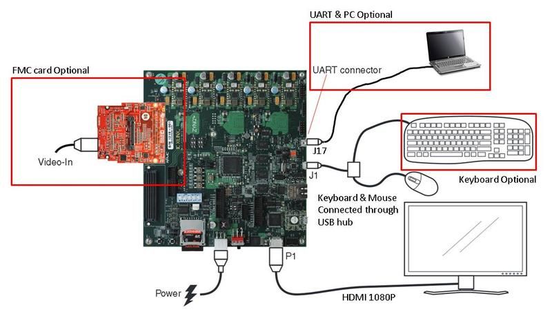
Table of Contents
          Revision History . . . . . . . . . . . . . . . . . . . . . . . . . . . . . . . . . . . . . . . . . . . . . . . . . . . . . . . . . . . . . . . . . . . . 2

       Chapter 1: Introduction
          SPA Toolbox . . . . . . . . . . . . . . . . . . . . . . . . . . . . . . . . . . . . . . . . . . . . . . . . . . . . . . . . . . . . . . . . . . . . . .   5
          Performance Analysis Flow . . . . . . . . . . . . . . . . . . . . . . . . . . . . . . . . . . . . . . . . . . . . . . . . . . . . . . . . . .             7
          Requirements . . . . . . . . . . . . . . . . . . . . . . . . . . . . . . . . . . . . . . . . . . . . . . . . . . . . . . . . . . . . . . . . . . . . .    9
          Additional Resources . . . . . . . . . . . . . . . . . . . . . . . . . . . . . . . . . . . . . . . . . . . . . . . . . . . . . . . . . . . . . . .        9

       Chapter 2: Background

       Chapter 3: System Performance Modeling Project
          SPM Software. . . . . . . . . . . . . . . . . . . . . . . . . . . . . . . . . . . . . . . . . . . . . . . . . . . . . . . . . . . . . . . . . . . . 15
          SPM Hardware . . . . . . . . . . . . . . . . . . . . . . . . . . . . . . . . . . . . . . . . . . . . . . . . . . . . . . . . . . . . . . . . . . . 18

       Chapter 4: Monitor Framework
          PL Profile Counters. . . . . . . . . . . . . . . . . . . . . . . . . . . . . . . . . . . . . . . . . . . . . . . . . . . . . . . . . . . . . . . . 22
          PS Profile Counters . . . . . . . . . . . . . . . . . . . . . . . . . . . . . . . . . . . . . . . . . . . . . . . . . . . . . . . . . . . . . . . 23
          Host-Target Communication . . . . . . . . . . . . . . . . . . . . . . . . . . . . . . . . . . . . . . . . . . . . . . . . . . . . . . . . 24

       Chapter 5: Getting Started with SPM
          ATG Configuration . . . . . . . . . . . . . . . . . . . . . . . . . . . . . . . . . . . . . . . . . . . . . . . . . . . . . . . . . . . . . . . . 26
          Performance Analysis Perspective . . . . . . . . . . . . . . . . . . . . . . . . . . . . . . . . . . . . . . . . . . . . . . . . . . . 27

       Chapter 6: Evaluating Software Performance
          Performance Monitoring. . . . . . . . . . . . . . . . . . . . . . . . . . . . . . . . . . . . . . . . . . . . . . . . . . . . . . . . . . . 30
          Visualizing Performance Improvements . . . . . . . . . . . . . . . . . . . . . . . . . . . . . . . . . . . . . . . . . . . . . . 33

       Chapter 7: Evaluating High-Performance Ports
          HD Video Traffic . . . . . . . . . . . . . . . . . . . . . . . . . . . . . . . . . . . . . . . . . . . . . . . . . . . . . . . . . . . . . . . . . . 37
          High-Bandwidth Traffic . . . . . . . . . . . . . . . . . . . . . . . . . . . . . . . . . . . . . . . . . . . . . . . . . . . . . . . . . . . . 39

       Chapter 8: Evaluating DDR Controller Settings
          Default DDRC Settings . . . . . . . . . . . . . . . . . . . . . . . . . . . . . . . . . . . . . . . . . . . . . . . . . . . . . . . . . . . . . 46

System Performance Analysis                                                                                                    Send Feedback
                                                                                                                                                                    3
UG1145 (v2019.1)
        (v2018.3)May 22, 2019
                 December   05, 2018                             www.xilinx.com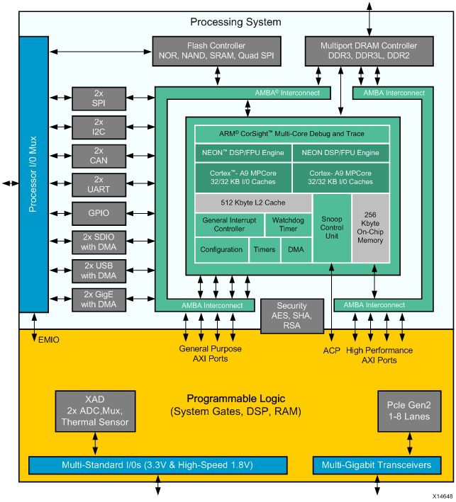
Modified DDRC Settings . . . . . . . . . . . . . . . . . . . . . . . . . . . . . . . . . . . . . . . . . . . . . . . . . . . . . . . . . . . 47
          Utilizing On-Chip Memory . . . . . . . . . . . . . . . . . . . . . . . . . . . . . . . . . . . . . . . . . . . . . . . . . . . . . . . . . . 49

       Chapter 9: Evaluating Memory Hierarchy and the ACP
          Assess Memory Performance . . . . . . . . . . . . . . . . . . . . . . . . . . . . . . . . . . . . . . . . . . . . . . . . . . . . . . . 51
          Data Size and Locality . . . . . . . . . . . . . . . . . . . . . . . . . . . . . . . . . . . . . . . . . . . . . . . . . . . . . . . . . . . . . 54
          Shared L2 Cache . . . . . . . . . . . . . . . . . . . . . . . . . . . . . . . . . . . . . . . . . . . . . . . . . . . . . . . . . . . . . . . . . . 55

       Chapter 10: Working with a Custom Target
          Instrumenting Software . . . . . . . . . . . . . . . . . . . . . . . . . . . . . . . . . . . . . . . . . . . . . . . . . . . . . . . . . . . 60
          Instrumenting Hardware . . . . . . . . . . . . . . . . . . . . . . . . . . . . . . . . . . . . . . . . . . . . . . . . . . . . . . . . . . . 61
          Monitoring a Custom Target . . . . . . . . . . . . . . . . . . . . . . . . . . . . . . . . . . . . . . . . . . . . . . . . . . . . . . . . 62

       Chapter 11: End-To-End Performance Analysis
          Assess Requirements . . . . . . . . . . . . . . . . . . . . . . . . . . . . . . . . . . . . . . . . . . . . . . . . . . . . . . . . . . . . . .          65
          Model Design . . . . . . . . . . . . . . . . . . . . . . . . . . . . . . . . . . . . . . . . . . . . . . . . . . . . . . . . . . . . . . . . . . . .     66
          Performance Validation. . . . . . . . . . . . . . . . . . . . . . . . . . . . . . . . . . . . . . . . . . . . . . . . . . . . . . . . . . . .            69
          In-Depth Analysis . . . . . . . . . . . . . . . . . . . . . . . . . . . . . . . . . . . . . . . . . . . . . . . . . . . . . . . . . . . . . . . . .      72

       Appendix A: Performance Checklist

       Appendix B: Additional Resources and Legal Notices
          Xilinx Resources . . . . . . . . . . . . . . . . . . . . . . . . . . . . . . . . . . . . . . . . . . . . . . . . . . . . . . . . . . . . . . . . . .     77
          Solution Centers. . . . . . . . . . . . . . . . . . . . . . . . . . . . . . . . . . . . . . . . . . . . . . . . . . . . . . . . . . . . . . . . . .      77
          Documentation Navigator and Design Hubs . . . . . . . . . . . . . . . . . . . . . . . . . . . . . . . . . . . . . . . . . . .                            77
          References . . . . . . . . . . . . . . . . . . . . . . . . . . . . . . . . . . . . . . . . . . . . . . . . . . . . . . . . . . . . . . . . . . . . . .   78
          Training Resources. . . . . . . . . . . . . . . . . . . . . . . . . . . . . . . . . . . . . . . . . . . . . . . . . . . . . . . . . . . . . . . .        79
          Please Read: Important Legal Notices . . . . . . . . . . . . . . . . . . . . . . . . . . . . . . . . . . . . . . . . . . . . . . . .                     79

System Performance Analysis                                                                                                     Send Feedback
                                                                                                                                                                   4
UG1145 (v2019.1)
        (v2018.3)May 22, 2019
                 December   05, 2018                              www.xilinx.com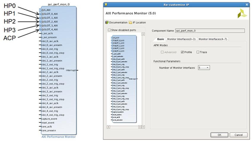
Chapter 1

Introduction
       The Xilinx® Zynq®-7000 SoC device family integrates a dual-core Arm® Cortex™-A9
       MPCore™ Processing System (PS) with Xilinx 7 series Programmable Logic (PL) in 28nm
       technology. The PS and PL are connected through standard Arm AMBA™ AXI interfaces
       designed for performance and system integration. This style of SoC is new to the industry,
       and therefore requires novel performance analysis and benchmarking techniques to
       provide you with a clear understanding of system performance. It is critical to understand
       the Zynq-7000 SoC architecture so that you can utilize its full potential and differentiate
       your products in the marketplace.

       SPA Toolbox
       To address the need for performance analysis and benchmarking techniques, the Xilinx
       Software Development Kit (SDK) has been enhanced with a System Performance Analysis
       (SPA) toolbox to provide early exploration of hardware and software systems. Specifically, a
       Zynq-7000 SoC designer is presented with insights into both the PS and the PL to
       understand the interactions across such a complex, heterogeneous system. You can observe
       system performance at critical stages of a design flow, enabling you to refine the
       performance of your system.

System Performance Analysis                                                  Send Feedback
                                                                                                  5
UG1145 (v2019.1)
        (v2018.3)May 22, 2019
                 December   05, 2018      www.xilinx.com
Chapter 1: Introduction

       X-Ref Target - Figure 1-1

                                   Figure 1-1:   Xilinx SDK Features Including the System Performance Analysis Toolbox

       Figure 1-1 shows how the SPA toolbox fits into the feature set of SDK. Other important
       features of SDK include software profiling tools, a system debugger, and supporting drivers
       and libraries. The SPA toolbox contains a monitor framework, user interface, and
       visualizations that are common for two important use models: an early exploration
       environment called System Performance Modeling (SPM) and the monitoring and analysis
       of your own designs. This common toolbox can be used for performance validation to
       ensure consistent and expected performance throughout the design process.

       SPM is a unique feature of SDK that enables complex performance modeling even before
       design work has started. SPM is executed in actual target hardware and includes a highly
       configurable, fixed bitstream containing five AXI traffic generators. These traffic generators
       are configurable cores used by SDK to model PL traffic activity. Software applications can
       also be run simultaneously in the processing system, and you can specify system
       configuration parameters.

System Performance Analysis                                                                          Send Feedback
                                                                                                                          6
UG1145 (v2019.1)
        (v2018.3)May 22, 2019
                 December   05, 2018                              www.xilinx.com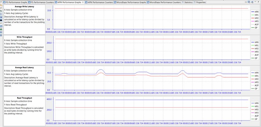
Chapter 1: Introduction

       Performance Analysis Flow
       Using the SPM design, SDK enables you to achieve an end-to-end performance analysis
       flow. This flow allows you to model the traffic of your estimated design and then validate
       the performance using your actual design.
       X-Ref Target - Figure 1-2

                                            Figure 1-2:   End-to-End Performance Analysis Flow

       As shown in Figure 1-2, this is a four-step process that includes:

       Assess Requirements – You first estimate the AXI traffic requirements of your design,
       including data throughputs at the PS-PL interfaces of the target system.

       Model Design – Based on these traffic requirements, you then use SPM to model your
       design. Since actual target hardware is used, real-time clock rates are achieved. This
       provides improved run-times over other modeling environments, as well as increased
       accuracy because real system activity is being monitored.

       Performance Validation – As you develop your design, you can validate the performance
       results by monitoring and visualizing your actual design.

       In-Depth Analysis - The SDK performance tools also enable a deep-dive analysis into your
       design to evaluate design options and gauge the impact of design improvements.

       There are multiple benefits to achieving such an end-to-end performance analysis flow,
       including:

       •                   Reduce risk for success – Achieving the desired latencies and throughputs with the
                           SPM-based model can provide a much stronger assurance that the final design will
                           achieve the same performance. While certainly not a guarantee, you can have
                           confidence that Zynq-7000 SoC can meet your performance goals.
       •                   Design Improvements – Running traffic scenarios using SPM will provide valuable
                           insights into system performance (for example, latencies) that will help you in your
                           actual design work.
       •                   What-If Scenarios – Since the SPM is a highly-configurable model, you can use it to try
                           variations of capabilities, features, and architectures.

       This guide describes the technical details of this performance analysis toolbox, as well as a
       methodology to appreciate its usefulness and depth. Note that this toolbox informs you as much
       about the capabilities of the target platform as it does about the particulars of a design.

System Performance Analysis                                                                  Send Feedback
                                                                                                                  7
UG1145 (v2019.1)
        (v2018.3)May 22, 2019
                 December   05, 2018                       www.xilinx.com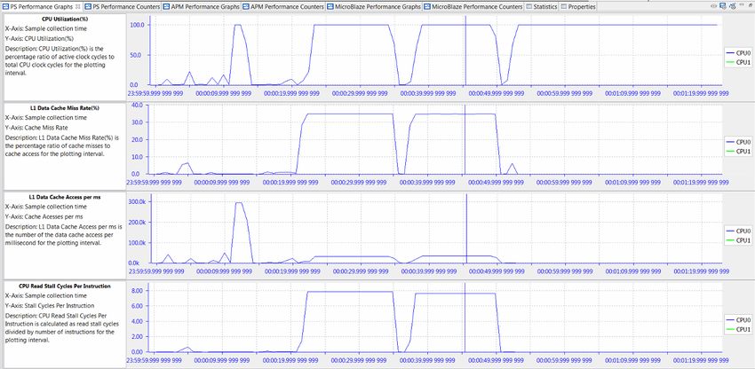
Chapter 1: Introduction

       Consequently, this guide is intended to highlight various features of the Zynq-7000 SoC, as well
       as how SDK can assist you in maximizing its capabilities. After reading this guide, you should be
       able to:

       •   Use the SPM design to analyze a software application and model hardware traffic
       •   Better understand the Zynq-7000 SoC platform and its proficiency
       •   Recognize the uses and capabilities of the PS-PL interfaces on the Zynq-7000 SoC
       •   Leverage the memory hierarchy (including the L1 and L2 data caches and DDR) to
           achieve the best system performance
       •   Model a design using SPM and follow up with performance validation of the actual
           design

       Specific examples are used to provide detailed results and analysis. This guide also
       describes how you can obtain similar results in SDK. The goals of this guide are such that
       you can extrapolate these techniques to model and analyze your own designs.

       The next four chapters provide an overview of the SPA toolbox:

       •   Chapter 2, Background outlines system performance and defines why it is important.
       •   Chapter 3, System Performance Modeling Project describes the contents of the SPM
           project.
       •   Chapter 4, Monitor Framework defines the monitoring infrastructure used by the SDK
           tool.
       •   Chapter 5, Getting Started with SPM provides the necessary steps to get up and
           running with the SPM design.

       The next set of chapters provides in-depth exploration into using the SPM design:

       •   Chapter 6, Evaluating Software Performance begins by running a software executable
           that comes with the SPM project.
       •   Chapter 7, Evaluating High-Performance Ports then introduces traffic on the
           High-Performance (HP) ports while running the same software
       •   Chapter 8, Evaluating DDR Controller Settings describes how to change DDR controller
           (DDRC) settings and analyze their impact on the HP port traffic.
       •   Chapter 9, Evaluating Memory Hierarchy and the ACP evaluates bandwidth and latency
           from the memory hierarchy, and then introduces traffic on the Accelerator Coherency
           Port (ACP) to investigate its impact on that performance.

       Additionally, two chapters are devoted to running performance analysis on your designs:

       •   Chapter 10, Working with a Custom Target defines some steps and requirements to
           instrumenting and monitoring your design.

System Performance Analysis                                                      Send Feedback
                                                                                                       8
UG1145 (v2019.1)
        (v2018.3)May 22, 2019
                 December   05, 2018        www.xilinx.com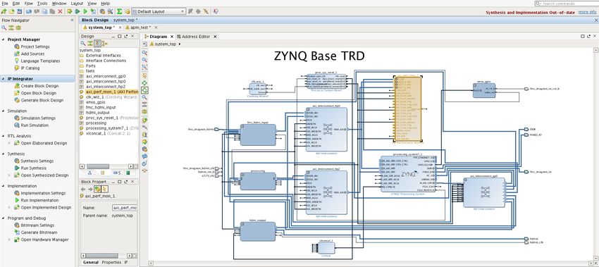
Chapter 1: Introduction

       •   Chapter 11, End-To-End Performance Analysis describes the full cycle of performance
           analysis as described in Figure 1-2.

       Finally, the key performance recommendations mentioned throughout this guide are
       summarized in Appendix A, Performance Checklist.

       Requirements
       If you would like to reproduce any of the results shown and discussed in this guide, the
       requirements include the following:

       1. Software
           a. Xilinx Software Development Kit (SDK) 2015.1
           b. Optional: USB-UART drivers from Silicon Labs
       2. Hardware
           a. Xilinx ZC702 evaluation board with the XC7Z020 CLG484-1 part
           b. AC power adapter (12 VDC)
           c. Xilinx programming cable; either platform cable or Digilent USB cable
           d. Optional: USB Type-A to USB Mini-B cable (for UART communications)
           e. Optional: Zynq-7000 SoC ZC702 Base Targeted Reference Design (UG925) [Ref 3].

       Additional Resources
       For a description of SDK and links to other guides, refer to the Xilinx SDK home page:

       https://www.xilinx.com/tools/sdk.htm

       Zynq-7000 SoC documentation, including the Zynq-7000 SoC Technical Reference Manual
       (UG585) [Ref 1], can be found here:

       https://www.xilinx.com/products/silicon-devices/soc/zynq-7000/index.htm

System Performance Analysis                                                 Send Feedback
                                                                                                  9
UG1145 (v2019.1)
        (v2018.3)May 22, 2019
                 December   05, 2018      www.xilinx.com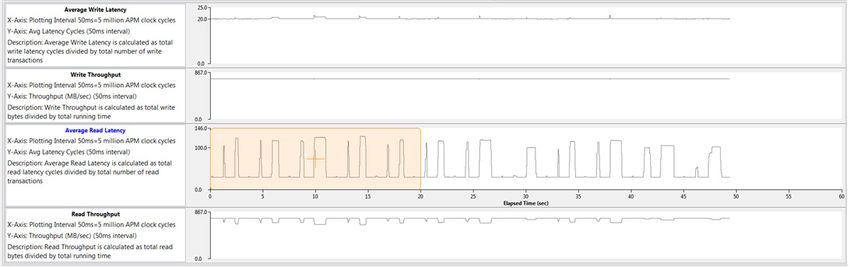
Chapter 2

Background
       Targeting a design to the Zynq®-7000 SoC can be facilitated if you are aware of the
       numerous system resources and their capabilities. After you become acquainted with the
       device, then you can decide how to map your functionality onto those resources and
       optimize the performance of your design.
       X-Ref Target - Figure 2-1

                                   Figure 2-1:    Block Diagram of Zynq-7000 SoC

System Performance Analysis                                                        Send Feedback
                                                                                                   10
UG1145 (v2019.1)
        (v2018.3)May 22, 2019
                 December   05, 2018             www.xilinx.com
Chapter 2: Background
Figure 2-1 shows the block diagram of the Zynq-7000 SoC. The Processing System (PS)
includes two Arm Cortex-A9 cores, a 512 KB L2 cache, a 256 KB on-chip memory, and a
number of peripherals and controllers.
The PL includes configurable system gates, DSPs, and block memories. There are three
types of interfaces between the PS and PL:
• General Purpose (GP) AXI Ports: control ports connected directly to the slave
interconnect
• Accelerator Coherency Port (ACP): low-latency access to PL masters, with optional
coherency with L1 and L2 cache
• High-Performance (HP) AXI Ports: PL bus masters with high bandwidth datapaths to the
DDR and OCM memories
These interfaces serve a variety of purposes for communication between the PS, the
Programmable Logic (PL), and any external memory (for example, DDR SDRAM or simply
DDR).
System Performance Analysis Send Feedback
11
UG1145 (v2019.1)
(v2018.3)May 22, 2019
December 05, 2018 www.xilinx.comChapter 2: Background
Flash Controller
NOR, NAND, SRAM, Quad SPI DDR Memory Controller
2x AMBA© Interconnect Interconnect
SPI
2x
I2C Arm© CorSight™ Multi-Core Debug and Trace
Processor I/0 Mux
2x NEON™ DSP/FPU Engine NEON DSP/FPU Engine
CAN
Cortex™- A9 MPCore Cortex- A9 MPCore
2x 32/32 KB I/0 Caches 32/32 KB I/0 Caches
UART
512 Kbyte L2 Cache
GPIO 256
General Interrupt Watchdog Snoop
Kbyte
Controller Timer Control
On-Chip
2x SDIO Unit
Memory
with DMA Configuration Timers DMA
2x USB
with DMA
2x GigE
with DMA AMBA Interconnect AMBA Interconnect
Security
AES, SHA, RSA
EMIO
General Purpose ACP High Performance
AXI Ports AXI Ports
XAD Programmable Logic
Pcle Gen2
2x ADC,Mux, (System Gates, DSP, RAM) 1-8 Lanes
Thermal Sensor
Multi-Standard I/0s (3.3V & High-Speed 1.8V) Multi-Gigabit Transceivers
X-Ref Target - Figure 2-2
Figure 2-2: Zynq-7000 SoC Block Diagram with Shared Resources Highlighted
Figure 2-2 highlights the shared resources in the Zynq-7000 SoC block diagram. A design
that fully utilizes all of the capabilities of this SoC requires multiple channels of
high-bandwidth communication. All of this traffic in the system inevitably involves shared
resources. In a poorly designed system this could lead to multiple points of contention
across the L2 cache, the DDR memory controller, and the high-speed interconnects. To
optimize the performance of a design that fully utilizes all of these resources, a designer
requires observability into multiple areas of such a system. Improvements can then be made
through code changes, design connectivity, or system settings.
System Performance Analysis Send Feedback
12
UG1145 (v2019.1)
(v2018.3)May 22, 2019
December 05, 2018 www.xilinx.comChapter 2: Background
An excellent example is the L2 cache. Because the ACP shares the L2 cache with the
Cortex-A9 CPUs, high-throughput traffic from either the ACP or the processors has the
potential to impact the performance of the other. While this effect can be anticipated,
understanding the nature and extent of this impact can be difficult.
This is where the SDK performance capabilities can be exploited. SDK provides the
visualizations to better understand this impact as well as SPM: an exploratory, early design
environment. Tables and real-time graphs are provided to visualize PS and PL performance
metrics on a common timeline. This provides much needed insight into when and where
things occur to quickly isolate any potential issues. Furthermore, the same performance
metrics are calculated for the SPM design as well as your own design, therefore providing
early performance exploration as well as consistent results across a design flow.
Before you begin using the performance tools and analyzing performance results, it is
important to understand what design is being used and what is being measured. The next
chapters summarize the SPM design and the performance monitor framework used by SDK.
System Performance Analysis Send Feedback
13
UG1145 (v2019.1)
(v2018.3)May 22, 2019
December 05, 2018 www.xilinx.comChapter 3
System Performance Modeling Project
Xilinx® Software Development Kit (SDK) is delivered with a predefined project that enables
System Performance Modeling (SPM) and helps enable performance analysis at an early
design stage. The SPM project contains both software executable and a post-bitstream,
configurable hardware system. The SPM serves multiple purposes, including the following:
• Target Evaluation – Gain a better understanding of the target platform with minimal
hardware design knowledge or experience. A complex SoC such as the Zynq®-7000
SoC can be characterized and evaluated, enabling critical partitioning trade-offs
between the Arm Cortex-A9s and the programmable logic. Most importantly, this
evaluation can be done independently of the progression or completion of a design.
You can always decide to gain a better understanding of your target platform.
• Perform Stress Tests – Identify and exercise the various points of contention in the
system. An excellent way of understanding a target platform is to evaluate the limits of
its capabilities.
• Performance Evaluation – Model the traffic of a design. Once the target platform is
understood, specifics of a design can be entered as traffic scenarios, and SPM can be
used to evaluate architectural options.
• Performance Validation – Instrument the final design and confirm results with the initial
model. The same monitoring used in the SPM design can also be added to your design
(see Instrumenting Hardware, page 61), providing a validation of the modeled
performance results.
System Performance Analysis Send Feedback
14
UG1145 (v2019.1)
(v2018.3)May 22, 2019
December 05, 2018 www.xilinx.comChapter 3: System Performance Modeling Project
X-Ref Target - Figure 3-1
Figure 3-1: SPM Project Files in SDK
Figure 3-1 lists the files contained in the predefined SPM project. It contains predefined
traffic configurations, two pre-compiled software executables, and many system definition
files. The system definition files include Processing System 7 (PS7) initialization files, a
Vivado® Design Suite Tcl file that creates the design definition in Vivado IP integrator, and
a bitstream containing a predefined Programmable Logic (PL) design.
SPM Software
The SPM project contains two pre-compiled software executables:
• A collection of benchmarks called the Bristol/Embecosm Embedded Energy Benchmark
Suite (BEEBS)
• Memory stride benchmarks designed specifically to test memory bandwidth and
latency
System Performance Analysis Send Feedback
15
UG1145 (v2019.1)
(v2018.3)May 22, 2019
December 05, 2018 www.xilinx.comChapter 3: System Performance Modeling Project
BEEBS Benchmarks
The BEEBS program comprises a sequence of eight diverse benchmarks. As shown in
Table 3-1, this suite contains algorithms originally contained as part of various well-known
benchmark suites such as MiBench, WCET, and DSPstone. These benchmarks were chosen
to test embedded systems and be portable to standalone or bare metal targets. For more
information about the BEEBS benchmark suite, refer to BEEBS: Open Benchmarks for Energy
Measurements on Embedded Platforms [Ref 9].
Table 3-1: BEEBS Benchmarks Provided in Pre-Compiled Program
Benchmark Suite Description
Blowfish encoder MiBench Block cipher
Cyclic Redundancy Check MiBench Error detecting code
(CRC)
Secure Hash Algorithm MiBench NIST cryptographic hash function
(SHA)
Dijkstra's algorithm MiBench Graph search algorithm
Discrete Cosine Transform WCET Transform used in MP3, JPEG
(DCT)
2-D FIR filter DSPstone Common in image filtering
Floating-point matrix WCET Multiplication of two square
multiplication matrices
Integer matrix WCET Multiplication of two square
multiplication matrices
The BEEBS benchmark suite was modified in four important ways:
• Single executable – A single executable was created in order to run all benchmarks
within a single program. Table 3-1 lists the benchmarks in the order that they are called
in the pre-compiled program contained in the SPM project.
• Sleep between benchmarks – A sleep time of 1 second was inserted between each
benchmark. In order to differentiate the execution of the benchmarks, this is an
interrupt-based sleep where the CPU utilization is 0%.
• Different data array sizes – The benchmarks were modified to allow for a variety of data
array sizes. The three array sizes used in the pre-compiled benchmark program are:
° 4 KB (2-D array: 32 x 32) – fits into the 32 KB L1 data cache
° 64 KB (2-D array: 128 x 128) – fits into the 512 KB L2 data cache
° 1024 KB (2-D array: 512 x 512) – fits into the DDR SDRAM
• Instrumented – Run-times of these benchmarks were calculated based on
instrumentation added to the code before and after every benchmark. See
Instrumenting Hardware, page 61 for more details. Note that the run-times are
System Performance Analysis Send Feedback
16
UG1145 (v2019.1)
(v2018.3)May 22, 2019
December 05, 2018 www.xilinx.comChapter 3: System Performance Modeling Project
reported in the transcript delivered over the UART (Terminal 1 panel in SDK) and read
manually.
Memory Stride Benchmarks
The memory stride benchmarks differ from the BEEBS benchmarks in that they do minimal
computation and are specifically designed to test memory bandwidth and latency. The
various tests included in the software are listed in Table 3-2. The five different types of tests
include:
• Linear Bandwidth – Memory bandwidth tests with constant linear stride accesses. For
the pre-compiled application that comes with the SPM project, the stride length is
equal to a 32 byte cache line.
• Random Bandwidth (Pre-Computed) – Memory bandwidth tests of random stride
accesses. The random addresses used in these tests are pre-computed.
• Random Bandwidth (Real-Time) – Memory bandwidth tests of random stride accesses.
The random addresses used in these tests are computed in real time using a random
number generator.
• Linear Latency – Memory latency tests with constant linear stride accesses.
• Random Latency (Pre-Computed) – Memory latency tests of random stride accesses.
The random addresses used in these tests are pre-computed.
Similar to BEEBS, the memory stride benchmarks are contained in a single executable with
a 1 second sleep in between benchmarks. Table 3-2 shows the order of benchmarks in the
program. Each benchmark operates on the same three array sizes listed above for BEEBS.
The memory stride program is also instrumented; however, the transcript reports the
achieved throughputs and latencies of each test.
Table 3-2: Memory Stride Benchmarks Provided in Pre-Compiled Program
Test Type Pattern Type Operation Type
Read
Write
Linear
Copy
Read/Write
Read
Bandwidth
Random (Pre-Computed) Write
Copy
Read
Random (Real-Time) Write
Copy
System Performance Analysis Send Feedback
17
UG1145 (v2019.1)
(v2018.3)May 22, 2019
December 05, 2018 www.xilinx.comChapter 3: System Performance Modeling Project
Table 3-2: Memory Stride Benchmarks Provided in Pre-Compiled Program
Test Type Pattern Type Operation Type
Linear Read
Latency
Random (Pre-Computed) Read
SPM Hardware
The SPM project contains a predefined hardware design that can be used for early
performance exploration. This design is delivered in the project as a fixed bitstream to
configure the Zynq-7000 SoC Programmable Logic (PL).
System Performance Analysis Send Feedback
18
UG1145 (v2019.1)
(v2018.3)May 22, 2019
December 05, 2018 www.xilinx.comChapter 3: System Performance Modeling Project
X-Ref Target - Figure 3-2
Figure 3-2: Pre-Defined SPM Design in Zynq-7000 SoC
Figure 3-2 shows a block diagram of this pre-defined SPM design targeting the Zynq-7000
SoC. It is a highly-configurable design involving five AXI traffic generator (ATGs) and one
AXI performance monitor (APM). One ATG is connected to each of the four
high-performance (HP) ports as well as one to the ACP. The configuration of these cores is
performed via the general purpose (GP) port 0 master. CPU performance metrics are
obtained using the Performance Monitor Units (PMUs).
System Performance Analysis Send Feedback
19
UG1145 (v2019.1)
(v2018.3)May 22, 2019
December 05, 2018 www.xilinx.comChapter 3: System Performance Modeling Project
AXI Traffic Generator
The AXI Traffic Generator (ATG) is an intelligent traffic generator configured to exhibit
specific AXI traffic behavior. The command queue for each ATG is filled during initialization,
and these commands are executed upon the application of a start bit. Separate queues with
depth of 256 commands are included for write and read traffic. The ATG also has a loop
mode where the traffic in the command queue is continuous, iterating over the traffic in the
queue until a stop bit has been applied. In SDK, this has been simplified to a Traffic Duration
(sec) value. The traffic specification for the ATGs is described in Chapter 5, Getting Started
with SPM.
AXI Performance Monitor
The AXI Performance Monitor (APM) is a core designed to measure the real-time
performance of every connected AXI interface. In the SPM design, these interfaces include
the outputs of the five ATGs. The APM is configured in Profile mode, providing an event
count module that includes six profile counters per ATG. These six counters are designed to
monitor average throughput and latency for all write and read channels on the connected
AXI interfaces. See Chapter 4, Monitor Framework to understand how these metrics are
calculated.
Performance Monitor Units
Each Arm Cortex-A9 CPU contains a Performance Monitor Unit (PMU). These PMUs are
configured to monitor a number of different performance metrics, including CPU utilization and
Instructions Per Cycle (IPC). The PMUs are accessed as part of the performance monitor
framework used by SDK. See Chapter 4, Monitor Framework to understand how these PMU
counters are used.
System Performance Analysis Send Feedback
20
UG1145 (v2019.1)
(v2018.3)May 22, 2019
December 05, 2018 www.xilinx.comChapter 4
Monitor Framework
The performance analysis toolbox in the Xilinx® Software Development Kit (SDK)offers a
set of system-level performance measurements. For a design that targets the Zynq®-7000
SoC, this includes performance metrics from both the Programmable Logic (PL) and the
Processing System (PS).
The PL performance metrics include the following:
• (Write/Read) Transactions – number of AXI transactions
• (Write/Read) Throughput – write or read bandwidth in MB/sec
• Average (Write/Read) Latency – average write or read latency of AXI transactions
The PS performance metrics include the following:
• CPU Utilization (%) – percentage of non-idling CPU clock cycles
• CPU Instructions Per Cycle (IPC) – estimated number of executed instructions per cycle
• L1 Data Cache Access and Miss Rate (%) – number of L1 data cache accesses and the
miss rate
• CPU (Write/Read) Stall Cycles Per Instruction - estimated number of stall cycles per
instruction due to memory writes (write) and data cache refills (read)
This mix of performance metrics is gathered from different parts of the target and
combined into a common timeline and display, enabling system-level performance analysis.
In order to gather and display these metrics, SDK includes a monitor framework that
accesses various profile counters across a target system, as well as a host-target
communication framework to perform the sampling and offloading of these counters.
The metadata required by SDK to perform this monitoring is exported by Vivado® Design
Suite and read by SDK when a Hardware Platform Specification project is created. While this
export/import procedure has already been performed for the System Performance
Modeling (SPM) project, it can also be executed on your design (see Instrumenting
Hardware, page 61). In other words, all of the monitoring and analysis described herein is
available and applicable to the SPM design as well as your design. This extension is
addressed in Chapter 11, End-To-End Performance Analysis.
System Performance Analysis Send Feedback
21
UG1145 (v2019.1)
(v2018.3)May 22, 2019
December 05, 2018 www.xilinx.comChapter 4: Monitor Framework
PL Profile Counters
An AXI Performance Monitor (APM) inserted into a design provides the PL profile counters
(see Instrumenting Hardware, page 61 for information about how to do this insertion for
your design). There are six counters per connected AXI interface. Table 4-1 lists how these
counters are used. Note that these are incrementing up-counters that capture a running
total of bytes transferred, total latency, and the number of completed AXI transactions,
respectively. As shown in Table 4-1, the difference of these counters between successive
samples (signified by Δ) is used in the calculations of average throughput and latency
across a given Sample Interval. SDK uses a default sample interval of approximately 50
msec.
Table 4-1: Profile Counters per AXI Interface in AXI Performance Monitor
APM Counter Metric Performance Metrics Equation
Write Byte Count Write Throughput =(∆(Write Byte Count))/(Sample Interval)
Write Latency Count Average Write Latency = (∆(Write Latency Count))/(∆(Write
Write Transaction Count Transaction Count))
Read Byte Count Read Throughput = (∆(Read Byte Count))/(Sample Interval)
Read Latency Count Average Read Latency =(∆(Read Latency Count))/(∆(Read
Read Transaction Count Transaction Count))
X-Ref Target - Figure 4-1
Figure 4-1: Example AXI Transaction Timeline Showing Read Latency Used in SDK
Because there are many events that constitute an AXI transaction, it is important to
understand the events that SDK captures and how latency is calculated. Figure 4-1 shows a
timing diagram of an example AXI read transaction, including address, data, and control
signals.
System Performance Analysis Send Feedback
22
UG1145 (v2019.1)
(v2018.3)May 22, 2019
December 05, 2018 www.xilinx.comChapter 4: Monitor Framework
The start event used by SDK is Address Accept (ARVALID=1 and ARREADY=1), while the end
event is Last Data (RLAST=1 and RVALID=1 and RREADY=1). The difference between these
two events within a common transaction is deemed the Transaction Latency.
Note that the APM does not support:
• more than 32 out-standing transactions. Where the transactions can be initialization of
more than 32 addresses before the first data block initiation (or) transfer/acceptance of
32 data blocks before first address.
• interleaved transactions. Where the transactions can be address initialization of new
data transaction before finishing the current data transaction (before getting
wlast/rlast).
PS Profile Counters
The PS profile counters comprise the Arm Performance Monitor Unit (PMU) included with
each Cortex-A9 CPU. Table 4-2 shows how the six counters in each PMU are automatically
configured by SDK, as well as the performance metric equations they provide for each CPU.
As shown later in this guide, these are the metrics that are directly graphed in SDK.
Table 4-2: Profile Counters used in Arm Performance Monitor Unit
Event Name Event Description Performance Metrics Equation
CCNT N/A Non-idle clock cycle CPU Utilization(%)=100x∆CCNT/(2*∆(SPM
counter reference clock))
INST_RENAME 0x68 Number of CPU Instructions Per Cycle
instructions that went (IPC)=(∆(INST_RENAME))/∆CCNT
through register
renaming
L1D_CACHE_REFILL 0x03 L1 data cache misses L1 Data Cache Miss Rate
(%)=100*(∆(L1D_CACHE_REFILL))/(∆(L1D_CACH
L1D_CACHE 0x04 L1 data cache misses
E))
DCACHE_DEP_STALL 0x61 Data cache Read Stall Cycles Per
dependent stall cycles Instruction=(∆(DCACHE_DEP_STALL))/(∆(INST_
with pending linefill RENAME))
MEM_WRITE_STALL 0x81 Processor stall cycles Write Stall Cycles Per
waiting for memory Instruction=(∆(MEM_WRITE_STALL))/(∆(INST_R
write ENAME))
System Performance Analysis Send Feedback
23
UG1145 (v2019.1)
(v2018.3)May 22, 2019
December 05, 2018 www.xilinx.comChapter 4: Monitor Framework
Host-Target Communication
Now that you appreciate the profile counters and how they are processed and displayed in
the System Performance Analysis (SPA) toolbox, it is also important to understand how
those counters are sampled and transferred from the target to the host machine.
X-Ref Target - Figure 4-2
Figure 4-2: Host-Target Communication Infrastructure for SDK
Figure 4-2 shows the host-target communication infrastructure used by SDK. The SDK tool
itself runs on a host machine and includes a hardware server using the Target
Communication Framework (TCF). TCF can efficiently communicate with the target over the
JTAG programming cable. This TCF-based hardware server controls and samples the profile
counters listed in Table 3-1, page 16 and Table 3-2, page 17 in the least intrusive manner
possible. The APM and PMU counters are read using memory-mapped access via the
Zynq-7000 SoC central interconnect. The counter values are then processed as described
above and displayed in SDK.
System Performance Analysis Send Feedback
24
UG1145 (v2019.1)
(v2018.3)May 22, 2019
December 05, 2018 www.xilinx.comChapter 5
Getting Started with SPM
The pre-defined SPM project can be automatically loaded into the workspace by selecting
File > New > SPM Project in the Xilinx® Software Development Kit (SDK).
When prompted, select the SPM target. The SPM project name is defined based on the
specified target. For example, selecting a target supported by the ZC702 board will
automatically assign SPM_ZC_702_HwPlatform as the name of the SPM project.
You can now edit the configuration for your test, including the target setup, software
application, and traffic to use for the AXI Traffic Generators (ATGs). The target setup includes
board connection information, bitstream selection, and Processing System 7 (PS7)
initialization. The bitstream is specified by default to be the SPM bitstream, while the PS7
settings are defined in the SPM system definition files. If you do not have a local or direct
connection to a target board from your host machine, refer to the Vivado® Design Suite
User Guide: Embedded Processor Hardware Design (UG898) [Ref 2] for help in setting up your
board connection.
X-Ref Target - Figure 5-1
Figure 5-1: Application Setup in SDK Configuration Wizard
System Performance Analysis Send Feedback
25
UG1145 (v2019.1)
(v2018.3)May 22, 2019
December 05, 2018 www.xilinx.comChapter 5: Getting Started with SPM
Figure 5-1 shows the software application setup for the SPM. By default, the software run in
this configuration is the executable beebs_benchmarks.elf, an excellent starting application
because it contains significant amounts of data processing and memory accesses (see
Chapter 3, System Performance Modeling Project).
This default application was chosen to prepare your design for evaluating software
performance, which is described in the next chapter. Later in this guide, this setting will be
modified and memory stride – the other application that is supplied with the SPM project
– will be used.
ATG Configuration
SDK enables you to specify traffic scenarios for configuring the AXI traffic generator (ATGs).
X-Ref Target - Figure 5-2
Figure 5-2: ATG Configuration Setup in SDK Configuration Wizard
Figure 5-2 shows the ATG Configuration tab, where this traffic can be specified. In the fixed
bitstream of SPM (see SPM Software, page 15 for more details), one ATG is attached to
every High Performance (HP) port and the Accelerator Coherency Port (ACP) – all interfaces
between the programmable logic (PL) and the processing system (PS). Memory access
patterns are modeled by the ATGs issuing AXI transactions with various lengths, frequencies,
and memory addresses onto each port. Different combinations of read/write traffic patterns
across all four HP and the ACP ports can be specified. This ATG Configuration table includes
the following:
System Performance Analysis Send Feedback
26
UG1145 (v2019.1)
(v2018.3)May 22, 2019
December 05, 2018 www.xilinx.comChapter 5: Getting Started with SPM
• Port Location – the ATG that is being configured (in SPM, the names are
self-explanatory)
• Template Id – disable/enable the traffic defined on that row. When set to “”
no traffic is generated.
• Operation – the type of AXI transactions to issue on the AXI port. Valid values include
“RD” for memory read transactions (via the AXI read port) and “WR” for memory write
transactions (via the AXI write port).
• Address_Start – the starting address of the AXI transactions. Valid values include the
following preset addresses: ddr (an alias of ddr0), ddr0, ddr1, ddr2, ddr3, and ocm.
• Address_Next – method by which every subsequent address is generated after
Address_Start (that is, incremental or random within an address range).
• Beats/tranx – the burst length or number of beats per AXI transaction. Valid values are
between 1 and 256.
• Tranx interval – the number of PL clock cycles between the start of two consecutive
AXI transactions. Valid values are between 5 and 1024.
• Est. Throughput – an estimated throughput (in MB/sec) of the current traffic settings;
the throughput is calculated using: 8 × ( L burst/ ( MAX(L interval, L burst) ) ) ×f, where L burst is
the Beats/tranx, L interval is the Tranx interval, and f is the PL clock rate.
Performance Analysis Perspective
After editing your configuration, you can start a performance analysis session by clicking
Debug in the Edit Configuration dialog box (Figure 5-2, page 26). SDK opens the
Performance Analysis perspective.
System Performance Analysis Send Feedback
27
UG1145 (v2019.1)
(v2018.3)May 22, 2019
December 05, 2018 www.xilinx.comChapter 5: Getting Started with SPM
X-Ref Target - Figure 5-3
Figure 5-3: Performance Analysis Perspective in SDK
Figure 5-3, shows the Eclipse perspective, which provides a dashboard of performance
results. There are five important panels to introduce:
1. PS Performance Graphs – PS (Arm®) metrics will be displayed using these graphs.
2. PS Performance Counters – PS (Arm®) metrics listed in a tabular format.
3. APM Performance Graphs – plots showing the APM performance metrics listed in
Table 4-1, page 22 using these graphs.
4. APM Performance counters– plots showing the APM performance metrics listed in
Table 4-1, page 22 in a tabular format.
5. MicroBlaze Performance Graphs – various plots showing the MicroBlaze performance
metrics on a shared timeline. This is not utilized by SPM and therefore not covered in
this guide.
6. MicroBlaze Performance Counters – a table summarizing MicroBlaze™ performance
metrics. This is not utilized by SPM and therefore not covered in this guide.
System Performance Analysis Send Feedback
28
UG1145 (v2019.1)
(v2018.3)May 22, 2019
December 05, 2018 www.xilinx.comChapter 5: Getting Started with SPM
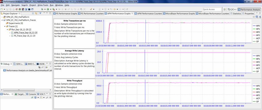
X-Ref Target - Figure 5-4
Figure 5-4: Terminal Settings to View Transcript in SDK
This guide uses various results that are output by the target applications and viewed in the
Terminal 1 panel in SDK. These results include software run-times, achieved bandwidths,
and average latencies.
If you would like to re-create these results and/or run your own, you must connect a USB
cable (Type-A to USB Mini-B) between the UART on the ZC702 board and a USB port on
your host machine.
Figure 5-4 shows the terminal settings required to view this UART transcript in SDK. To view
this pop-up menu, click on the Connect button as shown in the upper-right of Figure 5-3,
page 28. Note that your port may be different than COM5, but all other settings are valid.
System Performance Analysis Send Feedback
29
UG1145 (v2019.1)
(v2018.3)May 22, 2019
December 05, 2018 www.xilinx.comChapter 6
Evaluating Software Performance
There are a number of monitoring capabilities that evaluate software performance on a
Zynq®-7000 SoC. These capabilities can inform you about the efficiency of your application
and provide visualizations for you to better understand and optimize your software.
Performance Monitoring
To illustrate these performance monitoring capabilities, the Bristol/Embecosm Embedded
Energy Benchmark Suite (BEEBS) benchmark program (see Chapter 3, System Performance
Modeling Project) was run on a ZC702 target board and performance results were captured
in the Xilinx® Software Development Kit (SDK) 2015.1. There was no traffic driven from the
Programmable Logic (PL), so this is a software only test. Note that if you would like to
re-create these results, the software application selection is shown in Figure 5-1, page 25,
and the PL traffic is shown in Figure 5-2, page 26. Although the results shown here are for
the BEEBS benchmarks, these exact same metrics can also be obtained for a program
provided to or compiled by SDK.
X-Ref Target - Figure 6-1
Figure 6-1: CPU Utilization Labeled with BEEBS Benchmarks
There are 24 total tests performed – each of the eight benchmarks listed in Table 3-1,
page 16 is run on the three different data array sizes (that is, 4 KB, 64 KB, and 1024 KB).
Because a sleep time of 1 second was inserted between each test, the CPU utilization gives
a clear view of when these benchmarks were run. Figure 6-1 helps orient the timeline for the
results. The three data sizes were run from smallest to largest within each benchmark, which
can be seen in the value and length of the utilization of CPU0. It took approximately 45
seconds to run BEEBs benchmark without any traffic.
System Performance Analysis Send Feedback
30
UG1145 (v2019.1)
(v2018.3)May 22, 2019
December 05, 2018 www.xilinx.comChapter 6: Evaluating Software Performance
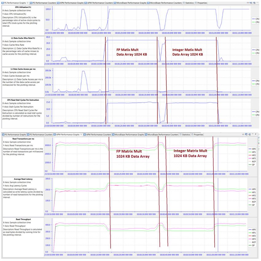
X-Ref Target - Figure 6-2
Figure 6-2: Performance Analysis of BEEBS Benchmarks - CPU Utilization, IPC, L1 Data Cache
Figure 6-2 shows four different graphs displayed by SDK in the PS Performance panel: CPU
Utilization (%), CPU Instructions Per Cycle, L1 Data Cache Access, and L1 Data Cache Miss
Rate (%).
While CPU Utilization helps determine when benchmarks were run, the most insightful
analysis is achieved when multiple graphs are considered. For these particular tests, the
significant analysis comes from the Instructions Per Cycle (IPC) and the L1 data cache
graphs. IPC is a well-known metric to illustrate how software interacts with its environment,
particularly the memory hierarchy. See Computer Organization & Design: The
Hardware/Software Interface by David A. Patterson and John L. Hennessy ([Ref 10]). This
fact becomes evident in Figure 6-2 as the value of IPC follows very closely the L1 data cache
accesses. Also, during the memory-intensive matrix multipliers, the lowest values of IPC
correspond with the highest values of L1 data cache miss rates. If IPC is a measure of
software efficiency, then it is clear from Figure 6-2 that the lowest efficiency is during long
periods of memory-intensive computation. While sometimes this is unavoidable, it is clear
that IPC provides a good metric for this interaction with the memory hierarchy.
System Performance Analysis Send Feedback
31
UG1145 (v2019.1)
(v2018.3)May 22, 2019
December 05, 2018 www.xilinx.comChapter 6: Evaluating Software Performance
X-Ref Target - Figure 6-3
Figure 6-3: Performance Analysis of BEEBS Benchmarks - L1 Data Cache, Stall Cycles Per
Instruction
Taking this analysis one step further, the graphs in Figure 6-3 provide information on data
locality; that is, where the processor retrieves and writes data as it performs the specified
algorithms. A low L1 data cache miss rate means that a significant amount of data is stored
and accessed from that respective cache. A high L1 miss rate coupled with high values in
CPU write or read stall cycles per instruction means that much of the data is coming from
DDR.
As expected, an understanding of the software application aids in the analysis. For example,
the two long periods of high L1 miss rate and CPU read stall cycles shown in Figure 6-3 are
when the floating-point and integer matrix multiplier algorithms are operating on the 512
x 512 (256K words = 1024 KB) two-dimensional or 2-D data array.
To refine the performance of an application, one option to consider using is to
enable/disable the L2 data cache prefetch. This is specified with bit 28 of reg15_prefetch_ctrl
(absolute address 0xF8F02F60). If this data prefetching is enabled, then the adjacent cache
line will also be automatically fetched. While the results shown in Figure 6-2, page 31 and
Figure 6-3 were generated with prefetch enabled, the BEEBS benchmarks were also run with
prefetch disabled. The integer matrix multiplication saw the largest impact on software
run-time with a decrease of 9.0%. While this prefetch option can improve the performance
of some applications, it can lower the performance of others. It is recommended to verify
run-times of your application with and without this prefetch option.
System Performance Analysis Send Feedback
32
UG1145 (v2019.1)
(v2018.3)May 22, 2019
December 05, 2018 www.xilinx.comChapter 6: Evaluating Software Performance
X-Ref Target - Figure 6-4
Figure 6-4: Run-Time Results of Software in BEEBS Benchmark Suite
As mentioned above, a helpful measurement of overall software performance is the
run-time of different portions of the application. Figure 6-4 shows a summary of run-times
for the eight BEEBS benchmarks as run on the three different data array sizes (see
Instrumenting Hardware, page 61 on how these run-times were calculated and captured).
The Y-axis on the left side of Figure 6-4 shows the full range of values, while the Y-axis on
the right side zooms in on the lowest range for clarity. As expected, the run-times increase
with larger array sizes. However, the amount of increase varies across the different
benchmarks tested. This is because there are a number of different factors that can impact
run-time, including the amount of data, data locality, and algorithmic dependencies on data
size. As far as data locality, the 4 KB, 64 KB, and 1024 KB data arrays fit into the L1 data
cache, L2 data cache, and DDR, respectively.
For more information on assessing the performance of the memory hierarchy, see
Chapter 9, Evaluating Memory Hierarchy and the ACP
Visualizing Performance Improvements
As shown in Figure 6-4 the longest run-times are clearly the matrix multiplications,
especially for the largest array size. What if these run-times need to be improved? How
would the performance analysis features in SDK help measure and visualize any code
optimizations or improvements?
The sample code below shows two different C/C++ implementations for floating-point
matrix multiplication. The original and traditional implementation is the Multiply_Old()
function, whereas a newer implementation is contained in Multiply_New(). While the newer
implementation appears to be more complicated, it takes advantage of the 32 byte cache
lines. See What Every Programmer Should Know About Memory by Ulrich Drepper
([Ref 11]).
System Performance Analysis Send Feedback
33
UG1145 (v2019.1)
(v2018.3)May 22, 2019
December 05, 2018 www.xilinx.comChapter 6: Evaluating Software Performance
#define CLS 32
#define SM (CLS / sizeof (float))
/* Original method of calculating floating-point matrix multiplication */
void Multiply_Old(float **A, float **B, float **Res, long dim)
{
for (int i = 0; i < dim; i++) {
for (int j = 0; j < dim; j++) {
for (int Index = 0; Index < dim; Index++) {
Res[i][j] += A[i][Index] * B[Index][j];
}}}
}
/* Modified method of calculating floating-point matrix multiplication */
void Multiply_New(float **A, float **B, float **Res, long dim)
{
for (int i = 0; i < dim; i += SM) {
for (int j = 0; j < dim; j += SM) {
for (int k = 0; k < dim; k += SM) {
float *rres = &Res[i][j];
float *rmul1 = &A[i][k];
for (int i2 = 0; i2 < SM; ++i2, rres += dim, rmul1 += dim) {
float *rmul2 = &B[k][j];
for (int k2 = 0; k2 < SM; ++k2, rmul2 += dim) {
for (int j2 = 0; j2 < SM; ++j2) {
rres[j2] += rmul1[k2] * rmul2[j2];
X-Ref Target - Figure 6-5
Figure 6-5: Original and Modified C/C++ Software for Floating-Point Matrix Multiplication.
The BEEBS benchmark software was re-compiled and re-run using the new implementations
for both floating-point and integer matrix multiplications.
Table 6-1, page 34 lists a summary of the performance metrics reported for CPU0 in the
APU Performance Summary panel in SDK. Even though only 2 of the 8 benchmarks were
modified, there was a noticeable difference in the reported metrics. The average IPC value
increased by 34.9%, while there was a substantial drop in L1 data cache miss rate. The read
stall cycles also decreased dramatically, revealing the reduction in clock cycles when the
CPU is waiting on a data cache refill.
Table 6-1: CPU0 Performance Summary with Original and Modified Matrix Multipliers
CPU0 Performance Summary
Performance Metric
Original Modified Changes
CPU Utilization (%) 100.00 100.00 ≈
CPU Instructions Per Cycle 0.43 0.58 ↑
L1 Data Cache Miss Rate 8.24 0.64 ↓↓
(%)
L1 Data Cache Accesses 3484.33M 3653.48M ≈
System Performance Analysis Send Feedback
34
UG1145 (v2019.1)
(v2018.3)May 22, 2019
December 05, 2018 www.xilinx.comChapter 6: Evaluating Software Performance
Table 6-1: CPU0 Performance Summary with Original and Modified Matrix Multipliers
CPU0 Performance Summary
Performance Metric
Original Modified Changes
CPU Write Stall Cycles Per 0.00 0.00 ≈
Instruction
CPU Read Stall Cycles Per 0.79 0.05 ↓↓
Instruction
X-Ref Target - Figure 6-6
Figure 6-6: Performance Analysis of BEEBS Benchmarks with Improved Matrix Multipliers
Figure 6-6 shows the L1 data cache graphs and CPU stall cycles per instruction reported in
the PS Performance panel. In contrast to Figure 6-3, page 32, it becomes clear that the
bottlenecks of the code – the floating-point and integer matrix multiplications – have been
dramatically improved. The long periods of low IPC, high L1 data cache miss rate, and high
CPU read stall cycles toward the end of the capture have been shortened and improved
considerably.
This is confirmed with software run-times. A summary of the measured run-times is also
listed in Table 6-2. The run-times of the floating-point and integer matrix multiplications
were reduced to 22.8% and 17.0% of their original run-times, respectively.
System Performance Analysis Send Feedback
35
UG1145 (v2019.1)
(v2018.3)May 22, 2019
December 05, 2018 www.xilinx.comChapter 6: Evaluating Software Performance
Table 6-2: Summary of Software Run-Times for Original and Modified Matrix Multipliers
Software Run-Times (msec)
Benchmark
Original Modified
9201.70 2100.36
Floating-point matrix multiplication
100.0% 22.8%
8726.67 1483.24
Integer matrix multiplication
100.0% 17.0%
System Performance Analysis Send Feedback
36
UG1145 (v2019.1)
(v2018.3)May 22, 2019
December 05, 2018 www.xilinx.comChapter 7
Evaluating High-Performance Ports
A great benefit provided by System Performance Modeling (SPM) is to perform what if
scenarios of Processing System (PS) and Programmable Logic (PL) activity and their
interaction. This is a feature that enables you to explore performance before beginning the
design phase, thus reducing the likelihood of finding performance issues late in the design.
Although contention on the Zynq®-7000 SoC device is not directly visualized, its impact on
system performance is displayed.
You can configure the SPM design to model specific traffic scenarios while running a
software application in the PS. You can then use PL master performance metrics, such as
throughput and latency, to verify that the desired system performance can be sustained in
such an environment. This process can be repeated multiple times using different traffic
scenarios.
One critical shared resource on the Zynq-7000 SoC device is the DDR controller. This
resource is shared by both CPUs, the four High-Performance (HP) ports, the Accelerator
Coherency Port (ACP), and other masters via the central interconnect (see Chapter 8,
Evaluating DDR Controller Settings for more details). Because of this sharing, it is important
to understand the available DDR bandwidth.
You can calculate the total theoretical bandwidth of the DDR using the following equation:
(533.3 Mcycles)/sec x (2 tranx)/cycle× (4 bytes)/tranx=4270 MB/sec Equation 1
While this is the maximum bandwidth achievable by this memory, the actual DDR utilization
is based on many factors, including number of requesting masters and the types of memory
accesses. As shown in this chapter, requesting bandwidth that approaches or exceeds this
maximum will potentially impact the achieved throughput and latency of all requesting
masters. The System Performance Analysis (SPA) toolbox in the Xilinx® Software
Development Kit (SDK) aids in this analysis.
HD Video Traffic
The software application used was the Bristol/Embecosm Embedded Energy Benchmark
Suite (BEEBS) benchmark program described in SPM Software, page 15. See Figure 5-1,
page 25, which shows how this can be specified in SDK. In this scenario, traffic on the four
High Performance (HP) ports was injected into the system, and software and hardware
performance metrics are measured in SDK. This models a system that is performing
System Performance Analysis Send Feedback
37
UG1145 (v2019.1)
(v2018.3)May 22, 2019
December 05, 2018 www.xilinx.comChapter 7: Evaluating High-Performance Ports
complex algorithms in software while simultaneously processing HD video streams in the
PL. Rather than design a system that implements this processing, you can instead model the
performance using SPM. You can quickly verify that your desired performance is achieved
even before beginning your design.
X-Ref Target - Figure 7-1
Figure 7-1: ATG Traffic Configuration Modeling HD Video Streams on HP Ports
Figure 7-1 shows the first traffic scenario used (see Chapter 5, Getting Started with SPM for
a description of this traffic specification). This scenario models four uncompressed
1080p/60 (that is, 1080 lines, progressive, and 60 frames/sec) HD video streams. Two
streams are being read from the DDR on ports HP0 and HP2, while two are being written on
ports HP1 and HP3. For all of these modeled video streams, the Tranx Interval was chosen
to request 376 MB/sec, the estimated throughput of the uncompressed RGB 4:4:4 video.
System Performance Analysis Send Feedback
38
UG1145 (v2019.1)
(v2018.3)May 22, 2019
December 05, 2018 www.xilinx.comYou can also read