A lead-width distribution for Antarctic sea ice: a case study for the Weddell Sea with high-resolution Sentinel-2 images - The Cryosphere
←
→
Page content transcription
If your browser does not render page correctly, please read the page content below
The Cryosphere, 15, 4527–4537, 2021
https://doi.org/10.5194/tc-15-4527-2021
© Author(s) 2021. This work is distributed under
the Creative Commons Attribution 4.0 License.

A lead-width distribution for Antarctic sea ice: a case study for the
Weddell Sea with high-resolution Sentinel-2 images
Marek Muchow1 , Amelie U. Schmitt2 , and Lars Kaleschke3
1 Institute
          of Oceanography, Center for Earth System Research and Sustainability (CEN),
Universität Hamburg, Hamburg, Germany
2 Meteorological Institute, Center for Earth System Research and Sustainability (CEN),

Universität Hamburg, Hamburg, Germany
3 Alfred-Wegener-Institut, Helmholtz-Zentrum für Polar- und Meeresforschung, Bremerhaven, Germany

Correspondence: Marek Muchow (marek.muchow@uni-hamburg.de)

Received: 5 August 2020 – Discussion started: 18 August 2020
Revised: 22 June 2021 – Accepted: 17 August 2021 – Published: 28 September 2021

Abstract. Using Copernicus Sentinel-2 images we derive a           1   Introduction
statistical lead-width distribution for the Weddell Sea. While
previous work focused on the Arctic, this is the first lead-
width distribution for Antarctic sea ice. Previous studies sug-    Leads are created by dynamic motions of the sea ice (Miles
gest that the lead-width distribution follows a power law with     and Barry, 1998) and covered by open water or thin sea ice.
a positive exponent; however their results for the power-law       They often follow a linear-like shape, can be up to tens of
exponents are not all in agreement with each other.                kilometers long and are by definition a few meters to some
   To detect leads we create a sea-ice surface-type classifi-      kilometers wide (e.g., Alam and Curry, 1997). An adequate
cation based on 20 carefully selected cloud-free Sentinel-2        representation of leads in climate models is important for var-
Level-1C products, which have a resolution of 10 m. The ob-        ious processes. Leads play a large role in the absorption of
served time period is from November 2016 until February            shortwave radiation due to the low albedo of open water and
2018, covering only the months from November to April.             nilas, compared to the higher albedo of thicker ice and snow-
We apply two different fitting methods to the measured lead        covered sea ice (Perovich, 1996). Newly formed leads are
widths. The first fitting method is a linear fit, while the sec-   also an important area for ice production and the associated
ond method is based on a maximum likelihood approach.              brine rejection to the ocean below (Alam and Curry, 1997).
Here, we use both methods for the same lead-width data set            Furthermore, the heat exchange between atmosphere and
to observe differences in the calculated power-law exponent.       ocean is strongly enhanced over leads. Using a simple heat
   To further investigate influences on the power-law expo-        flux model, Maykut (1978) found that the heat loss over thin
nent, we define two different thresholds: one for open-water-      ice (0.4–0.5 m) is 1 order of magnitude larger than over mul-
covered leads and one for open-water-covered and nilas-            tiyear ice. In a model study, Lüpkes et al. (2008) demon-
covered leads. The influence of the lead threshold on the          strated that an increase in the lead fraction area by 1 % dur-
exponent is larger for the linear fit than for the method          ing the polar night can lead to local air temperature warming
based on the maximum likelihood approach. We show that             of up to 3.5 K. Based on buoy data in the Weddell Sea re-
the exponent of the lead-width distribution ranges between         gion combined with a thermodynamic sea-ice model, Eisen
1.110 and 1.413 depending on the applied fitting method and        and Kottmeier (2000) found that leads contribute roughly
lead threshold. This exponent for the Weddell Sea sea ice is       30 % to the total energy flux from the ocean to the atmo-
smaller than the previously observed exponents for the Arctic      sphere in winter months. Due to the large temperature dif-
sea ice.                                                           ferences between the air and the lead surface in winter, con-
                                                                   vective plumes forming over leads can have a large impact
                                                                   on the atmospheric processes in regions covered with sea ice

Published by Copernicus Publications on behalf of the European Geosciences Union.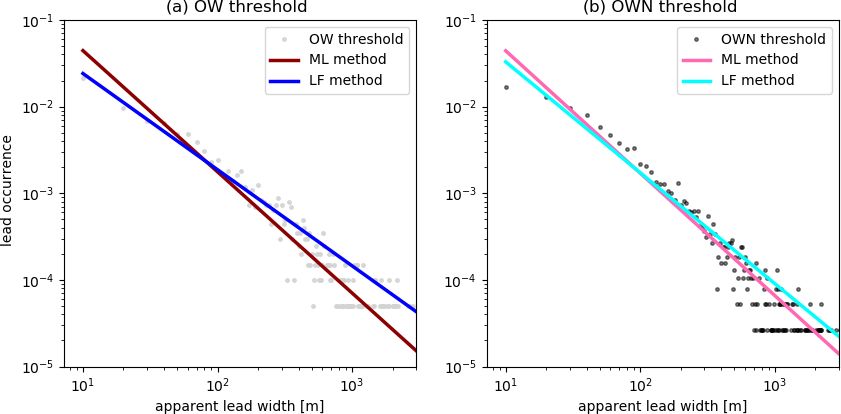
4528                                                         M. Muchow et al.: A lead-width distribution for Antarctic sea ice

(e.g., Tetzlaff et al., 2015; Lüpkes et al., 2008; Chechin et al.,   sea ice, the TOA reflectance is related to the ice thickness.
2019).                                                               As a first step, we introduce a surface-type classification
   Different studies suggested that the overall heat exchange        for the Sentinel-2 satellite products to identify different sea-
over leads depends not only on lead area fraction or ice thick-      ice types and leads (Sect. 3.1). The determined reflectance
ness but also on lead width. Using a fetch-dependent formu-          thresholds for leads covered with open water and nilas are
lation of the heat exchange, Marcq and Weiss (2012) demon-           then used to detect leads and calculate a lead-width distri-
strated that the heat transfer is 2 times more effective for nar-    bution. Since some of the previous studies focused on leads
row leads of several meters than for wider ones of several           covered only by open water and others also included leads
hundreds of meters. Furthermore, Qu et al. (2019) used a             covered by thin sea ice, we apply two different reflectance
combination of remote sensing and reanalysis data and found          thresholds and compare the results. Subsequently, a power
that narrow leads (≤ 1 km) accounted for about a quarter of          law is fitted to the resulting lead-width distribution. We apply
the heat flux over all leads.                                        two different statistical methods to determine the power-law
   To account for these lead-width-dependent processes in            exponents, which have both been used in different previous
models, the lead width needs to be parametrized. One pos-            studies, and compare the results (Sect. 3.2). The results are
sibility is to apply a lead-width distribution. Several studies      presented and discussed in Sect. 4, followed by conclusions
estimating shear and divergence rates for Arctic sea ice us-         in Sect. 5.
ing satellite observations suggest that these quantities follow
a power law (e.g., Marsan et al., 2004; Stern and Lindsay,
2009). Such a power-law scaling has also been found in dif-          2   Data
ferent modeling studies (e.g., Girard et al., 2009; Wang et al.,
                                                                     The two sun-synchronous Sentinel-2 satellites carry the pas-
2016; Ólason et al., 2021). Since leads are formed by diver-
                                                                     sively working MultiSpectral Instrument (MSI) with 13 dif-
gent sea-ice motions, it is plausible to also expect a power-
                                                                     ferent spectral bands from 443 nm (visible) to 2190 nm
law behavior for lead width. Power-law exponents for lead
                                                                     (shortwave infrared) (ESA, 2018). The spatial resolution for
widths in the Arctic have been derived from submarine mea-
                                                                     the bands is 10, 20 or 60 m while the images cover an area of
surements (Wadhams, 1981; Wadhams et al., 1985), as well
                                                                     100 × 100 km. A higher resolution allows for the detection
as from remote sensing data from thermal imagers (Lindsay
                                                                     of narrower leads. We therefore visually compared all 10 m
and Rothrock, 1995; Qu et al., 2019), visible imagery (Marcq
                                                                     bands (2, 3, 4 and 8) to identify the band with the best repre-
and Weiss, 2012) and altimetry (Wernecke and Kaleschke,
                                                                     sentation of thin ice structures. The best results were found
2015). Since data with different resolutions were used in
                                                                     for band 4 (665 nm), which is then used for the analysis in
these studies, there are substantial differences in the methods
                                                                     this study.
used to detect leads and in the minimum lead widths con-
                                                                        We selected the Weddell Sea as a case study, since
sidered. In addition, different statistical methods have been
                                                                     Sentinel-2 is a land mission and acquires data over oceans
applied to calculate the power-law exponents. Consequently,
                                                                     only in the vicinity of land (Drusch et al., 2012), which re-
obtained values for the power-law exponent from observa-
                                                                     stricts the regional selection. Due to the need for sunlight
tions vary in absolute values and the suitable range of the
                                                                     to capture suitable data, only Sentinel-2 Level-1C products
distribution.
                                                                     covering the months from November to April were used.
   For the Antarctic, different studies have derived lead frac-
                                                                     The Weddell Sea contains a large enough sea-ice cover dur-
tions (Allison et al., 1993; Reiser et al., 2020; Petty et al.,
                                                                     ing these months (e.g., Comiso and Nishio, 2008). Addition-
2021); however lead-width distributions have not been stud-
                                                                     ally, only products classified as cloud-free were selected in
ied, yet. In this study, we derive a lead-width distribution for
                                                                     the Copernicus Open Access Hub (https://scihub.copernicus.
the Weddell Sea sea ice as a case study for Antarctic sea ice.
                                                                     eu/dhus/#/home, last access: 22 August 2020). We noticed
For this purpose, we introduce a new method to derive lead
                                                                     that in products with wide leads small clouds often occur,
widths using Sentinel-2 data. The main goals of this study
                                                                     most likely from moisture and heat flux through the lead.
are (1) to demonstrate that Sentinel-2 data are suitable for
                                                                     Those images were rejected manually, and we only use to-
deriving lead widths and (2) to determine whether a power-
                                                                     tally cloud-free images. Thus, the final 20 Sentinel-2 Level-
law behavior – with an exponent similar to previous results
                                                                     1C products are always between the months of November
for the Arctic – can also be found for Antarctic sea ice in the
                                                                     to April, while the whole observation period ranges from
Weddell Sea.
                                                                     November 2016 until February 2018 (Fig. 1).
   The main advantage of the recently launched Sentinel-2
                                                                        The lead-width detection method (Sect. 3.2) is applied
satellites is their high resolution up to 10 m. This enables
                                                                     to all 20 products. The classification of surface types and
us to also detect very narrow leads, which most of the for-
                                                                     threshold identification (Sect. 3.1) is based on 9 of those 20
mer studies were not capable of. We use cloud-free Sentinel-
                                                                     products from January to April 2017. For more details on the
2 Level-1C products, which give the top-of-the-atmosphere
                                                                     data see Table 1.
(TOA) reflectance (Drusch et al., 2012). The data are de-
scribed in Sect. 2. Similarly to the albedo for young, thin

The Cryosphere, 15, 4527–4537, 2021                                                     https://doi.org/10.5194/tc-15-4527-2021
M. Muchow et al.: A lead-width distribution for Antarctic sea ice 4529
Figure 1. Display of the selection steps for the 20 Sentinel-2 Level-1C products. The location of the 20 different Sentinel-2 Level-1C
products for this study is the Weddell Sea. Of the 20 products, 9 were used for the sea-ice surface-type classification (red border), while for
the lead-width detection all 20 were used (red and blue border). For the border of the product the “real image outlines” are displayed, which
are not always rectangular since the satellite swath does not always overlap completely with the processing grid applied by ESA. Displayed
in gray is the Antarctic continent border including the shelf ice border measured with different satellite radar from 2007–2009 (Mouginot
et al., 2017; Rignot et al., 2013).
Table 1. Sentinel-2 Level-1C products used for measuring the lead width. Products which are also used for the classification are labeled with
“yes”.
Sensing date (dd/mm/yyyy) Classification Product name
12/11/2016 no S2A_MSIL1C_20161112T104212_N0204_R122_T26CMC_20161112T104210
20/11/2016 no S2A_MSIL1C_20161120T100152_N0204_R093_T25CES_20161120T100153
20/11/2016 no S2A_MSIL1C_20161120T100152_N0204_R093_T25CDS_20161120T100153
29/11/2016 no S2A_MSIL1C_20161129T103152_N0204_R079_T24CXE_20161129T103151
20/12/2016 no S2A_MSIL1C_20161220T100052_N0204_R093_T24CVV_20161220T100049
23/02/2017 yes S2A_MSIL1C_20170223T123141_N0204_R023_T21CVT_20170223T123144
23/02/2017 no S2A_MSIL1C_20170223T123141_N0204_R023_T22DDF_20170223T123144
23/02/2017 no S2A_MSIL1C_20170223T123141_N0204_R023_T22DDG_20170223T123144
24/02/2017 yes S2A_MSIL1C_20170224T120231_N0204_R037_T22CEC_20170224T120234
26/02/2017 yes S2A_MSIL1C_20170226T110241_N0204_R065_T23CNQ_20170226T110244
02/03/2017 no S2A_MSIL1C_20170302T122211_N0204_R123_T22CDD_20170302T122205
13/03/2017 no S2A_MSIL1C_20170313T101141_N0204_R136_T25CDS_20170313T101144
16/03/2017 yes S2A_MSIL1C_20170316T102141_N0204_R036_T25CES_20170316T102141
16/03/2017 yes S2A_MSIL1C_20170316T102141_N0204_R036_T25CES_20170316T102141
16/03/2017 yes S2A_MSIL1C_20170316T102141_N0204_R036_T24CWC_20170316T102141
06/04/2017 yes S2A_MSIL1C_20170406T131051_N0204_R052_T21DVF_20170406T131050
06/04/2017 yes S2A_MSIL1C_20170406T131051_N0204_R052_T21DVG_20170406T131050
06/04/2017 yes S2A_MSIL1C_20170406T131051_N0204_R052_T21DVD_20170406T131050
06/04/2017 no S2A_MSIL1C_20170406T131051_N0204_R052_T20DPJ_20170406T131050
09/02/2018 no S2A_MSIL1C_20180209T120241_N0206_R037_T21CWU_20180209T163245
3 Methods face type is created and the Gaussian curves are fitted to each
data set. Third, the results from the surface classification are
3.1 Threshold identification used to identify two thresholds, which are later used for cre-
ating binary “lead–sea-ice” images for the lead-width mea-
The threshold identification contains the following main surement.
steps (Fig. 2): first, five different surface types are classi- For the surface-type classification 9 out of 20 later-used
fied based on the top-of-the-atmosphere (TOA) reflectance. Sentinel-2 Level-1C products are utilized (Sect. 2). We iden-
Second, a TOA reflectance probability data set for each sur-
https://doi.org/10.5194/tc-15-4527-2021 The Cryosphere, 15, 4527–4537, 20214530 M. Muchow et al.: A lead-width distribution for Antarctic sea ice
Figure 2. Data analysis steps for obtaining the Gaussian curves for each surface type.
tify five different surface types including open water and heat exchange to open-water leads. Additionally, leads are
four different ice types (nilas, gray sea ice, gray-white sea defined as being navigable by surface vessels (WMO, 2014),
ice and sea ice covered with snow). The names of the sea- which is still true for leads covered with nilas.
ice categories are based on the WMO Sea-Ice Nomenclature
(WMO, 2014) for consistency with other literature. However, 3.2 Measuring the apparent lead width and
we want to stress that our classification is based on the TOA determining the power-law exponent
reflectance and not on sea-ice age or thickness. On every
band-4 image, 10 areas of each surface type are masked man- Since the leads within each image can have arbitrary orien-
ually. Thereafter, the TOA reflectance of each pixel within tations, it is not guaranteed that the “true lead width” orthog-
the mask is used to create a reflectance value data set for each onally to the leads’ orientation is measured but the width of
surface type. The reflectance values lie between zero and 1. a line across the lead at an angle other then 90◦ . As in Wer-
To analyze the range of the TOA reflectance for each sur- necke and Kaleschke (2015) we call the measured lead width
face type, histograms are created, which show the occurrence the apparent lead width as a proxy for the true lead width. To
of pixels with a specific TOA reflectance. These histograms measure the apparent lead width we use a measurement grid
are used to fit a summation over Gaussian functions with the consisting of 10 vertical and 10 horizontal equally spaced
mean µ and standard deviation σ to the data: measurement tracks across each Sentinel-2 product (Fig. 4).
n
x−µi
2 The obtained data set of apparent lead widths can then
X 1 −0.5 σi be displayed as a histogram showing the occurrence p(x)
y(x) = ai · √ ·e . (1)
i=1 2π σi for each specific width. As has been carried out in previ-
ous studies (Wadhams, 1981; Wadhams et al., 1985; Lindsay
n indicates the number of Gaussian curves that were com- and Rothrock, 1995; Marcq and Weiss, 2012; Wernecke and
bined into one function and weighted with the weighting pa- Kaleschke, 2015; Qu et al., 2019), we assume that the shape
rameter ai , for fitting the histograms. By using n > 1 we can of the histogram follows a power law with the exponent α
account for multiple maxima in a distribution. Thus, n = 2 is and the apparent lead widths xwidth :
used for gray-white sea ice and n = 3 for gray sea ice (Fig. 3).
One Gaussian curve (n = 1) is fitted to the histogram for open −α
water, nilas and sea ice covered with snow. p(x) = C · xwidth . (2)
The threshold for each surface category is then determined
as the values of the TOA reflectance at the point of intersec- The scaling parameter C is the offset at the y axis and there-
tion of two curves adjacent to each other. An exception is the fore related to the number of measurements, and it is not fur-
threshold for open water, where two points of intersection ther investigated here.
occur. In this case the second point of intersection is chosen We apply two different methods to estimate the power-law
to be the threshold because the first point of intersection is exponent α. For the linear fit (LF method) the apparent lead
before the maximum. The area of intersection of two curves widths are sorted by size so that the frequency p(x) of the
is then the overlap error of those thresholds and describes specific width is available. On a plot with both logarithmic
where we manually classified pixels with the same TOA re- axes, the distribution of the data follows a straight line with
flectance in different sea-ice surface categories. a specific slope and an axis intercept. The slope is the rep-
For the lead identification two different thresholds are used resentation of the power-law exponent α. Due to the same
to create binary images: one for leads covered with open wa- influence of every value for the result of the fit, atypical val-
ter (OW threshold) and one for leads covered with open water ues have a strong effect on the result (Berk, 2004).
and nilas (OWN threshold). We decided to use two thresholds The second method for estimating the exponent α is the
to observe the effect of the coverage of the lead on the power method for discrete values by Clauset et al. (2009), which is
law similarly to Marcq and Weiss (2012), who used two dif- based on a maximum likelihood approach (ML method). The
ferent luminance thresholds for leads. Additionally, we de- power-law distribution diverges at zero; therefore a lower
cided to use the combined OWN threshold since open water boundary xmin > 0 is needed. In this study, xmin is the small-
refreezes quickly in leads depending on the surrounding tem- est possible apparent lead width, which is the image resolu-
peratures, but the leads keep similar properties in regards to tion of 10 m. The following equation is used for estimating
The Cryosphere, 15, 4527–4537, 2021 https://doi.org/10.5194/tc-15-4527-2021M. Muchow et al.: A lead-width distribution for Antarctic sea ice 4531
Figure 3. The number of pixels within every surface type for a specific TOA reflectance. The TOA reflectance threshold for each surface
type is the point of intersection of two curves adjacent to each other. The error is shown as the overlap error of these two curves below each
threshold. The red arrows show the two thresholds later used for the lead identification for the lead-width measurement: the open-water (OW)
threshold and the open-water-and-nilas (OWN) threshold.
Figure 4. (a) Exemplary original Sentinel-2 Level-1C band-4 image (sensing date: 16 March 2017). (b) Binary image after the application
of the open-water-and-nilas (OWN) threshold, where leads are indicated with black pixels and no leads with white ones. (c) Applied mea-
surement grid with 10 horizontal and vertical measurement tracks. The swath of the Sentinel-2 satellite does not cover the whole image area
defined by the ESA data-processing grid. Thus, only the area covered by the satellite swath is considered for the lead-width measurement.
the power-law exponent α: olution of 10 m, the “step size” in Eq. (3) is set to 10 m simi-
" !#−1 larly to in Wernecke and Kaleschke (2015).
n To reduce the influence of possible single outlying mea-
X xwidth,i
αu1 + n · ln . (3) surements on the result of the power-law exponent, we esti-
i=1 xmin − 21 · step size
mated the lead-width distribution 100 times with a random
The total number of counted leads is n, and xwidth,i is the selection of 70 % of the measured apparent lead widths. We
measured lead widths. Since the data are discrete with a res- choose 70 % to still have enough measured widths while hav-
https://doi.org/10.5194/tc-15-4527-2021 The Cryosphere, 15, 4527–4537, 20214532 M. Muchow et al.: A lead-width distribution for Antarctic sea ice
Table 2. The table displays the threshold for each surface type from nificant difference. To evaluate the two thresholds, which are
the surface classification. The thresholds are the point of intersec- later used for the lead detection, they are compared to mea-
tion between the Gaussian curves describing the TOA reflectance sured albedo values from the East Antarctic sea-ice zone in
values that occurred for each surface type (Fig. 3, Sect. 3.1). Every austral spring and summer by Brandt et al. (2005). Their es-
threshold contains the surface types that are above it in the table. timated albedos for open water (0.07) and nilas without snow
Sea ice covered with snow has no estimated threshold; therefore it
cover (0.14) are close to the thresholds estimated here for the
is indicated as 1.0.
same surface types. For the classification of the two later-
Surface type Threshold (TOA Overlap used thresholds we aimed to classify structures without snow
reflectance) error (%) cover. For the other surface types it is much more difficult
to make assumptions about the snow cover or thickness due
Open water 0.10 to the fact that only the reflectance values are known. Nev-
29
ertheless, our estimated TOA reflectance thresholds for each
Nilas 0.17 surface type are always in the range of the reference albedo
11 measurements from Brandt et al. (2005).
Gray sea ice 0.44 Additionally, since leads normally have sharp edges the
3 selection of areas as example values for open water and nilas
was comparatively easy compared to the other sea-ice surface
Gray-white sea ice 0.66 types. The thicker the ice and snow cover, the more unreliable
4
these observations become. To obtain a more precise classifi-
Sea ice covered with snow 1.0 cation of the surface types’ validation with other data sources
like field measurements could be beneficial. Nevertheless,
the TOA reflectance thresholds (0.10 for OW and 0.16 for
ing variation between the data sets. The final power-law ex- OWN) were used for the lead detection and agree with val-
ponent is then estimated as the mean over the 100 calcula- ues from previous measurements (Brandt et al., 2005).
tions. Additionally, as a measure for uncertainty, the standard
deviation is also estimated from the 100 calculations. 4.2 Measured lead widths and the power-law exponent
The lead-width distribution derived from 20 Sentinel-2 prod-
4 Results and discussion ucts using both the open-water (OW) and the open-water-
and-nilas (OWN) threshold is presented in Fig. 5. The total
4.1 Threshold identification number of leads observed with the OW threshold is 2024,
while for the OWN threshold 3799 leads are observed. The
The thresholds between surface categories and correspond- largest observed apparent lead widths are 6500 m for the OW
ing overlap errors are determined using the method described threshold and 6530 m for the OWN threshold. Looking at the
in Sect. 3.1. With Sentinel-2 band-4 images it is possible to distribution of the measured lead widths, it is evident that the
distinguish between five different surface types (open water, small leads dominate and that with an increasing width the
nilas, gray sea ice, gray-white sea ice, sea ice covered with number of leads decreases. We measured leads with a width
snow) based on top-of-the-atmosphere (TOA) reflectance from 10 m down to the resolution of the Sentinel-2 band-4
values (Fig. 3). The results for the thresholds and the cor- image resolution and upwards, but the number of measured
responding overlap error are presented in Table 2. Note that leads with a width of 10 m is lower than what might be ex-
for the lead identification only two thresholds are applied: the pected (Figs. 5 and 6). One possible reason is the resolution
open-water (OW) threshold and a threshold combining open itself, and according to Wernecke and Kaleschke (2015) this
water and nilas (OWN). is a typical feature with fewer measurements for the lower
The common value used to compare optical properties of bound of the resolution, since a 10 m lead is not always cov-
sea ice is the albedo. In this study, we measure TOA re- ered completely by 1 image pixel but partially by 2 or more,
flectance instead of albedo. Both properties increase with the so the signal of the lead is not detected. The upper limit of the
sea ice and snow cover thickness, especially for young, thin power-law range is cut off by the availability of wider leads,
sea ice in the absence of melting processes. In addition to since wider leads tend to produce small clouds and we only
this, we only use cloud-free Sentinel-2 band-4 images. Thus, analyzed cloud-free data.
the atmosphere has a negligible influence on the reflectance As described in Sect. 3.2 we apply two different methods
measurement. We estimated the thresholds with Sentinel-2 to fit a power law to the lead-width distribution. The cal-
band-4 images from January to April 2017 to include differ- culated power-law exponents for both thresholds and fitting
ent sun and look angles. Before estimating the thresholds we methods are presented at the bottom of Table 3. At first we
also compared the TOA reflectance values for each surface compare the results for the same thresholds with different
type within the products with each other and found no sig- methods to one another (Fig. 5) to estimate the impact of
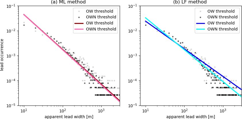
The Cryosphere, 15, 4527–4537, 2021 https://doi.org/10.5194/tc-15-4527-2021M. Muchow et al.: A lead-width distribution for Antarctic sea ice 4533 Figure 5. Relative lead occurrence as a function of measured lead width (dots). Lead widths were measured using (a) the open-water (OW) threshold and (b) the open-water-and-nilas (OWN) threshold. Straight lines indicate the fitted power-law curves using the ML and LF method. Figure 6. Same as Fig. 5 but with the results for both thresholds for (a) the ML fitting method and (b) the LF fitting method. the methods. The values for the power-law exponent with nilas. For the LF method the different thresholds give two the OW threshold are 1.110 (LF method) and 1.399 (ML different results of the exponent for the lead-width distribu- method). For this threshold, the method has a strong impact tion power law (OW, 1.110; OWN, 1.280). Otherwise, for the on the result. For the OWN threshold the results are closer ML method the choice of the threshold has no strong influ- (LF method, 1.280; ML method, 1.413). The standard devia- ence on the result of the power-law exponent (OW, 1.399; tion for the LF method is 10 times higher (0.02) than for the OWN, 1.413). Thus, choosing different thresholds or criteria ML method (0.002). These results confirm that the method for the definition of the lead can influence the result. This is has a non-neglectable effect on the result of the exponent for supported by the result of Marcq and Weiss (2012), who used the sea-ice width distribution power law. two differing thresholds which have a similar range to one Secondly, we compare the results for the same method another, as with our estimates for the LF method (Table 3). with both thresholds to show the importance of the choice Previous studies about lead-width distributions (Table 3) of thresholds (Fig. 6). The OW threshold covers only leads focused on different regions in the Arctic and not on Antarc- without any thin sea ice, while the OWN threshold includes tic regions. While observing leads in the Arctic sea ice is open water but also leads covered with sea ice. Thus, the outside the scope of this study, we compare our results with OWN threshold data set includes more lead-width measure- the results from the Arctic sea ice to gain more insight about ments but also wider leads due to lead edges covered with possible effects on the differences. The exponent of the lead- https://doi.org/10.5194/tc-15-4527-2021 The Cryosphere, 15, 4527–4537, 2021
4534                                                            M. Muchow et al.: A lead-width distribution for Antarctic sea ice

Table 3. Different results from the literature and this study for the Weddell Sea sorted by publishing date. The threshold definition for lead
identification differs between the studies. Marcq and Weiss (2012) use two different luminance thresholds. The last two entries are the results
of this study for the Weddell Sea for which two thresholds (OW, open-water-covered leads; OWN, open-water-covered and nilas-covered
leads) are also applied. The LF method stands for a linear fit, and the ML method stays for the method after Clauset et al. (2009). A detailed
explanation of the methods is in Sect. 3.2.

   Source                       Fitting    Platform/      Time and region          Resolution of     Range of the     Power-law exponent
                                method     instrument                              the power law     power law        α
   Wadhams (1981)               LF         submarine      October 1976, Euro-      about 5 m         50–1000 m        2.00
                                           mission        pean Arctic Ocean
   Wadhams et al. (1985)        LF         submarine      February 1967,           about 5 m         50–1000 m        2.29
                                           mission        Davis Strait
   Lindsay and Rothrock         LF         AVHRR          1989, central Arctic     1 km              1–50 km          1.60 ± 0.18
   (1995)                                                 Ocean
   Marcq and Weiss (2012)       ML         SPOT           April 1996, central      10 m              0.02–2 km        2.1–2.3
                                                          Arctic Ocean                                                2.5–2.6
   Wernecke and Kaleschke       ML         CryoSat-2      winter 2011–2014,        300 m             ≥ 600 m          2.47 ± 0.04
   (2015)                                                 Arctic Ocean
   Qu et al. (2019)             LF         MODIS,         April 2015, Beaufort     30 m–1 km         ≥ 30 m           2.241–2.346
                                           Landsat 8      Sea
   This study                   LF         Sentinel-2     2016–2018                10 m              0.01–6.5 km      OW: 1.110 ± 0.020
                                                          (November–April),                                           OWN: 1.280 ± 0.020
                                                          Weddell Sea
   This study                   ML         Sentinel-2     2016–2018                10 m              0.01–6.5 km      OW: 1.399 ± 0.002
                                                          (November–April),                                           OWN: 1.413 ± 0.002
                                                          Weddell Sea

width distribution power law determined by this study for the              quency distributions in the pan-Arctic indicate an influence
Weddell Sea sea ice is smaller than in all previous studies for            of bathymetry and ocean currents. However, the result for the
Arctic sea ice: the results by Wernecke and Kaleschke (2015)               lead-width distribution by Lindsay and Rothrock (1995) also
using the CryoSat-2 satellite support the earlier-mentioned                disagrees with the result from Marcq and Weiss (2012), both
results by Marcq and Weiss (2012) (SPOT satellite) with a                  of which were obtained in the central Arctic Ocean, while
power-law exponent of around 2.50. The power-law expo-                     other previous results are similar (Marcq and Weiss, 2012;
nent found by Qu et al. (2019) (2.241–2.346) using a com-                  Wernecke and Kaleschke, 2015; Qu et al., 2019).
bination of MODIS and Landsat 8 is in the same range as                       Furthermore, the results for the power-law exponent dis-
the first and lower exponent from Marcq and Weiss (2012),                  played in Table 3 are based on a scale-invariant approach;
who also used two thresholds. Furthermore, there were two                  however Qu et al. (2019) used different resolutions of the
surveys using submarines from which power-law exponents                    measured lead width ranging from 30 m to 1 km resulting in
of 2.00 and 2.29 were calculated (Wadhams, 1981; Wad-                      differences in the power-law exponent in the first decimal
hams et al., 1985). The only result below 2.0 is from Lind-                place, indicating that the power-law scaling for lead width
say and Rothrock (1995) with a power-law exponent of 1.60.                 might not always be scale invariant. In addition to that, Ram-
They used data from the Advanced Very High Resolution Ra-                  pal et al. (2019) confirmed a multi-fractal dependence of
diometer (AVHRR).                                                          the sea-ice deformation rates on timescales and space scales.
   In addition to the different measurement systems (differ-               Thus, applying these results to different processes related to
ent satellites and submarines) and different methods regard-               deformation, like leads formed due to divergence, would be
ing lead definition and measurement, the studies for the Arc-              a necessary step for further research.
tic observe leads in different regions (Table 3). Willmes and                 Another possible reason for the differences is the differ-
Heinemann (2016) showed that the sea-ice wintertime lead                   ent conditions in both regions. While the Arctic Ocean is
frequencies differ throughout the Arctic Ocean and identi-                 surrounded by land mass, the Southern Ocean surrounds
fied the marginal ice zone in the Fram Strait and the Bar-                 the Antarctic continent. The Antarctic sea ice is exposed
ents Sea as the primary region for lead activities. Lead fre-              to the Antarctic Circumpolar Current and strong circumpo-

The Cryosphere, 15, 4527–4537, 2021                                                            https://doi.org/10.5194/tc-15-4527-2021
M. Muchow et al.: A lead-width distribution for Antarctic sea ice 4535
lar winds. The Antarctic sea-ice cover is generally more di- and account for possible regional differences in lead widths
vergent than much of the Arctic ice cover (Gloersen et al., throughout the Antarctic sea ice. For future comparison the
1993). Lead fractions in the central Arctic shown by Petty same fitting method should be applied, since our study shows
et al. (2021) are lower compared to in the Southern Ocean, that with the same data different results occur.
which also shows some regional differences. Additionally,
Worby et al. (2008) estimated the long-term mean (1981–
2005) of total Antarctic sea-ice thickness in winter as 0.66 ± Data availability. All Sentinel-2 Level-1C products used are given
0.60 m. For the Arctic Ocean, Kwok et al. (2009) calculated in Table 1. We accessed the data using the Copernicus Open Access
a 5-year mean (2003–2008) ice thickness during winter of Hub (2018, https://scihub.copernicus.eu/dhus/#/home).
2.9 ± 0.3 m. Different sea-ice thicknesses influence the sea
ice to have different rheologic properties (Feltham, 2008).
Author contributions. MM acquired and checked the data, created
the surface-type classification, and derived the lead-width distribu-
tion under the supervision of LK. AUS helped with the derivation
5 Conclusions of the lead-width distribution and editing the paper. MM prepared
the paper with contributions of all co-authors.
We introduce a lead-width distribution for Antarctic sea ice
using the Weddell Sea as a case study. To observe leads and
their width with Sentinel-2 Level-1C products, it is neces- Competing interests. The authors declare that they have no conflict
sary to have a surface-type classification. Therefore we an- of interest.
alyzed Sentinel-2 Level-1C products (band 4, 665 nm) with
a resolution of 10 m and created a surface-type classification
based on the top-of-the-atmosphere (TOA) reflectance. With Disclaimer. Publisher’s note: Copernicus Publications remains
this classification the Sentinel-2 Level-1C data can be used to neutral with regard to jurisdictional claims in published maps and
detect and observe sea-ice leads under cloud-free conditions institutional affiliations.
with a resolution of 10 m. The local overpass time of the two
Sentinel-2 satellites matches the SPOT satellite and is close
to Landsat 8, which provides the possibility for a future com- Acknowledgements. This work was financially supported by the
bination of the data sets to form longer time series. The mis- German Science Foundation (DFG) with the project number
sion lifetime for Sentinel-2 satellites, which were launched 314651818, and the publication was supported by Johanna Baehr
from the Institute of Oceanography, Universität Hamburg. The au-
in 2015 and 2017, is planned to be 15 years (Drusch et al.,
thors acknowledge the Copernicus program and the European Space
2012). Agency (ESA) for providing the imagery data for the Sentinel-2
We apply two different fitting methods, which have been satellites with the Copernicus Open Access Hub.
used in previous studies for Arctic sea ice (Wadhams, 1981; We thank the editors Yevgeny Aksenov and Jennifer Hutchings
Wadhams et al., 1985; Lindsay and Rothrock, 1995; Marcq and the two anonymous referees for their helpful criticism.
and Weiss, 2012; Wernecke and Kaleschke, 2015), to the
measured lead widths. The first fitting method is a linear
fit (LF method), while the second method is based on a Financial support. This work was financially supported by the
maximum likelihood approach by Clauset et al. (2009) (ML German Science Foundation (DFG) with the project number
method). To further investigate influences on the power-law 314651818, and the publication was supported by Johanna Baehr
exponent, we define two different lead thresholds: OW for from the Institute of Oceanography, Universität Hamburg.
open-water-covered leads and OWN for open-water-covered
and nilas-covered leads. We confirm that the lead-width dis-
tribution for Weddell Sea sea ice follows a power law, show- Review statement. This paper was edited by Yevgeny Aksenov and
ing similar behavior to the lead-width distribution in the Arc- Jennifer Hutchings and reviewed by two anonymous referees.
tic but with a smaller exponent. We also demonstrate that the
fitting method has an influence on the result of the exponent,
and for further investigations, established methods should be
applied to guarantee comparability of the results. With the References
LF method the power-law exponent for the lead-width dis-
Alam, A. and Curry, J. A.: Determination of surface turbulent fluxes
tribution is 1.110–1.280 including both thresholds, while the
over leads in Arctic sea ice, J. Geophys. Res.-Oceans, 102, 3331–
exponent with the ML method shows less dependence on the 3343, https://doi.org/10.1029/96JC03606, 1997.
threshold and is 1.399–1.413. Allison, I., Brandt, R. E., and Warren, S. G.: East Antarctic sea ice:
Thus, it is necessary to carry out further research on Albedo, thickness distribution, and snow cover, J. Geophys. Res.-
leads in the Southern Ocean to fully understand differences Oceans, 98, 12417–12429, https://doi.org/10.1029/93JC00648,
and similarities between the Arctic and Antarctic sea ice 1993.
https://doi.org/10.5194/tc-15-4527-2021 The Cryosphere, 15, 4527–4537, 20214536 M. Muchow et al.: A lead-width distribution for Antarctic sea ice Berk, R. A.: Regression analysis: A constructive cri- sphere, The Cryosphere, 6, 143–156, https://doi.org/10.5194/tc- tique, vol. 11, Sage, United States of America, 6-143-2012, 2012. https://doi.org/10.4135/9781483348834, 2004. Marsan, D., Stern, H., Lindsay, R., and Weiss, J.: Brandt, R. E., Warren, S. G., Worby, A. P., and Grenfell, T. C.: Sur- Scale dependence and localization of the deforma- face albedo of the Antarctic sea ice zone, J. Climate, 18, 3606– tion of Arctic sea ice, Phys. Rev. Lett., 93, 178501, 3622, https://doi.org/10.1175/JCLI3489.1, 2005. https://doi.org/10.1103/PhysRevLett.93.178501, 2004. Chechin, D. G., Makhotina, I. A., Lüpkes, C., and Makshtas, A. P.: Maykut, G. A.: Energy exchange over young sea ice in the Effect of wind speed and leads on clear-sky cooling over Arc- central Arctic, J. Geophys. Res.-Oceans, 83, 3646–3658, tic sea ice during polar night, J. Atmos. Sci., 76, 2481–2503, https://doi.org/10.1029/JC083iC07p03646, 1978. https://doi.org/10.1175/JAS-D-18-0277.1, 2019. Miles, M. W. and Barry, R. G.: A 5-year satellite climatology of Clauset, A., Shalizi, C. R., and Newman, M. E.: Power-law winter sea ice leads in the western Arctic, J. Geophys. Res.- distributions in empirical data, SIAM Rev., 51, 661–703, Oceans, 103, 21723–21734, https://doi.org/10.1029/98JC01997, https://doi.org/10.1137/070710111, 2009. 1998. Comiso, J. C. and Nishio, F.: Trends in the sea ice cover Mouginot, J., Scheuchl, B., and Rignot, E.: MEaSUREs Antarctic using enhanced and compatible AMSR-E, SSM/I, and Boundaries for IPY 2007–2009 from Satellite Radar, Version 2, SMMR data, J. Geophys. Res.-Oceans, 113, C02S07, Coastline Antarctica, NASA National Snow and Ice Data Center https://doi.org/10.1029/2007JC004257, 2008. Distributed Active Archive Center [data set], Boulder, Colorado Copernicus Open Access Hub: https://scihub.copernicus.eu/dhus/#/ USA, https://doi.org/10.5067/AXE4121732AD, 2017. home, last access: 15 June 2018. Ólason, E., Rampal, P., and Dansereau, V.: On the statistical prop- Drusch, M., Del Bello, U., Carlier, S., Colin, O., Fernandez, erties of sea-ice lead fraction and heat fluxes in the Arctic, The V., Gascon, F., Hoersch, B., Isola, C., Laberinti, P., Marti- Cryosphere, 15, 1053–1064, https://doi.org/10.5194/tc-15-1053- mort, P., Meygret, A., Spoto, F., Sy, O., Marchese, F., and 2021, 2021. Bargellini, P.: Sentinel-2: ESA’s optical high-resolution mission Perovich, D. K.: The optical properties of sea ice, Tech. rep., Cold for GMES operational services, Remote Sens. Environ., 120, 25– Regions Research And Engineering Lab, Hanover, NH, USA, 36, https://doi.org/10.1016/j.rse.2011.11.026, 2012. 1996. Eisen, O. and Kottmeier, C.: On the importance of leads in Petty, A., Bagnardi, M., Kurtz, N., Tilling, R., Fons, S., Ar- sea ice to the energy balance and ice formation in the mitage, T., Horvat, C., and Kwok, R.: Assessment of ICESat- Weddell Sea, J. Geophys. Res.-Oceans, 105, 14045–14060, 2 Sea Ice Surface Classification with Sentinel-2 Imagery: https://doi.org/10.1029/2000JC900050, 2000. Implications for Freeboard and New Estimates of Lead ESA: sentinel online, available at: https://earth.esa.int/web/ and Floe Geometry, Earth Space Sci., 8, e2020EA001491, sentinel/user-guides/sentinel-2-msi/resolutions/spatial (last ac- https://doi.org/10.1029/2020EA001491, 2021. cess: 19 August 2019), 2018. Qu, M., Pang, X., Zhao, X., Zhang, J., Ji, Q., and Fan, P.: Estimation Feltham, D. L.: Sea ice rheology, Annu. Rev. Fluid Mech., 40, 91– of turbulent heat flux over leads using satellite thermal images, 112, https://doi.org/10.1146/annurev.fluid.40.111406.102151, The Cryosphere, 13, 1565–1582, https://doi.org/10.5194/tc-13- 2008. 1565-2019, 2019. Girard, L., Weiss, J., Molines, J.-M., Barnier, B., and Bouil- Rampal, P., Dansereau, V., Olason, E., Bouillon, S., Williams, T., lon, S.: Evaluation of high-resolution sea ice models on the Korosov, A., and Samaké, A.: On the multi-fractal scaling prop- basis of statistical and scaling properties of Arctic sea ice erties of sea ice deformation, The Cryosphere, 13, 2457–2474, drift and deformation, J. Geophys. Res.-Oceans, 114, C08015. https://doi.org/10.5194/tc-13-2457-2019, 2019. https://doi.org/10.1029/2008JC005182, 2009. Reiser, F., Willmes, S., and Heinemann, G.: A New Algorithm for Gloersen, P., Campbell, W. J., Cavalieri, D. J., Comiso, Daily Sea Ice Lead Identification in the Arctic and Antarctic J. C., Parkinson, C. L., and Zwally, H. J.: Satellite pas- Winter from Thermal-Infrared Satellite Imagery, Remote Sens., sive microwave observations and analysis of Arctic and 12, 1957, https://doi.org/10.3390/rs12121957, 2020. Antarctic sea ice, 1978–1987, Ann. Glaciol., 17, 149–154, Rignot, E., Jacobs, S., Mouginot, J., and Scheuchl, B.: Ice- https://doi.org/10.3189/S0260305500012751, 1993. shelf melting around Antarctica, Science, 341, 266–270, Kwok, R., Cunningham, G., Wensnahan, M., Rigor, I., Zwally, H., https://doi.org/10.1126/science.1235798, 2013. and Yi, D.: Thinning and volume loss of the Arctic Ocean sea Stern, H. L. and Lindsay, R. W.: Spatial scaling of Arctic ice cover: 2003–2008, J. Geophys. Res.-Oceans, 114, C07005, sea ice deformation, J. Geophys. Res.-Oceans, 114, C10017, https://doi.org/10.1029/2009JC005312, 2009. https://doi.org/10.1029/2009JC005380, 2009. Lindsay, R. and Rothrock, D.: Arctic sea ice leads from advanced Tetzlaff, A., Lüpkes, C., and Hartmann, J.: Aircraft-based ob- very high resolution radiometer images, J. Geophys. Res.- servations of atmospheric boundary-layer modification over Oceans, 100, 4533–4544, https://doi.org/10.1029/94JC02393, Arctic leads, Q. J. Roy. Meteor. Soc., 141, 2839–2856, 1995. https://doi.org/10.1002/qj.2568, 2015. Lüpkes, C., Vihma, T., Birnbaum, G., and Wacker, U.: Influence of Wadhams, P.: Sea-ice topography of the Arctic Ocean in the re- leads in sea ice on the temperature of the atmospheric bound- gion 70 W to 25 E, Phil. Trans. R. Soc. Lond. A, 302, 45–85, ary layer during polar night, Geophys. Res. Lett., 35, L03805, https://doi.org/10.1098/rsta.1981.0157, 1981. https://doi.org/10.1029/2007GL032461, 2008. Wadhams, P., McLaren, A. S., and Weintraub, R.: Ice thick- Marcq, S. and Weiss, J.: Influence of sea ice lead-width distribu- ness distribution in Davis Strait in February from subma- tion on turbulent heat transfer between the ocean and the atmo- The Cryosphere, 15, 4527–4537, 2021 https://doi.org/10.5194/tc-15-4527-2021
M. Muchow et al.: A lead-width distribution for Antarctic sea ice                                                              4537

  rine sonar profiles, J. Geophys. Res.-Oceans, 90, 1069–1077,       WMO: WMO Sea Ice Nomenclature (WMO No. 259, volume
  https://doi.org/10.1029/JC090iC01p01069, 1985.                      1 – Terminology and Codes, Volume II – Illustrated Glos-
Wang, Q., Danilov, S., Jung, T., Kaleschke, L., and Wernecke, A.:     sary and III – International System of Sea-Ice Symbols), avail-
  Sea ice leads in the Arctic Ocean: Model assessment, interan-       able at: https://library.wmo.int/index.php?lvl=notice_display&
  nual variability and trends, Geophys. Res. Lett., 43, 7019–7027,    id=6772#.YNCOUf5CSUk (last access: 21 July 2021), 2014.
  https://doi.org/10.1002/2016GL068696, 2016.                        Worby, A. P., Geiger, C. A., Paget, M. J., Van Woert, M. L.,
Wernecke, A. and Kaleschke, L.: Lead detection in Arctic              Ackley, S. F., and DeLiberty, T. L.: Thickness distribution
  sea ice from CryoSat-2: quality assessment, lead area frac-         of Antarctic sea ice, J. Geophys. Res.-Oceans, 113, C05S92,
  tion and width distribution, The Cryosphere, 9, 1955–1968,          https://doi.org/10.1029/2007JC004254, 2008.
  https://doi.org/10.5194/tc-9-1955-2015, 2015.
Willmes, S. and Heinemann, G.: Sea-ice wintertime lead frequen-
  cies and regional characteristics in the Arctic, 2003–2015, Re-
  mote Sens., 8, 4, https://doi.org/10.3390/rs8010004, 2016.

https://doi.org/10.5194/tc-15-4527-2021                                                   The Cryosphere, 15, 4527–4537, 2021
You can also read