A need for speed in Bayesian population models: a practical guide to marginalizing and recovering discrete latent states
←
→
Page content transcription
If your browser does not render page correctly, please read the page content below

Ecological Applications, 30(5), 2020, e02112
Published 2020. This article is a U.S. Government work and is in the public domain in the USA.

A need for speed in Bayesian population models: a practical guide to
         marginalizing and recovering discrete latent states
      CHARLES B. YACKULIC             ,1,4 MICHAEL DODRILL,1 MARIA DZUL,1 JAMIE S. SANDERLIN,2 AND JANICE A. REID3
        1
            Southwest Biological Science Center, U.S. Geological Survey, 2255 North Gemini Drive, Flagstaff, Arizona 86001USA
                         2
                           USDA Forest Service, Rocky Mountain Research Station, Flagstaff, Arizona 86001USA
             3
              USDA Forest Service, Pacific Northwest Research Station, Roseburg Field Station, Roseburg, Oregon 97331USA

               Citation: Yackulic, C. B., M. Dodrill, M. Dzul, J. S. Sanderlin, and J. A. Reid. 2020. A need for speed in
               Bayesian population models: a practical guide to marginalizing and recovering discrete latent states.
               Ecological Applications 30(5):e02112. 10.1002/eap.2112

                   Abstract. Bayesian population models can be exceedingly slow due, in part, to the choice
               to simulate discrete latent states. Here, we discuss an alternative approach to discrete latent
               states, marginalization, that forms the basis of maximum likelihood population models and is
               much faster. Our manuscript has two goals: (1) to introduce readers unfamiliar with marginal-
               ization to the concept and provide worked examples and (2) to address topics associated with
               marginalization that have not been previously synthesized and are relevant to both Bayesian
               and maximum likelihood models. We begin by explaining marginalization using a Cormack-
               Jolly-Seber model. Next, we apply marginalization to multistate capture–recapture, community
               occupancy, and integrated population models and briefly discuss random effects, priors, and
               pseudo-R2. Then, we focus on recovery of discrete latent states, defining different types of con-
               ditional probabilities and showing how quantities such as population abundance or species
               richness can be estimated in marginalized code. Last, we show that occupancy and site-abun-
               dance models with auto-covariates can be fit with marginalized code with minimal impact on
               parameter estimates. Marginalized code was anywhere from five to >1,000 times faster than
               discrete code and differences in inferences were minimal. Discrete latent states and fully condi-
               tional approaches provide the best estimates of conditional probabilities for a given site or indi-
               vidual. However, estimates for parameters and derived quantities such as species richness and
               abundance are minimally affected by marginalization. In the case of abundance, marginalized
               code is both quicker and has lower bias than an N-augmentation approach. Understanding
               how marginalization works shrinks the divide between Bayesian and maximum likelihood
               approaches to population models. Some models that have only been presented in a Bayesian
               framework can easily be fit in maximum likelihood. On the other hand, factors such as infor-
               mative priors, random effects, or pseudo-R2 values may motivate a Bayesian approach in some
               applications. An understanding of marginalization allows users to minimize the speed that is
               sacrificed when switching from a maximum likelihood approach. Widespread application of
               marginalization in Bayesian population models will facilitate more thorough simulation stud-
               ies, comparisons of alternative model structures, and faster learning.
                   Key words: augmentation; autologistic; closed conditional; density dependence; forward conditional;
               fully conditional; hidden Markov model; mark–recapture; N-occupancy; unconditional.

                                                                           orders of magnitude slower than maximum likelihood
                           INTRODUCTION
                                                                           approaches. Slow models may be acceptable when they
   Bayesian implementations of population models are                       take minutes or a few hours, but speed has practical con-
becoming increasingly common but can be exceedingly                        sequences if models take days to weeks to converge, a
slow when confronted with large data sets. Use of Baye-                    feature that is not uncommon when data sets are large
sian population models in open software has been facili-                   and/or sparse. As scientists working with management
tated by a series of recent books presenting intuitive                     agencies, we have, at times, adopted maximum likelihood
code that allows users to modify and extend models                         approaches when we would have preferred a Bayesian
(Royle and Dorazio 2008, Kery 2010, Kery and Schaub                      approach simply because models were not on track to
2011). While flexible, the most popular approaches to                      converge in a timeframe that would be relevant to man-
implementing Bayesian population models are often                          agement decisions. We have also reviewed articles for
                                                                           journals where authors suggested that the slowness of
  Manuscript received 25 October 2019; accepted 24 January                 their model precluded simulation studies associated with
2020; final version received 20 February 2020. Corresponding
                                                                           new models (potentially leading to the adoption of
Editor: Beth Gardner.
  4
    E-mail: cyackulic@usgs.gov                                             methods that have not been fully tested), or led them to

                                                             Article e02112; page 1
Ecological Applications
Article e02112; page 2                      CHARLES B. YACKULIC ET AL.                                      Vol. 30, No. 5

only consider a limited set of potential models (e.g.,         latent states per se that slows Bayesian population analy-
dropping the number of covariates evaluated or not             ses, rather it is how they are implemented.
exploring different priors).                                      Here, we discuss marginalization, an approach to
   While common approaches to Bayesian population              implementing discrete latent states that can be orders of
models can be slow, they also have several advantages          magnitude quicker than the more commonly used
over maximum likelihood approaches. These advantages           approach in Bayesian population models. While
include that it is straightforward to include random           marginalization is ubiquitous in maximum likelihood
effects and prior information in Bayesian analyses, and        approaches and has been used in Bayesian contexts
it is easier to calculate derived quantities and their asso-   (Rankin et al. 2016, It^ o 2017, Yackulic et al. 2018b), we
ciated uncertainties. While statisticians can, and have,       are not aware of any detailed overview of this concept.
found approaches to incorporating some of these advan-         Our manuscript has two goals: (1) to introduce readers
tages in maximum likelihood frameworks, the process of         unfamiliar with marginalization to the concept and pro-
deriving maximum likelihood solutions for a specific           vide worked examples and (2) to discuss topics of inter-
problem can itself be a slow process, even if the resulting    est to those already familiar with marginalization that,
computations are quick. An ideal approach for many             to our knowledge, have not been formally discussed in
applied statisticians and quantitative ecologists would        detail. To achieve these goals, we divide the remainder of
combine the speed of maximum likelihood with the flexi-        the manuscript into five sections. We begin with an intro-
bility and generality of Bayesian approaches.                  duction to the concept of marginalization, illustrating
   One factor that slows common Bayesian approaches            the minor differences in coding required to marginalize a
is the approach that is taken to handle discrete latent        simple CJS model, and showing the significant increases
states. The concept of discrete latent states is ubiqui-       in speed that ensue. In the second section, we apply
tous in the capture–recapture and occupancy litera-            marginalization to additional classes of models and dis-
tures and has been commonly applied in maximum                 cuss factors that motivate us to take Bayesian
likelihood approaches for decades. Relatively simple           approaches in some of our work. The third and fourth
models such as a Cormack-Jolly-Seber (hereafter CJS;           sections will be of more interest to those already familiar
Cormack 1964) open population model or a single-               with marginalization. The third section focuses on recov-
season occupancy model can be formulated as discrete           ery of discrete latent states, including different defini-
latent state models in which the states are alive and          tions of conditional probabilities and the calculation of
dead (CJS model) or occupied and unoccupied (occu-             derived quantities such as population abundance or spe-
pancy model). In both cases, capture or detection              cies richness. The fourth section discusses the use of
leads to a definitive state assignment (alive or occu-         auto-covariates in marginalized code. Auto-covariates
pied), whereas nondetection admits state uncertainty           are used when the state of a system at a given time is
(it is unknown whether the individual is still alive or        expected to affect a vital rate in the subsequent interval
whether the site was occupied).                                and include formal tests of density dependence (i.e.,
   The greatest benefits of discrete latent states, however,   abundance affects survival or recruitment) or autologis-
have been in their general application to more complex         tic effects (i.e., the number and spatial arrangement of
ecological questions via multistate models (Arnason            occupied neighbors affect probabilities of site coloniza-
1973, Brownie et al. 1993, Schwarz et al. 1993, Lebreton       tion and extinction). There is a common misconception
et al. 2009). In capture–recapture analyses, multistate        that discrete latent states are required for models includ-
models are used to make inferences about a variety of          ing auto-covariates to be unbiased. We finish with a
ecological parameters. For example, if discrete locations      short fifth section summarizing the main points of our
are defined as states, inferences can be made about spa-       manuscript, including a synthesis of the observed
tial variation in vital rates and detection probability as     improvement in computational speed across applica-
well as movement between locations. Similarly, multi-          tions.
state occupancy can be used to answer a variety of ques-          Throughout the first four sections, we present applica-
tions including how competition alters the colonization        tions to real data to illustrate key concepts and provide
and extinction probabilities of competing species. In          speed comparisons between discrete (i.e., simulated) and
models that deal with repeated counts, such as the N-          marginalized implementations in various open-source
mixture model, the discrete states are the number of           software. While we compare performance across these
individuals in a site and each site can theoretically be in    software programs, the general usefulness of marginal-
any non-negative integer state (i.e., 0, 1, 2, . . ., 1). In   ization applies even if users are writing their own Mar-
each of these instances, the discrete states are referred to   kov Chain Monte Carlo (MCMC) samplers or using
as latent because they are imperfectly observed (i.e., par-    programs not specifically tested here. All code is pro-
tially hidden). Individuals may be present, but not cap-       vided in Data S1, which include details on the versions
tured, or can move to unsampled sites, one or both             of various programs and packages used in our analyses.
species may go undetected when both are present in an          Data required to run applications are all available from
area, and the number of individuals counted at a site will     the USGS ScienceBase Catalog (Yackulic 2018, Yackulic
often be less than are present. However, it is not discrete    et al., 2018a, 2020). All speed comparisons were done on

July 2020                           MARGINALIZING DISCRETE LATENT STATES                                   Article e02112; page 3

servers with the same technical specifications and are          TABLE 1. Simulation approach to discrete latent states.
based on fitting the same model 10 times. All Bayesian
models were run in parallel. Models differ in the number                                            Z: simulated discrete latent
                                                                                                     states (different MCMC
of iterations required to reach convergence and we chose                                                     iterations)
the number of iterations that were expected to lead to at
                                                                Observed capture histories        #1        #2        #3        ...
least 50 effective samples across all monitored parame-
ters. Since programs differ in how they calculate effective     111                               111       111       111       ...
samples internally, we exported posteriors from each            121                               111       111       111       ...
model and calculated effective samples using the coda           112                               112       111       111       ...
package (Plummer et al. 2006) for all comparisons. We           112                               111       112       111       ...
quantified speed in terms of the time elapsed per 100           122                               111       112       112       ...
                                                                122                               122       112       122       ...
effective samples in the least converged parameter (here-
                                                                122                               112       122       122       ...
after referred to as speed). Initial analyses suggested this
                                                                122                               112       111       111       ...
approach to quantifying speed was relatively robust to
                                                                122                               122       122       111       ...
the number of effective samples, provided the model had
                                                                122                               111       112       111       ...
at least 10 effective samples for each parameter and the
minimum number of effective samples was less than the              Notes: The 1’s in capture histories indicate that an individual
maximum stored by a particular program (Appendix S1:            was observed alive, and 2’s indicate that an individual was not
                                                                observed. The 1’s in simulated discrete latent state indicate an
Fig. S1).                                                       individual was alive and 2’s indicate an individual was dead.
                                                                Discrete latent states are simulated in each iteration of a Baye-
                                                                sian simulation algorithm. Underlined and boldface values are
     HOW TO MARGINALIZE DISCRETE LATENT STATES                  constrained by the observed capture history, but other values
                                                                vary in each iteration. The likelihood of the observations is cal-
   Under the assumptions of closure common to most              culated conditional on survival and detection probabilities as
population models, individuals or sites are in a single dis-    well as the simulated states (Z). The ellipses (. . .) are meant to
                                                                signify that there would be many more iterations run for a given
crete state at a given time. In a CJS model, an individual      MCMC chain. MCMC, Markov Chain Monte Carlo.
is either dead or alive and, in an occupancy model, a site
is either occupied or unoccupied. However, these underly-
ing (latent) states are observed imperfectly leading to         latent states, Z. Note that some values in Z are con-
uncertainty. Discrete latent state approaches faithfully        strained to equal 1 (indicated by underlining in Table 1)
represent this condition by simulating the underlying state     because Y indicates the individual was alive during that
of a system and the detection process conditional on the        sampling event, or in a following sampling event (i.e.,
underlying state. In a given iteration of a Bayesian sam-       the second detection history, 121, can only occur if an
pler, an individual may be dead or alive at a given time or     individual survives both intervals). Other values, how-
a site may be occupied or unoccupied at a given time.           ever, can and would vary in each iteration of the Markov
Marginalized approaches, in contrast, do not simulate the       Chain Monte Carlo (MCMC) simulation. The likeli-
“true” underlying state, but rather track the likelihood of     hood of the data, Y, conditional on the discrete latent
being in any given state. While marginalized approaches         states, Z, and the capture probability, p, is then given by
involve keeping track of more information in each itera-        the multinomial distribution with a vector of probabili-
tion, they also efficiently cover all state possibilities and   ties equal to [p 1  p] when the corresponding value in
typically converge in fewer iterations. When individuals        Z is 1 (indicating the individual is alive) and [0 1] when
or sites share capture or detection histories, marginalized     the corresponding value in Z is 2 (indicating the individ-
approaches also allow users to only calculate the likeli-       ual is dead and can only be unobserved).
hood a single time in each iteration, rather than requiring        Using a marginalized approach, we would calculate
each individual or site to be represented separately.           the likelihood of a given capture history by keeping
   To make the distinction between discrete latent states       track of the likelihood of being in either state at each
and marginalized latent states clearer, we next consider a      time interval conditional on the capture history and the
simplified CJS example. Our imaginary data set, Y, con-         parameters, p and φ, and iterating through each time
sists of a matrix in which rows represent 10 marked indi-       step. To keep track of these likelihoods, we introduce an
viduals released at time t = 0, sampled at time t = 1, and      array, f, which has three dimensions (one defined by the
sampled again at time t = 2 and columns represent               number of unique capture histories, a second by the
whether individuals were observed in each time step             number of capture events, and a third dimension defined
(Table 1). To simplify later generalization to multistate       by the number of possible states). As mentioned above,
problems, we use 1’s to indicate that an individual was         this approach requires keeping track of more informa-
observed alive, and 2’s to indicate that an individual was      tion, but more efficiently samples all the possible chains
not observed. Using discrete latent states, we would sim-       of states. The likelihood of each capture history can then
ulate whether each individual was alive (1) or dead (2)         be calculated by summing the entries from the final time
during each period in each posterior draw, based on the         step (t = 3 in Table 2), yielding a likelihood of p2φ2 for
survival probability, φ, yielding a matrix of discrete          an individual that was seen during both recapture events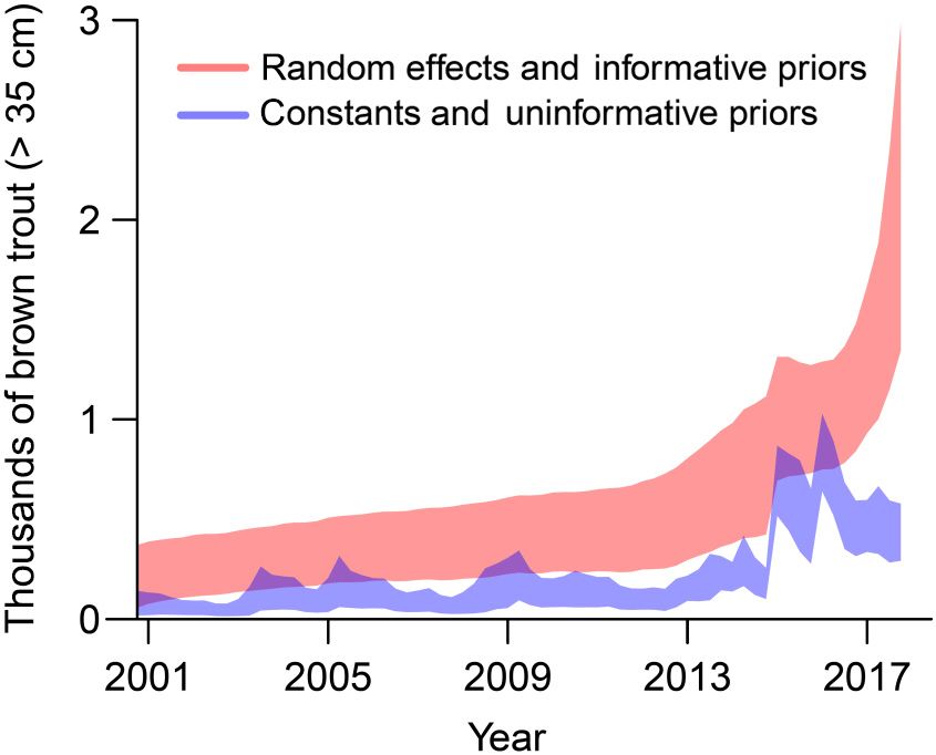
Ecological Applications
Article e02112; page 4                           CHARLES B. YACKULIC ET AL.                                                 Vol. 30, No. 5

TABLE 2. Marginalization approach to discrete latent states.

                                                                                      f: marginalized calculations at each time step
Observed unique capture histories                  Frequency                        t=2                                          t=3

                                                                                  pu                               p u
                                                                                                                    2    2
 111                                                 1
                                                                                 0                                 0
                                                                                  ð1  pÞu
 121                                                 1
                                                                                   ð1  uÞ                         ð1  pÞpu2
                                                                                                                      0
                                                                                  pu
 112                                                 2
                                                                                   0                               pð1  pÞu2
                                                                                                                   puð1  uÞ
 122
                                                                                    ð1  pÞu                            ð1  pÞ2 u2
                                                     6
                                                                                     ð1  uÞ                       ð1  uÞð1 þ ð1  pÞuÞ

  Notes: The 1’s in capture histories indicate that an individual was observed alive, and 2’s indicate that an individual was not
observed. The probability of being in each state is calculated in each time step base on the observed capture history and survival (φ)
and detection (p) probabilities. The overall likelihood of an observation is given by the sum across all states in the last time step and
the log of this likelihood is multiplied by the frequency of a unique capture history and summed across all unique capture histories.

(the first capture history in Y), a likelihood of (1  p)             applications. Next, we fit D and M versions of the
pφ2 for an individual seen only on the second recapture               model in three popular open software programs that
event (the second capture history in Y), pφ (1  φ) + p               share the common BUGS language: JAGS (J; Plum-
(1  p)φ2 for an individual seen only on the first recap-             mer 2003), WinBUGS (W; Lunn et al. 2000), and
ture event (third unique capture histories in Y) and                  OpenBUGS (O; Lunn et al. 2009). We compare the
ð1  uÞ þ ð1  pÞuð1  uÞ þ ð1  pÞ2 u2 for the remain-               speed and output from these six options (JD, JM,
ing capture histories in which individuals were never                 WD, WM, OD, OM) to a seventh option consisting
recaptured. Importantly, because the discrete latent                  of a marginalized version fit in Stan (SM). We stress
states are not actually simulated, it is not necessary to             that marginalization can be applied in various pro-
run identical capture histories multiple times, rather, the           grams and is not a specific feature of the programs
likelihood of a capture history can simply be raised to               we use here.
the power of its frequency (or frequency can be multi-                   D and M code in the BUGS language share a first
plied by the log-likelihood of a capture history).                    block of code in which survival, φt, and capture proba-
                                                                      bility, pt, are given uniform priors between zero and one.
                                                                      In addition, we introduce two arrays defining state tran-
        Application 1: CJS applied to rainbow trout                   sitions, x, and the observation process, q. The first row
                 (Oncorhynchus mykiss)                                in x keeps track of the probability that an individual sur-
   For a more concrete illustration of these different                vives, φt, (i.e., remains in state 1) or dies, 1  φt, (i.e.,
approaches, we next apply a CJS model to real data.                   transitions to state 2). The second row ensures that dead
Data in this application come from a mark–recapture                   individuals remain dead (i.e., the transition from state 2
study of rainbow trout in the Colorado River just down-               to 1 is fixed at 0 and the transition from state 2 to state 2
river of its confluence with the Little Colorado River.               is fixed at 1). The dimensions of this array could easily
Rainbow trout were sampled using electrofishing on 18                 be extended for a multistate mark–recapture model and
quarterly trips between April 2012 and October 2016                   values within the array modified for a dynamic occu-
(for more study details, see Korman et al. 2015, Yackulic             pancy model. The first row of q keeps track of the prob-
et al. 2018b).                                                        ability of being captured (pt) or not captured (1  pt)
   For this application only, we present the code in                  conditional on being alive, whereas the second row
the manuscript text that distinguishes the two different              ensures that dead individuals can only ever be not cap-
approaches to illustrate the minor differences. We                    tured. Again, the dimensions could easily be extended
begin by fully describing code for discrete (D) and                   for multistate models and values defined differently for
marginalized (M) versions of a fully time-specific CJS                different classes of models (e.g., false-positive models).
model in the BUGS language. We then give a brief                      The parameters x and q are defined for each interval, t,
overview of a M version in the Stan language (Car-                    in the set of total intervals, Nint
penter et al. 2017). Stan is an increasingly popular                  for (t in 1 : Nint){
(and faster) open software that does not support dis-                     phi[t] ~ dunif(0,1)
crete latent states. We refer readers to the supplemen-                   p[t] ~ dunif(0,1)
tary material for the full Stan code of this and other                    omega [1, 1, t] = phi[t]
July 2020                           MARGINALIZING DISCRETE LATENT STATES                            Article e02112; page 5

    omega [1, 2, t] = (1 - phi[t])                             time using matrix multiplication to determine the like-
    omega [2, 1, t] = 0                                        lihood of being in each state at time t + 1, given
    omega [2, 2, t] = 1                                        information encapsulated in the f array and the tran-
    rho [1, 1, t] = p[t]                                       sition matrix x, and standard multiplication with the
    rho [1, 2, t] = 1 – p[t]                                   probability of the observation in time t + 1. An
    rho [2, 1, t] = 0                                          important feature of this code is that if an individual
    rho [2, 2, t] = 1}.                                        is observed in time period t + 1 (i.e., y_sum[i, t + 1]
  In the D version, this block of code is followed by a        equals one), then q2,1, the probability of observing a
second block in which Y and Z matrices are specified for       dead individual as alive is zero and thus the overall
each individual, i, and time, t according to                   probability of being in the dead state in that interval
for (i in 1 : NY){                                             becomes zero. Once the code has looped through all
    Z [i, indf [i]] = 1                                        time periods, the likelihood of that individual capture
    for (t in indf [i] : Nint){                                history is then calculated by summing across all possi-
      Z [i, (t+1)] ~ dcat (omega[Z [i, t], , t])               ble states. The final line of the code is a modification
      Y[i, (t+1)] ~ dcat(rho[Z[i, (t+1)], , t])}}              of the “ones” trick in the BUGS language, which
                                                               updates the posterior by the value of the likelihood
where NY is the number of individuals captured one or          raised to its frequency.
more times, Z is a matrix with the discrete latent states         The Stan language differs from BUGS language in
for each individual during each sampling event, Y is a         several ways that have been reviewed elsewhere (Betan-
matrix with capture histories for each individual, indf is     court 2017, Monnahan et al. 2017) and we provide code
a vector specifying the first trip on which each individual    in the supplementary materials, so readers can familiar-
is captured, and dcat refers to the categorical distribu-      ize themselves. However, code for a SM version of the
tion (analogous to the multinomial distribution). The          CJS model differs from the M version presented above
code loops through all the individuals (i.e., from 1 to        in only one substantial way. Namely, the last two lines of
NY). Within each individual, it fixes the latent state, Z,     the M version in the BUGS language are replaced by the
to be alive (i.e., Z = 1) in the first time period they were   following line of code:
observed, and then loops forward through the remaining         target += FR[i] * log(sum(zeta[i, (Nint + 1),]))
time periods, simulating both the process of survival and         which directly adds the log-likelihood of a unique cap-
death (through the Z matrix), and the detection process        ture history to the posterior.
(by comparing the Z matrix to the actual capture history          Different versions of the same model led to indistin-
data found in the Y matrix).                                   guishable estimates of parameter means and quantiles
   In the M version, the first block of code remains the       but varied by almost four orders of magnitude in the
same, but the second block becomes                             time required to produce 100 effective samples of the
for (i in 1 : NS){
                                                               least converged parameter. Discrete versions in JAGS,
    zeta[i, sumf [i], 1] = 1
                                                               WinBUGS, and OpenBUGS took a few hours, while
    zeta[i, sumf [i], 2] = 0
                                                               marginalized versions in the same languages took a few
    for (t in sumf [i] : Nint){
                                                               minutes and a marginalized version in Stan took a few
      zeta[i, (t+1), 1] = inprod(zeta[i, t, ],
                                                               seconds (Fig. 1). Differences in speed between versions
      omega[, 1, t]) * rho[1, y_sum[i, (t+1)], t]
                                                               were attributable to two factors: (1) the degree of auto-
      zeta[i, (t+1), 2] = inprod(zeta[i, t, ],
                                                               correlation in posterior draws, which determined how
      omega[, 2, t]) * rho[2, y_sum [i, (t+1)], t]}
                                                               many iterations were required per effective sample and
      lik[i] = sum(zeta[i, (Nint+1), ])
                                                               (2) the average speed of each iteration. Discrete versions
      fr[i] ~ dbin(lik[i], FR[i])}
                                                               generally led to highly correlated posterior draws requir-
                                                               ing ~200 iterations per effective sample, whereas
   where NS is the number of summarized (unique)               marginalized versions in the BUGS language required
capture histories, y_sum is a matrix with each unique          ~10 iterations per effective sample and the SM version
capture history in Y, FR is the frequency of each cap-         required fewer than 2 iterations per effective sample
ture history, sumf is a vector specifying the first trip       (Appendix S1: Fig. S2). SM was also the quickest ver-
with a capture history for each unique capture history,        sion at producing iterations yielding ~60 posterior sam-
zeta is a three-dimensional array, lik is a vector with        ples per second, whereas the JM yielded ~12 samples per
the likelihood of each unique capture history, dbin            second, and other versions yield 1.5–4.0 samples per sec-
refers to the binomial distribution, inprod refers to          ond. We fit all seven versions over a range of iterations
the inner product of two vectors, and fr has the same          and found our conclusions were insensitive to the total
values as FR. Here the code only cycles through                number of iterations that models were run provided
unique capture histories. For each unique capture his-         models were somewhat converged (Appendix S1:
tory, the code fixes the likelihood of being in the alive      Fig. S1). For the rest of the manuscript, we focus on JD
state to 1 and the likelihood of being in the dead             and JM versions of model as proxies for the other BUGS
state to zero. The code then loops forward through             language versions alongside SM versions. To provide
Ecological Applications
Article e02112; page 6 CHARLES B. YACKULIC ET AL. Vol. 30, No. 5
between size classes and between the LCR and CR. Sur-
vival is assumed to be constant with respect to time, and
growth and movement vary seasonally, but are constant
across years. For more details, we refer readers to the
supplementary materials and previous analyses reported
in Yackulic et al. (2014b).
We attempted to fit these data using JD, JM, and SM
versions of the code; however, the JD version was run
for 20,000 iterations, taking 8.3 d (~700,000 s) and was
still far from convergence (effective sample of 5.6 for
least converged parameter). In contrast, all 10 runs of
the SM version finished 2,000 iterations in less than two
hours, yielding more than 500 effective samples for all
parameters and an average time of ~15 minutes per 100
effective samples of the least converged parameter. JM
was an order of magnitude slower at producing 100
effective samples of the least converged parameter but
was still capable of yielding inferences on the scale of
FIG. 1. Comparison of the speed of seven different versions hours. While this section illustrates the motivation for
of a Cormack-Jolly-Seber (CJS) model applied to rainbow trout marginalizing discrete latent states in a Bayesian frame-
data. Whiskers cover the full range of observed speeds based on work, pragmatists may question why we would not just
10 runs of each version of the CJS model. Speed is measured
as the time per 100 effective samples in the least converged use a maximum likelihood framework, which would be
parameter. even quicker. In fact, Yackulic et al. (2014b) used a max-
imum likelihood approach for this very reason; however,
the assumption of temporally constant parameters is
further illustration of the need for faster Bayesian problematic, and the data are too sparse to fit the fully
population models, we next consider a more complex time-dependent model, thus motivating the use of ran-
model. dom effects. In the next section, we return to this appli-
cation illustrating how random effects can easily be
incorporated into this model to provide inferences that
Application 2: Multistate mark–recapture model applied
are not easy to derive using a classic maximum likeli-
to endangered humpback chub (Gila cypha) in the
hood approach.
Colorado River (CR) and its tributary the Little
Colorado River (LCR)
TO BAYES OR NOT TO BAYES: A PRAGMATIC RESPONSE
This application was the primary motivation for many
of the authors to first explore marginalization in a Baye- In our experience, most ecologists (not to mention
sian framework. We have yet to run a JD version of the stakeholders and resource managers) are not making
model for enough time to reach convergence. The data decisions about whether a Bayesian or maximum likeli-
are sparse and include large numbers of animals that are hood approach is appropriate based on philosophical
marked and never seen again. Data were collected arguments. Rather, choices frequently reflect a variety of
between 2009 and 2017 in both the LCR and the fixed factors, including familiarity with different approaches,
site in the CR. In addition to three spatial states (LCR, features of a given problem, and perceived tradeoffs
CR in the sampled area, CR outside the sampled areas), between the speed of a more complex analysis and the
we considered two size classes referred to as small adults differences in value of inferences to be derived from a
(200–249 mm) and large adults (250+ mm) because of more complex analysis. It is not uncommon to read
differences in the vital rates and detection probabilities manuscripts purporting that a more complex analysis is
of different size adults, leading to a total of six potential better because it more closely mimics the complexity of
“alive” states for adults in the multistate mark–recapture ecological systems without clearly articulating actual
model. We ran our model on a seasonal basis. Biological advantages in terms of inferences. A pragmatic analyst
parameters include size transition (growth) and location does not choose a slower or more complex analysis if it
transition (movement) parameters, as well as survival will give identical, or near identical inferences (although
and a parameter that represents the proportion of adult they might reasonably choose an analysis that is slower
humpback chub found in the CR study area out of the computationally but does not require investing resources
total population of adult humpback chub that live in the in developing new code).
CR and spawn in the LCR. The sampled and unsampled From the perspective of a pragmatic analyst that is
portions of the CR are assumed to have the same sur- familiar with maximum likelihood, there is no reason to
vival, growth, and movement parameters, however, sur- take a Bayesian approach for either of the first two
vival, growth, and movement parameters do differ applications. The priors on all parameters are uniformJuly 2020 MARGINALIZING DISCRETE LATENT STATES Article e02112; page 7
and cover the full range of sensible values (i.e., 0 to 1) so SMRE version of the multistate model). Addition of
a maximum likelihood approach would provide indistin- random effects increased the time to sample 100 effective
guishable parameter estimates. Furthermore, maximum samples by 31% primarily by modestly increasing auto-
likelihood estimation is almost always quicker than even correlation in posterior draws. Addition of random
a marginalized Bayesian approach, and with minimal effects illustrated that the declines in LCR catch were
modifications, the code presented for these applications the result of reduced adult movement into the LCR dur-
can be used to fit via maximum likelihood. However, ing the spawning season in 2015 as opposed to declines
there are benefits to taking a Bayesian approach for in adult survival (Fig. 2A, B). Consistent with this
some applications. In the rest of this section, we explore demographic interpretation, humpback chub catch in
three applications where there is value in taking a Baye- the LCR has recovered in recent years and estimates of
sian approach over a maximum likelihood approach. total adult abundance were stable throughout the study
Specifically, we focus on the added inferential value to period (Fig. 2C).
be gained from random effects and informative priors. In many instances, it is advisable to consider time-
varying fixed effects based on well-reasoned a priori
hypotheses alongside temporal random effects. As an
Revisiting application 2 to make inferences about
example, we included season as a factor in both the
temporal variation in vital rates
growth and movement portions of the humpback chub
In application two, adult humpback chub survival application based on a priori knowledge that these rates
was assumed to be constant and movement and vary substantially by season. When data are sparse, and
growth were assumed to differ seasonally, but to be the uncertainty associated with any given interval is
constant across years. Some authors would refer to high, there is potential for an important aberration in a
this as a model with full pooling of information (or vital rate over one or more intervals to be obscured by
nearly full because of the seasonal differences). pooling if fixed effects are not also included. Using ran-
Attempts to relax these assumptions and estimate dif- dom effects alongside fixed time-varying covariates is
ferent rates for each time interval (a time-dependent also advisable as an approach to deal with the noninde-
parameterization like application 1) would be referred pendence of individuals exposed to the same conditions
to as a complete lack of pooling. For these data, a during a given interval (Barry et al. 2003).
time-dependent parameterization leads to uselessly
imprecise estimates with 95% confidence intervals
Pseudo-R2
spanning essentially from 0 to 1. Random effects rep-
resent an intermediate between these two extremes Use of random effects, alongside fixed effects, also
sometimes referred to as partial pooling (Gelman and allows ecologists to quantify how much of the variation
Hill 2007). With rich data sets (or when the number of in one or many parameters of interest is explained by a
intervals are less than five) random effects models will covariate or series of covariates, by calculating a pseudo-
behave similarly to time-dependent models. With spar- R2 value. This approach differs from an analysis of
ser data and more intervals, however, random effects deviance, which is applied to nested models and focuses
models will behave more like a constant parameter on the overall fit of a model. Calculation of pseudo-R2
model. Benefits of random effects in population mod- values follows from Gelman and Pardoe’s (2006) treat-
els have been recognized for almost two decades (Link ment of multi-level R2. Specifically, the pseudo-R2 for a
1999, Burnham and White 2002, Royle and Link parameter is defined as
2002). While random effects can be included in maxi-
mum likelihood analysis, their application is often not EðvarRE Þ
pseudo R2 ¼ 1
straightforward, especially when random effects are EðvarREþFE Þ
included in more than one parameter of interest. One
advantage of a partial pooling approach is that in where EðvarRE Þ is the expected variance of random
some situations, it can allow us to detect temporal effects across posterior draws and EðvarREþFE Þ is the
changes in vital rates that would be obscured by expected variance of the sum of the random effects and
imprecision in a time-dependent model and assumed all fixed effects across posterior draws. While this
to be nonexistent in a fully pooled model. approach is intuitive, it has not been widely used in the
In the case of humpback chub, a substantial decline in population modeling literature (but see Yackulic et al.
adult catch in the LCR spatial state was observed begin- 2018b). In the humpback chub application, season is
ning in spring 2015 and there were questions about the included as a factor in the equations governing size tran-
degree to which this decline reflected variation in sur- sitions (i.e., growth) in both spatial locations, and there
vival vs. movement rates with implications for the status are four separate movement parameters estimated in
and trend of the overall population. To quantify varia- each interval so we can estimate how much of the tem-
tion in these parameters, we fit a version of the marginal- poral variance in each of these parameters of interest is
ized model in Stan with random effects for survival, explained by season. We calculate pseudo-R2s of 0.79
growth and movement (hereafter referred to as the and 0.92 for movement of small and large adultEcological Applications Article e02112; page 8 CHARLES B. YACKULIC ET AL. Vol. 30, No. 5 FIG. 2. Estimates of (A) movement into the Little Colorado River by large adult humpback chub during the spawning season (spawning rate), (B) annual survival of large adults in the Colorado River, under a model with random effects and a model that assumes constant rates, and (C) total abundance of adult humpback chub that spawn in the Little Colorado River. Lines indicate the 95% credible intervals for estimates from each year given by the random effect model, while the gray polygon represents the 95% credible intervals from a model that assumes a constant rate over time. humpback chub out of the CR into the LCR, and 0.66 and 0.91 of the variance in the LCR. In the next applica- and 0.78 for movement of small and large adult hump- tion, we consider a situation where random effects are back chub out of the LCR into the CR. With respect to used to pool among species in a community as opposed growth, season explains 0.77 of the variance in the CR to over temporal intervals.
July 2020                          MARGINALIZING DISCRETE LATENT STATES                             Article e02112; page 9

  Application 3: Dynamic community occupancy model                Application 4: Informative priors in an integrated
     applied to birds in the Sky Islands of Arizona               population model of brown trout (Salmo trutta)
   Community occupancy models are an extension of                Ecologists do not frequently use informative priors
single-species occupancy models (Dorazio et al. 2006)         intentionally (but see Garrard et al. 2012). Most Baye-
and are commonly applied to data from avian studies           sian population analyses instead choose priors that are
that use point-count sampling (Russell et al. 2009).          believed to be weakly informative or entirely noninfor-
Community occupancy models estimate occupancy, spe-           mative, leading to estimates that are indistinguishable
cies richness, and with multiple time periods, local colo-    from a maximum likelihood approach. This approach is
nization and extinction probabilities, while accounting       problematic in some situations for at least two reasons.
for imperfect detection. Despite the growing popularity       First, seemingly uninformative priors can still affect
of community occupancy models, the slowness of these          inferences (Seaman et al. 2012, Northrup and Gerber
models has led many applications to explore only a lim-       2018) and there is a tendency to not critically evaluate
ited set of potential competing models, and has limited       priors when they are believed to be uninformative (espe-
the scope of simulation studies exploring issues of study     cially if models are very slow). Second, in applied set-
design and biases (but see Sanderlin et al. 2014, Guil-       tings, there are often situations where data are sparse,
lera-Arroita et al. 2019). Here we illustrate how commu-      outside knowledge exists to inform one or more parame-
nity occupancy models can be marginalized using a             ters, and the purpose of the modeling is not to test this
model with multiple years of data in which species’           existing knowledge, but to make predictions or test
detection probabilities are modeled as random effects         hypotheses about other parameters. Under these circum-
and species’ colonization and extinction probabilities        stances, failure to include prior information can lead to
are modeled using random effects that also vary by seven      imprecise or biased predictions and inefficient manage-
habitat types. The complexity of this model is represen-      ment decisions. In this application, we show how priors
tative of commonly applied community occupancy                and marginalization can lead to better, and faster, pre-
models.                                                       dictions to inform a decision-making process motivated
   We apply the model using detection/nondetection            by an increasing invasive species.
data collected for 149 bird species across 92 sites in           Brown trout have been present in the CR system for
the Chiricahua Mountains of southeastern Arizona,             decades; however, catch of brown trout in the river
USA. Each site was visited three times in each of five        segment just downstream of Glen Canyon Dam was
years (1991–1995), with the exception that only 68 sites      low until a substantial increase between 2012 and
were visited in the first year of the study. These data       2017. Stakeholders and resource managers were con-
are a subset of data previously analyzed by Sanderlin         cerned with this trend because brown trout are piscivo-
et al. (2013). To make the example more tractable (but        rous and capable of large movements and a large
still cover the range of bird species that are abundant       brown trout population potentially threatens the popu-
and easy to detect vs. rare and hard to detect), we           lation of humpback chub located downriver. The
selected the largest mountain range in this study, the        model presented here was developed to forecast the
Chiricahua Mountains, and only made inference on              potential consequences of different management
species detected at least once in the original study (i.e.,   actions through a structured process described in
we included species not detected in the Chiricahua            Runge et al. (2018). The model assumes three size
Mountains, but detected in another mountain range).           classes, a seasonal time step, and includes both fixed
For more details concerning the model and data, see           and random effects. The model is fit using catch and
Sanderlin et al. (2013) and the supplementary materi-         effort data collected between fall 2000 and fall 2017
als.                                                          throughout the ~25 km of the Glen Canyon reach of
   JD, JM, and SM versions lead to indistinguishable          the CR, as well as mark–recapture data collected on
estimates of all parameters we monitored. Interestingly,      seasonal trips between spring 2012 and fall 2017 at a
the JM version was the fastest taking an average of           fixed 2-km section within the larger reach. The mark–
17 minutes to reach a minimum of 100 effective samples,       recapture data are sparse, and we realized during
while the SM version took an average of approximately         model development that we would not be able to pro-
37 minutes and the JD averaged over 5 h. When models          vide useful forecasts without utilizing outside informa-
are applied to larger communities, we expect that the rel-    tion in the form of priors. In particular, we used the
ative difference between M and D versions will likely         Lorenzen equation (Lorenzen 2000) and estimates of
increase, particularly, when data include many species        the average length in each size class during each sea-
that are only seen rarely and include many sites. Later in    son, to derive a prior of seasonal and size class-specific
the manuscript we report estimates of species richness        survival rates. Past mark–recapture studies of other
produced by marginalized and discrete versions of this        fish species in the CR have found substantial temporal
model, however, we next consider an example that illus-       variation in capture probability (Korman and Yard
trates how informative priors can be useful when data         2017, Yackulic et al. 2018b), therefore the model uses
are particularly sparse.                                      random effects to allow for temporal variation in
Ecological Applications
Article e02112; page 10 CHARLES B. YACKULIC ET AL. Vol. 30, No. 5
capture probability. Here, we fit four versions of the preferable to have more robust data to base inferences
model, including JD, JM, and SM versions of the on, we were inclined to put more weight on abundance
model with informative priors to compare computation estimates from the SM version since parameter estimates
speed. To illustrate the importance of informative pri- from the SM version made more ecological sense based
ors in this application, we also compare the parameter on our understanding of how survival changes with
estimates from the SM version to an SM version that body size in fish species in general, and based on expec-
replaces the informative prior on survival with an tations for capture probability in a large river such as the
uninformative prior and removes random effects on Colorado River.
capture probability (SM-NPI—No Prior Information).
Parameter estimates derived from SM, JM, and JD
Summary
versions were indistinguishable. The time to reach a min-
imum 100 effective samples averaged 29, 161, and Understanding how to marginalize is useful for applying
193 minutes for SM, JM, and JD versions, respectively. maximum likelihood approaches and improving the speed
Many estimates from SM and SM-NPI versions differed of Bayesian approaches. We generally choose an approach
substantially. For example, the SM-NPI estimated based on the features of a given problem. In this section,
annual survival of brown trout in the largest size class as we have examined some applications for which a Bayesian
0.37 (95% CI: 0.2–0.54), which is substantially lower approach is beneficial. In all three applications explored in
than estimates of rainbow trout survival in the same this section, marginalization increased computational
reach based on more robust data (Korman et al. 2015) speed dramatically, which was important given that use of
as well as the estimate of 0.65 (95% CI: 0.41–0.85) for random effects generally slows models. For application 2,
brown trout in the middle size class. At the same time, we previously showed that a JD version without random
estimates of capture probability from a model without effects failed to converge after 8.3 d, so a random effects
informative priors on survival were greater than for simi- version was only possible through marginalization. In the
lar sized rainbow trout, even though adult brown trout next two sections of the manuscript, we discuss issues that
are known, from unpublished telemetry studies in the are common to both maximum likelihood and Bayesian
system, to spend much of their time at depths that application of marginalization: the recovery of latent states
should make the relative inaccessible to electrofishing and use of auto-covariates.
(R. Schelly, personal communication). Use of informative
priors on survival and addition of random effects to cap-
RECOVERING DISCRETE LATENT STATES: ISSUES AND TERMS
ture probability led to estimates that were more consis-
tent with these observations and also led to very One perceived issue with marginalizing discrete latent
different inferences regarding brown trout population states is that inferences are sometimes focused on the dis-
dynamics (Fig. 3). While it would certainly have been crete latent states. For example, it may be necessary to cal-
culate the probability that a given site is occupied by a
species or estimate the overall abundance of a population.
Before explaining how latent states like these can be
recovered, we begin by defining some general terms. We
introduce the term first-order state to refer to a state at
the scale of the individual or site (e.g., alive/dead, or occu-
pied/unoccupied) and the term second-order state to refer
to a state derived by applying some operation to the first-
order states (e.g., abundance is the sum of alive individu-
als, species richness is the sum of all species occurring in a
site). This distinction is important because if inferences
are focused on second-order states only, it may not be
necessary to recover first-order states, or it may be suffi-
cient to imperfectly recover first-order states.
To clarify what is meant by imperfect recovery, we
must first distinguish between unconditional and condi-
tional estimates of first-order states and further distin-
guish between three different forms of conditional
FIG. 3. Estimates of the abundance of brown trout over
35 cm over time in the Glen Canyon reach of the Colorado estimates. Unconditional estimates do not use specific
River under a model that includes random effects and informa- information from an individual’s capture history or
tive priors or a model that assumes constant rates and uninfor- site’s detection history, relying instead on estimates of
mative priors. Constant models without informative priors parameters (which are themselves informed by all the
suggest a volatile population, but also lead to estimates of other
parameters that are unlikely. Inclusion of random effects and data) and individual or site covariates. A closed (or sea-
informative priors lead to parameter estimates closer to expec- sonal) conditional estimate combines the unconditional
tations and higher abundance estimates. estimate with specific capture/detection information forJuly 2020 MARGINALIZING DISCRETE LATENT STATES Article e02112; page 11
the period of interest; however, it ignores specific cap- to a much simpler expression for the forward conditional
ture/detection information from preceding or subse- estimate
quent time periods. A forward conditional estimate uses
capture/detection information and relevant parameters p Þ2
ð1 be Þð1 b
from the current and all preceding time periods. Last, a ðforwardconditionalÞ
p Þ2 þ be
ð1 be Þð1 b
fully conditional estimate uses the entire capture or detec-
tion history and relevant parameters to determine first-
In other situations, we might also include a (1 p)p
order state probabilities during any period. During the
term to reflect the detection history during the first per-
final period of a capture or detection history forward
iod; however, this would end up in all terms in the
and fully conditional estimates are exactly the same. A
numerator and denominator here and thus would cancel
fully conditional estimate should exactly match esti-
out. Similarly, when we consider the information from
mates derived using discrete latent states (a point we
the third period it is tempting to include a p2 in all terms
illustrate in the next paragraph). All other approaches
to reflect the two detections; however, this would end up
should be imperfect estimators (imperfect in the sense
cancelling out. Instead the only relevant information
that they do not use all the available information). How-
from the full capture history is that the site must have
ever, these other approaches are easier to calculate and
not gone extinct, ð1 be Þ, between the second and third
may be sufficient in many applications.
periods if it was occupied in the second period, or must
To make the distinction between these estimates of
have been colonized, b c , if it was unoccupied during the
first-order states more concrete, consider an imaginary
second period. Taken together this yields the fully condi-
detection history from an occupancy study over three-
tional estimate for the example
time periods with two visits in each period [01 00 11].
We assume that initial occupancy ( w), b colonization (b c ),
extinction (be ), and detection probability (^p) are constant p Þ2 ð1 be Þ
ð1 be Þð1 b
ðfullyconditionalÞ
and previously estimated. We focus here on different p Þ2 ð1 be Þ þ be b
ð1 be Þð1 b c
estimates for the second period. The unconditional esti-
mate for the second period would simply be the proba- Taking the thought experiment a step further, we can
bility the site had been occupied in the first period, w, b calculate these different estimators under different
and did not go extinct, 1 be , during the first interval parameter values and compare them to estimates from a
added to the probability the site was not occupied in the discrete latent state approach (Table 3). Whereas the
first period, 1 w, b and colonized, bc , during the first fully conditional estimate is always equivalent to the dis-
interval crete latent state estimate, the other estimators are differ-
ent and sometimes very different. For the parameter
b ð1 be Þ þ 1 w
w b bc ðunconditionalÞ
values considered here the forward conditional approach
provides better approximations than the closed condi-
Note that this estimate includes none of the specific tional or unconditional approaches.
detection information from any interval (including the More generally, unconditional, closed conditional and
information that we know the site was in fact occupied forward conditional estimates can be calculated easily
during the first interval) and only considers the probability with minimal modifications to the marginalized code
the site was occupied. As soon as we begin to incorporate presented for each application in this manuscript. For
detection history information, we also need to consider example, a forward conditional estimate of being in
the probability the site was not occupied. If we only use state, s, for any individual/site, i, and time, t, can be
information from the second period, the site was either
occupied and was not detected on both surveys with a
b be Þ þ ð1 wÞb
probability of ½ w1 b c ð1 b
p Þ2 or was never TABLE 3. Estimates of occupancy during the second season of
b ð1 be Þþ the three season detection history with two visits per season,
occupied with a probability of ð1 ½ w [01 00 11], vary depending on parameter values and the
b
ð1 wÞb c Þ. We can then calculate the closed conditional approach to estimating occupancy.
estimate by dividing the probability of occupancy by the
w c e p U closedC forC fullC DLS
sum of the probabilities of occupancy and nonoccupancy
0.75 0.6 0.2 0.1 0.75 0.71 0.76 0.81 0.81
b ð1 be Þ þ 1 wb b 0.75 0.6 0.8 0.1 0.3 0.26 0.17 0.06 0.06
½w c ð1 bp Þ2
h i h i 0.75 0.1 0.2 0.1 0.63 0.57 0.76 0.96 0.96
b ð1 be Þ þ 1 w
w b bc ð1 b p Þ2 þ ð1 w b ð1 be Þ þ 1 w
b bc Þ 0.75 0.6 0.2 0.6 0.75 0.32 0.39 0.46 0.46
ðclosedconditionalÞ Notes: We assumed different values for model parameters:
initial occupancy (w), colonization (c), extinction (e), and detec-
Since the site was detected as occupied in at least one tion probability (p), and calculated unconditional (U), closed
conditional (closedC), forward conditional (forC), and fully
survey during the first period, we know the site was in conditional (fullC) estimates and compared them to estimates
fact occupied during the first period and can replace all from a discrete latent state model (DLS). All estimates are
b in the closed conditional equation with 1, which leads
w rounded to two decimal points.Ecological Applications
Article e02112; page 12 CHARLES B. YACKULIC ET AL. Vol. 30, No. 5
fi;t;s
calculated from the array, f as Pj¼S where S is the sets based on either low (p = 0.1) or high (p = 0.5) cap-
j¼1
fi;t;j ture probability and fit each data set using either a JD
total number of states. Deriving fully conditional estimates approach with N-augmentation or a JM approach with
is less straightforward to calculate automatically as it draws from the negative binomial distribution (JM-NB).
involves calculating the likelihood of a particular capture We compared coverage of 50% and 95% confidence
or detection history for every possible sequence of discrete intervals as well as relative bias between the two estima-
latent states. For this reason, it is useful to identify condi- tion approaches. Both approaches had minimal positive
tions when more easily calculated, but imperfect, estimates relative bias (July 2020 MARGINALIZING DISCRETE LATENT STATES Article e02112; page 13
and variances. Here, we focus on comparing estimates autologistic effects can lead to poor inferences and pre-
from JD and JM approaches. Mean estimates of first- dictions, however, estimating the strength of these effects
order states are nearly identical in the final year (R2 of in field settings is not straightforward because estimates
0.999 with minor discrepancies attributable to MCMC of vital rates and second-order states are uncertain and
error) and highly correlated in earlier years (Fig. 4A). typically estimated jointly with non-negligible sampling
When estimates of first-order states from the JM version correlations. In most circumstances, discrete latent state
are summed, point estimates of species richness are simi- approaches provide unbiased estimates of these effects
lar to those derived from the JD version, but uncertainty and it is unclear how to approach such effects if discrete
is underestimated (Fig 4B). Both point estimates and latent states have been marginalized out to improve
variances on species richness are nearly identical pro- speed. In our final two applications, we compare param-
vided binomial trials based on expected occupancy from eter estimates (and speed) between JD, JM, and SM ver-
the JM version are summed (Fig. 4C). sions in which the marginalized versions use forward
conditional estimates to calculate auto-covariates (an
autologistic term in the fifth application and a density-
AUTO-COVARIATES: DO WE LOSE ANYTHING THROUGH
dependent term in the final application). After dis-
MARGINALIZATION?
cussing these applications, we consider other approaches
The general concept that individual vital rates are that have been suggested for calculating second-order
influenced by second-order latent states is ubiquitous in states for use as auto-covariates.
ecological theory and thought to play an important role
in many applied situations. For example, it is often
Application 5: Two-species occupancy model with an
hypothesized that recruitment and/or survival depend
autologistic effect applied to Northern Spotted Owls
on population size, decreasing as the population
(Strix occidentalis caurina) and Barred Owls (Strix
increases and providing a mechanism for population reg-
varia) in Tyee study area in Oregon, USA
ulation. Similarly, it is often hypothesized that rates of
colonization or extinction of different habitat patches or Northern Spotted Owls are threatened by both habitat
territories will depend on the number of already occu- loss and competition with invading Barred Owls (Yack-
pied patches or territories in near proximity (i.e., autolo- ulic et al. 2019). Two-species dynamic occupancy models
gistic effects). Autologistic effects can be based on the have been used to quantify the impacts of competition
proportion or number of occupied patches/territories in and habitat on Northern spotted owl dynamics (Yack-
some neighborhood or by weighting patches or territo- ulic et al. 2014a, Dugger et al. 2016) and autologistic
ries by their distance and/or size. Failure to include pop- effects defining the whole study area as a neighborhood
ulation processes like density dependence and describe temporal patterns in barred owl colonization
FIG. 4. Comparisons of occupancy and species richness estimates between marginalized and discrete versions of a community
occupancy model. (A) Although a few of the 68,540 posterior mean occupancy estimates differ substantially between a discrete (x-
axis) and marginalized (y-axis) version of a community occupancy model, estimates in the final year of the study are almost per-
fectly correlated (with slight discrepancies attributable to MCMC error) and estimates in the first four years of the study are highly
correlated. (B) Summing marginalized estimates of occupancy (y-axis) from each posterior draw within sites to estimates species
richness leads to average estimates that are highly correlated with species richness estimates from a discrete version (x-axis) in the
first four years and almost perfectly correlated in the final year. However, this approach underestimates uncertainty in species rich-
ness estimates by 55% as indicated by the ovals centered on the mean estimates and given radii equivalent to the standard deviation
of species richness estimates from the two versions. (C) Summing binomial draws based on each posterior occupancy estimate from
a marginalized version leads to the same mean expectations and yields standard deviations in species richness that are very similar
(4% greater) to those derived from a discrete approach as indicated by the nearly circular nature of the ovals. Dotted line in each
plot indicates the 1:1 line.You can also read