A Radial Measurement of the Galaxy Tidal Alignment Magnitude with BOSS Data
←
→
Page content transcription
If your browser does not render page correctly, please read the page content below
MNRAS 000, 1–23 (2018) Preprint 22 February 2018 Compiled using MNRAS LATEX style file v3.0
A Radial Measurement of the Galaxy Tidal Alignment Magnitude
with BOSS Data
Daniel
1
Martens1 , Christopher M. Hirata1 , Ashley J. Ross1 , Xiao Fang1
Center for Cosmology and AstroParticle Physics, Department of Physics, The Ohio State University, 191 W Woodruff Ave,
Columbus OH 43210, U.S.A.
arXiv:1802.07708v1 [astro-ph.CO] 21 Feb 2018
21 February 2018
ABSTRACT
The anisotropy of galaxy clustering in redshift space has long been used to probe the rate
of growth of cosmological perturbations. However, if galaxies are aligned by large-scale
tidal fields, then a sample with an orientation-dependent selection effect has an additional
anisotropy imprinted onto its correlation function. We use the LOWZ and CMASS catalogs
of SDSS-III BOSS Data Release 12 to divide galaxies into two sub-samples based on their
offset from the Fundamental Plane, which should be correlated with orientation. These sub-
samples must trace the same underlying cosmology, but have opposite orientation-dependent
selection effects. We measure the clustering parameters of each sub-sample and compare them
in order to calculate the dimensionless parameter B, a measure of how strongly galaxies are
aligned by gravitational tidal fields. We found that for CMASS (LOWZ), the measured B was
−0.024 ± 0.015 (−0.030 ± 0.016). This result can be compared to the theoretical predictions of
Hirata (2009), who argued that since galaxy formation physics does not depend on the direction
of the “observer,” the same intrinsic alignment parameters that describe galaxy-ellipticity
correlations should also describe intrinsic alignments in the radial direction. We find that the
ratio of observed to theoretical values is 0.51 ± 0.32 (0.77 ± 0.41) for CMASS (LOWZ). We
combine the results to obtain a total Obs/Theory = 0.61 ± 0.26. This measurement constitutes
evidence (between 2 and 3σ) for radial intrinsic alignments, and is consistent with theoretical
expectations (< 2σ difference).
Key words: large-scale structure of Universe, cosmology: observations, cosmological param-
eters
1 INTRODUCTION number density in galaxy surveys, which provided greater empirical
evidence for mapping nonlinear effects (Kaiser 1986). The unifor-
Galaxy peculiar velocities have long been known as a source of
mity of the Universe on scales above approximately 100h−1 Mpc
noise in using the redshift of a galaxy to infer its distance from
was seen in tandem with a complicated network of non-linear be-
the observer. When redshift surveys are used to map the large-scale
haviors on smaller scales. While on small scales, RSDs trace the
structure of the Universe, these peculiar velocities leave artifacts
velocity dispersion of the galaxies, the RSD signal on scales large
known as redshift space distortions (RSDs). On small scales, RSDs
compared to the Finger of God length does not become negligible;
lead to “fingers of God” – structures that are smeared in redshift
instead it traces linear-regime infall into potential wells. The distor-
space by their internal velocity dispersion rather than by their phys-
tions on these larger scales can measure the matter density of the
ical size, and hence appear to be pointed at the observer (Jackson
Universe, Ωm , as described in detail by Kaiser (1987). Following
1972). This smearing increases the difficulty of making precise mea-
this, Hamilton (1992) derived formulas to measure Ωm given the
surements in redshift space. However, on large scales, RSDs are also
characteristic anisotropic quadrupole of the correlation function.
on a short list of invaluable cosmological probes. Matter overden-
sities cause infall of galaxies on these scales, which results in a These methods have been applied to increasingly larger sur-
“squashing” effect when viewed in redshift space. Measurements veys, primarily producing measurements for the RSD parameters
on the magnitude of this large-scale infall can reveal information on themselves. Hamilton (1993) applied these to the Infrared Astro-
the clustering of matter in the Universe, even out to linear scales. nomical Satellite (IRAS) 2 Jy, observing 2,658 galaxies, and finding
Early galaxy surveys (Kirshner et al. 1981; Bean et al. 1983) that Ωm = 0.5+0.5
−0.25
. Cole et al. (1995) measured redshift-space dis-
lacked the number density of sources to well quantify the effects tortions for 1.2-Jy and QDOT surveys, and compared their results
of RSDs, as they were limited to a few thousand galaxies, although to N-body simulations to find points of breakdown with linear the-
attempts were made to model them (Davis & Peebles 1983). By the ory, further studied by Loveday et al. (1996) on the Stromlo-APM
1990’s, however, improved spectroscopic techniques led to a higher redshift survey. The optically selected Durham/UKST Galaxy Red-
© 2018 The Authors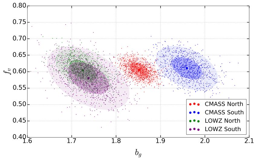
2      Martens et al.
shift Survey pursued similar measurements (Ratcliffe et al. 1998).              In this paper, we use the fundamental plane of elliptical galax-
Within recent years, galaxy samples have become larger, and er-           ies to determine, in a statistical way, which galaxies are intrinsically
rors on measured parameters have become correspondingly smaller.          aligned along or across our line of sight. We then divide the BOSS
Peacock et al. (2001) used the 2dF Galaxy Redshift Survey to mea-         catalogs into subsamples of galaxies in each orientation classifica-
sure redshift-space distortions from 141,000 galaxies, and detected       tion. Our aim is to obtain a measurement of the linear alignment
a large-scale quadrupole moment at greater than 5-sigma signif-           amplitude B using radial alignment measurements, to complement
icance. This result was expanded by Verde et al. (2002) through           existing shear measurements of the same quantity. We perform this
incorporating the galaxy bispectrum to place a measurement on the         analysis using data from the Baryon Oscillation Spectroscopic Sur-
matter density, finding Ωm = 0.27 ± 0.06. Currently, RSD cluster-         vey (BOSS; Dawson et al. 2013), which was observed as part of the
ing measurements serve to test the standard models of the growth          Sloan Digital Sky Survey - III (Eisenstein et al. 2011). Specifically,
of structure. In this endeavor, larger samples of galaxies have been      we use both the “LOWZ” and “CMASS” catalogs (Reid et al. 2016)
analyzed using higher redshift surveys (Ross et al. 2007; Guzzo           from Data Release 12 (DR12; Alam et al. 2015). We divide these
et al. 2008), 6dFGS (Beutler et al. 2012), WiggleZ (Blake et al.          catalogs into two separate populations depending on each galaxy’s
2012), and SDSS and BOSS (Tegmark et al. 2004; Okumura & Jing             estimated orientation relative to us, as assessed using the offset from
2009; Dawson et al. 2013; Chuang et al. 2017; Satpathy et al. 2017;       the Fundamental Plane. Next, we perform clustering measurements
Ross et al. 2017; Gil-Marín et al. 2016; Beutler et al. 2017). RSD        to determine RSD parameters for each group, testing the predictions
measurements have also been conducted for high-redshift Lyman             of this effect by Hirata (2009), and comparing our radial measure-
break galaxies (da Ângela et al. 2005; Mountrichas et al. 2009;           ment of B to a perpendicular measurement using galaxy ellipticities.
Bielby et al. 2013). Finally, results from these analyses have been             This paper is organized as follows. In Section 2, we discuss the
combined with CMB observations (Tegmark et al. 2006; Alam et al.          theory behind the galaxy intrinsic alignments and how they mimic
2017) to measure the full range of cosmological parameters.               redshift space distortions. Specifically, in Section 2.3, we discuss
      As galaxy survey sizes grow and the precision on RSD mea-           the Fundamental Plane, and how we will use it to determine each
surements increases, it is important to keep track of and mitigate        galaxy’s orientation relative to our line of sight. Section 3 describes
potential sources of error. One such source of error, discussed ini-      the BOSS DR12 dataset – both the catalogs themselves, the selection
tially by Hirata (2009), is caused by the intrinsic alignment of galax-   choices we have used for our sample, and our methods of blinding
ies due to large-scale tidal fields. Luminous red galaxies (LRGs),        and systematics tests. We discuss in Section 4 the methods by which
which have been targeted extensively by recent surveys, are pref-         we calculate the clustering statistics on our samples, as well as how
erentially aligned along the stretching axis of the local tidal field,    we generate our covariance matrices. Finally, in Section 5 we discuss
which when combined with observational selection effects based            how we fit RSD parameters to our samples, and analyze the results.
on orientation, results in differences in the observed density modes,     We conclude in Section 6.
depending on if the mode is parallel, or perpendicular to, the line of          Unless noted otherwise, we use the following cosmological
sight. Specifically, a viewing dependent selection effect of observing    parameters: ΩΛ = 0.693, h = 0.68, Ωb = 0.048, Ωm = 0.307,
more galaxies which are pointed toward us can result in an increase       ns = 0.96, σ8 = 0.83, and Tcmb = 2.728 K (Planck Collaboration
in perpendicular k-modes and decrease of parallel k-modes. Hirata         et al. 2014).
(2009) estimates that this effect could result in the contamination
of RSD measurements by 5–10 percent, depending on specifics of
the redshift and mass distribution of the galaxy sample in question.
Related effects have been studied in the context of other galaxy sam-     2     THEORY
ples (e.g. Lyman-α emitters, Zheng et al. 2011; Behrens & Braun
2014) and of higher-order statistics (Krause & Hirata 2011).              2.1    Redshift space distortions
      Intrinsic alignments of luminous red galaxies are correlations      There are two main effects which change the naïve linear power
between their respective orientations, shapes, and physical posi-         spectrum in redshift space. Both of these are due to changes in
tions. The development of these alignments is a complicated, non-         radial velocities of observed galaxies, although the effects differ in
linear process associated with the history of galaxy formation, but       both their sources and their end results. First, peculiar velocities
the payoff for cosmology if they are understood can be huge (Chisari      of galaxies cause a random shift in their observed radial velocity,
& Dvorkin 2013). Proposed alignment mechanisms include linear             with some galaxies moving toward us and others moving away. This
alignment by large-scale tidal fields (Catelan et al. 2001; Hirata &      causes a spread in the observed distribution of galaxies on small
Seljak 2004), large clusters of galaxies (Thompson 1976; Ciotti &         scales, creating an incoherent “Finger of God” effect, where groups
Dutta 1994), or tidal torque contributions to galaxy angular mo-          of galaxies appear to be pointing toward the observer, when viewed
mentum (Peebles 1969). LRGs specifically have had their intrinsic         in redshift space. Although this effect has long been understood,
alignment amplitudes analyzed both in observations (Hirata et al.         a second effect detailing a coherent redshift space distortion was
2007; Bridle & King 2007; Okumura & Jing 2009; Blazek et al.              described by Kaiser (1987). On larger scales, galaxies are pulled
2011; Chisari et al. 2014) and in simulations (Velliscig et al. 2015;     into local gravitational overdensities, leading to a squashing effect
Chisari et al. 2015; Tenneti et al. 2016; Hilbert et al. 2017). Ana-      in redshift space, which is a significant correction to the redshift
lytical models for describing these processes have been developed         space galaxy correlation function, even on linear scales.
and expanded upon (Blazek et al. 2015, 2017). Their effects on                  These distortions affect measurements along the line of sight,
weak lensing has been, so far, the greatest motivation for their study    and so changes to the linear power spectrum are a function of µ, the
(Troxel & Ishak 2015). Intrinsic alignments have been measured us-        cosine of the angle between a given direction and the line of sight.
ing galaxy-galaxy lensing (Mandelbaum et al. 2006; Joachimi et al.        We can write the observed overdensities of galaxies in Fourier space
2011; Huang et al. 2016; van Uitert & Joachimi 2017; Huang et al.         as:
2018; Tonegawa et al. 2017) for the LOWZ sample (Singh et al.
2015) which we compare to in this work.                                   δg (k) = (b + f µ2 )δm (k),                                         (1)

                                                                                                                        MNRAS 000, 1–23 (2018)
Radial Tidal Alignment                     3
where δg and δm refer to perturbations measured by galaxy trac-            alignments and the observational selection effects (we explore this
ers and matter, respectively, b is the linear galaxy bias, and             in more detail below), and si j is the dimensionless tidal field:1
 f = d ln G/d ln a, where G is the growth function. It can be seen
                                                                                                  1
that we recover the matter power spectrum multiplied by the tracer         si j (x) = ∇i ∇ j ∇−2 − δi j δm (x).                               (5)
bias if we are looking at modes transverse to the line of sight. This                             3
equation can also be expressed as the relationships between the            This leads to a modified equation for the power spectrum:
matter and galaxy tracer power spectra:
                                                                                                       2
                                                                                          A
Pg (k) = (b + f µ2 )2 Pm (k)                                        (2)    Pg (k) = b − + ( f + A)µ2 Pm (k).                                         (6)
                                                                                          3
It is common to measure the amount of anisotropy by the parameter
β = f /b.                                                                  This equation, although within the confines of the assumptions we
                                                                           have made, is powerful. We have introduced a single parameter, A,
                                                                           to describe the effects of intrinsic alignment upon redshift space
2.2    Intrinsic alignment effects on RSD measurements                     distortions. Note that the functional behavior of the distortions re-
                                                                           mains the same, but the intrinsic alignments have shifted the usual
Hirata (2009, hereafter H09) showed that systematic errors to red-         parameters in the model. Therefore, any systematics tests aiming
shift space distortion measurements can occur through the intrinsic        to filter out effects of a different functional form will not be able
alignment of galaxies by large scale tidal fields. It requires two con-    to sift out this specific type of contamination. In the presence of
ditions to be met for the galaxy sample in question. First, galaxies       intrinsic alignment effects, the usual RSD measurement of f can
must be intrinsically aligned along the stretching tidal field axis        be re-interpreted as a measurement of f + A, with the “standard”
(“linear alignment” in the nomenclature of intrinsic alignment the-        assumption being that A is small.
ory). Second, the sample must have a selection effect that depends               In order to extract specifically the tidal alignment effect, we
on the galaxy orientation relative to the line of sight. The systematic    need to factor A into pieces that depend on the observational se-
error in f depends on the product of these effects. In this paper,         lection effects (over which we have some control) and pieces that
we are deliberately enhancing the selection effects by splitting the       depend on intrinsic alignments (which we seek to measure). This
BOSS sample into subsamples using a proxy for orientation. This            means we need a mathematical description of the intrinsic align-
enables us to use the difference in inferred f from the subsamples         ments. Following H09, we treat elliptical galaxies as a triaxial sys-
to probe intrinsic alignments.                                             tem which is optically thin. For any position s from the center of
      It can be seen in a physical sense how alignments can lead to        the galaxy, the volume emissivity is j(s) = J(ρ), where ρ is the
these systematic effects by understanding their resulting changes to       ellipsoidal radius, and is defined by:
observed Fourier density modes, as shown qualitatively in Figure
1. The anisotropic selection has a different effect on density modes       ρ2 = s · exp(−W)s.                                                        (7)
depending on the angle of the mode with the line of sight directional
                                                                           Here W is a 3 × 3 traceless-symmetric matrix that contains infor-
vector. Selection of galaxies which are aligned perpendicular to
                                                                           mation on the anisotropy of the galaxy, and J(ρ) specifies the radial
the line of sight of the observer leads to a further decrease in the
                                                                           profile.2 For a spherical galaxy, W = 0. The radial alignment is en-
amplitude of troughs in k-modes perpendicular to the line of sight,
                                                                           coded in W33 (with positive W33 for a prolate galaxy pointed at the
which serves to amplify those k-modes. Conversely, this selection
                                                                           observer), whereas the sky-projected alignments relevant for weak
will lead to a decrease in the amplitude of peaks in k-modes parallel
                                                                           lensing are encoded in W11 − W22 and 2W12 .
to the line of sight, resulting in a smoothing of these k-modes. This
                                                                                 Note that real elliptical galaxies cannot generally have ho-
anisotropic effect mimics clustering signals by amplifying modes
                                                                           mologous iso-emissivity contours since this does not explain the
in different ways along the line of sight than transverse to it. This is
                                                                           well-known isophote twist (see §§4.2.3 and 4.3 of Binney & Mer-
the “physical picture” which serves to illustrate how redshift-space
                                                                           rifield 1998 for an overview). This could lead to a difference of the
distortion measurements can be biased high or low, depending on
                                                                           alignment parameters measured by different techniques (e.g. Funda-
the galaxy selection effect in question.
                                                                           mental Plane offset versus ellipticity). However we expect the effect
      To describe this effect quantitatively, we give a quick synopsis
                                                                           of intrinsic alignments to still be present, and qualitatively similar
of the analysis of H09 and highlight the results needed for under-
                                                                           to the homologous case.
standing LRG clustering (we refer the reader to H09 for additional
                                                                                 In the linear tidal alignment model, we take the first order
details on the formalism). We denote the contribution of anisotropic
                                                                           approximation in the Taylor expansion of hWi j i in the tidal field:
selection effects to the galaxy overdensity by  – that is, the observed
number density of galaxies at point x as seen from direction n̂ is         hWi j i = 2Bsi j .                                                        (8)
taken to be 1 + ( n̂| x) times the number density that would be ob-
served if the galaxy orientations were randomized. At linear order,        This leads to

                                                                           A = 2(η χ)eff B,                                                          (9)
δg (k) = (b + f µ2 )δm (k) + (ê3 | k),                            (3)
where we take the convention that the observer’s line of sight is the
3-axis.
                                                                           1  Since si j is traceless-symmetric, it follows mathematically that  (n̂ |x)
      In the linear tidal alignment model (relevant for LRGs), the         averages to zero if we average over viewing directions n̂.
                                                                           2 H09 worked only to linear order in W, and Sec. 5.1 of H09 defined ρ with
intrinsic alignments trace the large-scale tidal field:
                                                                           (I + W)−1 instead of exp(−W). For an observational paper working with real
( n̂| x) = Asi j (x)n̂i n̂ j ,                                     (4)    galaxies, we need to handle higher orders in W; the definition in Eq. (7) is
                                                                           more convenient as the total luminosity of the galaxy extrapolated to ρ = ∞
Here A is a biasing parameter, which depends on both the intrinsic         is independent of W.

MNRAS 000, 1–23 (2018)
4       Martens et al.

                                                                                            W33 Positive

                                                   Observer                                 W33 Negative                         Observer
Figure 1. Here we show an exaggerated situation demonstrating a selection bias having an anisotropic effect on the resulting k-modes. If we assume that our
observations are less likely to observe galaxies which are aligned perpendicularly to our line of sight, then some of the galaxies visualized above will not appear
to the observer (the crossed-out galaxies). Since galaxies are more likely to be aligned with the higher density modes of the gravitational field, this changes the
measured k-modes of the observed galaxies. Fourier modes perpendicular to the line of sight will have deeper troughs, and thus a higher inferred amplitude,
while k-modes parallel to the line of sight will have shallower peaks, and thus a lower inferred amplitude. In this work, we intentionally group galaxies by their
orientation, shown here by the color of green or blue. If we were to view all of these galaxies, but were less likely to see galaxies of the ‘’‘blue” type, then these
distortions would dampen the linear Kaiser effect of clustering in our observation. (Note: this figure is similar to Figure 1 of Hirata (2009), but adapted to the
situation with two sub-samples.)

where                                                                                 2.3    Sub-samples using the Fundamental Plane offset
             ∂(ê3 | x) ∂ ln Ngal                                                    The Fundamental Plane (FP) relation for elliptical galaxies was ob-
(η χ)eff =              =                                                 (10)
             ∂W33 (x)     ∂W33                                                        served by Djorgovski & Davis (1987), who noticed an empirical
                                                                                      relationship between a galaxy’s luminosity, radius, and projected
is the selection-dependent conversion factor from W33 (radial galaxy
                                                                                      velocity dispersion. Increasingly detailed measurements of these
orientation) to observed number of galaxies.3 Here again it is seen
                                                                                      correlations have been made (Jø rgensen et al. 1996; Bernardi et al.
that A is only non-zero if we have both non-random orientations
                                                                                      2003a; Hyde & Bernardi 2009) and there are good theoretical argu-
B , 0 and an orientation-dependent selection effect (η χ)eff , 0.
                                                                                      ments for its existence (Bernardi et al. 2003b). We use the redshift
      The parameter B can be compared to other parameters for the
                                                                                      and luminosity of our observed galaxies in tandem with the FP re-
linear intrinsic alignment model used in the literature, such as bκ
                                                                                      lation to estimate each galaxy’s radius4 . This radius can then be
(Bernstein 2009), where
                                                                                      compared to the radius fit by the SDSS imaging pipeline to es-
        B                                                                             timate the galaxy’s orientation, through use of the estimator W33
bκ =        .                                                             (11)
       1.74                                                                           (referenced in Section 2).
      We can also compare to the lensing measurements AI of Singh                           The key idea is that from our vantage point we do not observe
et al. (2015) (derived in Appendix B):                                                the full 3-dimensional galaxy, but a 2-dimensional projection. In the
                                                                                      case of an optically thin galaxy (as for most LRGs), this is simply
                Ωm
B = −0.0233          AI
                                                                                                ∫
                                                                          (12)
                G(z)                                                                  I(s ⊥ ) =    j(s ⊥ + s3 ê3 ) ds3 .                             (13)
where Ωm is the matter density and G(z) is the redshift-dependent
growth function.
                                                                                      4  We do not use the velocity dispersion information, for several reasons.
                                                                                      The velocity dispersion is dependent upon what axis our line of sight takes
3 In H09, a simple flux threshold was assumed, with various definitions               through the given galaxy, which complicates our assessment of orientation-
for the flux of an extended object considered. In this case, one could write          dependent offsets from the Fundamental Plane. Moreover, the BOSS fibers
A = 2η χB, where η is the slope of the luminosity function and χ depends              do not sample the whole galaxy, and we have not explored the subtle correla-
on how fluxes area measured for non-spherical objects. In this paper, we              tions that might be imprinted when this effect couples to orientation effects
implement a more complicated selection algorithm, but we can still think of           and observational conditions. We avoid these issues entirely, at the cost of
the conversion factor as an “effective” η χ.                                          some extra statistical error, by fitting for only the redshift and luminosity.

                                                                                                                                         MNRAS 000, 1–23 (2018)
Radial Tidal Alignment                    5
The projection of a homologous triaxial galaxy gives an image with
an effective radius5 :

             1         1 2
re = exp − W33 − (W13      + W23
                               2
                                  ) + ... res,                (14)
             4         4
where res is the effective radius for the spherical galaxy (W = 0).
With this knowledge, we can use Eq. (14) to construct an estimator
for W33 , accurate to linear order:
                re
  obs
W33   = −4 ln      .                                           (15)
               re0
where we have distinguished the true value of W33 from the linear-
order approximation, which we define as W33     obs . For the rest of the
paper, we will refer to the linear-order quantity as W33 in order to
simplify notation; however, it must be understood that it contains
both measurement noise and noise from intrinsic scatter in the FP
relationship. Here, re is the effective radius as measured by BOSS,
and re0 is the value of the radius found using the FP. The combination
of these measurements gives us an estimate for each galaxy’s W33                 Figure 2. For the CMASS samples, we chose to fit Eq. 16 separately to
value, and hence each galaxy’s orientation.                                      galaxies in ranges of 0.43 < z < 0.5, 0.5 < z < 0.6, 0.6 < z < 0.65,
      Specifically, we find an estimate of the isotropic average size            and 0.65 < z < 0.7. This helped mitigate an observed correlation between
from each galaxy by fitting a simple linear model over all galaxies              galaxy redshift and median W33 for the CMASS sample. In this plot we
in the survey for the relation between the logarithmic size and the              compare to the same equation fit over the full redshift range of 0.43 < z <
intrinsic magnitude, as well as the galaxy’s redshift:                           0.7 (‘single redshift bin’). Here we show the resulting change in median W33
                                                                                 value by binned redshift for the CMASS SGC sample.
log10 (re0 ) = C1 Mr s + C2 z + C3,                                      (16)
where re0 is the isotropic average size, Mr s is the rescaled galaxy             account for two other parameters, bg and σFOG 2     (a real-space clus-
absolute magnitude (to be defined in Eq. 26), and z is the red-                  tering amplitude and Finger of God length parameter), in order to
shift, while the C values are the parameters fit to the model. We                accurately reproduce the correlation function. These are described
fit this model using the Levenberg-Marquardt algorithm (Leven-                   in more detail in Sections 5.1 and 5.2.
berg 1944) from the Scipy curve-fit algorithm (Jones et al. 2001).                     We now outline the central idea of this paper. We split a parent
With this model, we estimate each galaxy’s angle-averaged size,                  galaxy sample into two sub-samples, using a proxy for orienta-
and hence its orientation, which allows us to separate our catalogs              tion (in this case, offset from the fundamental plane); we expect
into orientation-divided subsamples. For the CMASS sample, it was                the different subsamples to have different values of (η χ)eff . We
found that this fitting procedure resulted in a redshift-biased result           next compute the difference between the redshift space distortion
for W33 , as shown in Fig. 2. Specifically, higher redshift galaxies             amplitudes fv = f + A measured from the two sub-samples. This
were more likely to have fitted radius re0 > re , and therefore a                difference should cancel out the dependence on the true rate of struc-
more negative W33 value. This implies a change in the slope of the               ture growth (via f ); there should also be some cancellation of the
fundamental plane relation with respect to redshift for our CMASS                non-linear effects (though this may not be perfect if the sub-sample
sample. We dealt with this by using four redshift bins in the CMASS              splitting is sensitive to galaxy properties other than orientation, and
sample: 0.43 < z < 0.5, 0.5 < z < 0.6, 0.6 < z < 0.65, and                       these properties are correlated with large-scale environment).
0.65 < z < 0.7. Within each redshift bin, we fit to Eq. (16), which                    Using Eq. (6), we can see the effect that galaxy samples with
helped to mitigate the redshift bias. For the LOWZ sample, we also               different values of A will have on the power spectrum. Specifically,
fit to Eq. (16), but for the entire redshift range, 0.15 < z < 0.43.             separate samples of galaxies, with different values of W33 , will
Once all W33 values were set, we then subtracted the median value                theoretically have different values of A, but the same value of the
for both the LOWZ and CMASS samples, and identified a galaxy’s                   growth function, and thus the same fv . We can therefore find the
inferred orientation by the sign of its W33 value.                               difference in A between samples as
                                                                                 ∆A ≡ A2 − A1 = ( f + A2 ) − ( f + A1 ) = fv,2 − fv,1,                  (17)
2.4   Redshift space distortions of sub-samples
                                                                                 where fv,X indicates the measurement of fv for sample X. Note
In this paper, we primarily fit for the RSD parameter f + A that is              that the “measured” value of the bias (from a fit to the correlation
present in our two sub-samples (split based on a proxy for orien-                function) is actually
tation); the difference ∆( f + A) = ∆A is independent of the linear                         A
rate of growth of structure f , and isolates the anisotropic selection           bmeas = b −  .                                            (18)
                                                                                            3
effects. This is the key parameter of our study; however, we also
                                                                                     From our measurement of ∆A we can then calculate B:
                                                                                                           1 ∂Ngal−      1 ∂Ngal+

                                                                                 ∆A = 2∆(η χ)eff B = 2              −                   B, (19)
5  For an elliptical image, we define the effective radius as the geometric                              Ngal− ∂W33   Ngal+ ∂W33
mean of the semi-major and semi-minor axes of the half-light ellipse. This
                                     2 [exp W]
ellipse has a second moment matrix res         proj , where “proj” denotes the
                                                                                 where a subscript of “+” indicates the group where W33 is greater
2 × 2 sub-block of a 3 × 3 matrix; see the appendix of H09 for a discussion      than the median value (galaxies are brighter/smaller than predicted
of projections. Equation (14) is the Taylor expansion of the square-root-        by the fundamental plane) and a subscript of “−” indicates the group
determinant of this second moment matrix.                                        where W33 is less than the median value (galaxies are dimmer/larger

MNRAS 000, 1–23 (2018)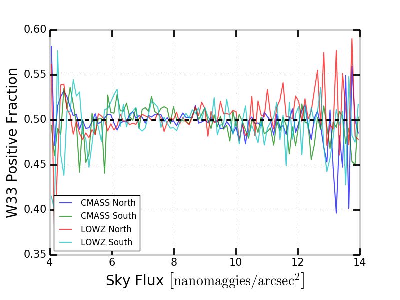
6      Martens et al.
than predicted by the Fundamental Plane). Throughout this paper,             linear alignment parameter AI , to our measurement:
any sign of the difference in parameters, such as ∆ fv , indicates the                     Ωm
value in the “−” group minus the value in the “+” group. While               B = −0.0233        AI ,                                          (21)
                                                                                           G(z)
A depends on how well our sample splitting procedure traces ori-
entation, this dependence is removed when considering B, which               where Ωm and G(z) are the matter density and growth function
depends only on galaxy type and redshift.6 For our sample splits,            at a given redshift for their specific parameter choices, which are:
we have calculated the values of ∆(η χ)eff to be −1.111, −1.100,             Ωm,Singh = 0.282 and G(0.32) = 0.869. Therefore we can calculate
−1.515, and −1.438 for CMASS NGC, CMASS SGC, LOWZ NGC,                       that the lensed measurement for the intrinsic alignment magnitude
and LOWZ SGC respectively.                                                   of the LOWZ sample is:
                                                                             Bpred = −0.0348 ± 0.0038.                                        (22)

2.5   Theoretical expectations                                               Using the same method, we calculate H09’s prediction for the L/L0
                                                                             values found in Singh et al. (2015), which is 0.95. This leads to a
One of the foundational principles in cosmology is statistical ho-           theoretical prediction of −0.029 ± 0.010. All of these predictions
mogeneity and isotropy. In the context of intrinsic alignments, this         are compared to our final results in Section 5.
means that the intrinsic alignment parameters that relate the radial
tidal field s33 to the radial alignment W33 are the same as those that
relate the plane-of-sky tidal fields (s11 − s22, 2s12 ) to the plane-of-
                                                                             3     SURVEY DATA
sky alignment (W11 − W22, 2W12 ). That is, the measurement of how
strongly a galaxy’s alignment is affected by its tidal field should not      3.1    Sample definition and characteristics
depend on whether we measure it radially, as in this work, or in the
                                                                             Our data is taken from the completed and publicly available SDSS-
plane of the sky, as is done in lensing studies. We explore this con-
                                                                             III (Eisenstein et al. 2011) BOSS (Dawson et al. 2013) Data Release
cept in our comparison to theory, and previous literature. The caveat,
                                                                             12 (DR12; Alam et al. 2015) LOWZ and CMASS catalogs. The
of course, is that given practical observational limitations the radial
                                                                             purpose of BOSS was, through measurements of large scale galaxy
and plane-of-sky measurements may not be measuring exactly the
                                                                             clustering, to determine the scale of baryon acoustic oscillations and
same thing. Possible issues include non-homologous isophotes (but
                                                                             hence constrain the cosmic distance scale. Using spectroscopic red-
with a pipeline that assumes a homologous profile); dust extinction;
                                                                             shift measurements, it recovered the three-dimensional distribution
selection effects for the parent samples; and non-linear response
                                                                             of approximately 1.4×10⁶ galaxies, with an effective area of 10, 000
(i.e. higher-order terms in Eq. 14). Plane-of-sky measurements may
                                                                             square degrees. Here, we describe the observations that produced
depend on their own set of assumptions; see Singh et al. (2015);
                                                                             the BOSS data and the general properties of BOSS galaxies.
Troxel & Ishak (2015) for details.
                                                                                   BOSS objects were selected for spectroscopic observation
      We directly compare our CMASS and LOWZ measurements
                                                                             based on SDSS-I/II/III imaging data in five broad bands (ugriz)
of B to that obtained by Singh et al. (2015), who use correlations of
                                                                             (Gunn et al. 2006; Doi et al. 2010). SDSS I/II (York et al. 2000)
galaxy shapes in the plane of the sky. Singh et al. (2015) performs
                                                                             made use of photometric pass bands (Fukugita et al. 1996; Smith
this measurement for the SDSS DR11 LOWZ sample, which we
                                                                             et al. 2002; Doi et al. 2010), imaging roughly 7606 deg2 in the
can directly compare to our DR12 LOWZ sample.
                                                                             Northern galactic cap (NGC) and 600 deg2 in the Southern galac-
      As a further comparison, we can calculate the theoretical in-
                                                                             tic cap (SGC), data of which was released in DR7 (Abazajian
trinsic alignment strength as predicted in Hirata (2009), given a
                                                                             et al. 2009). For DR8, an increased area of the SGC was surveyed
luminosity value for the sample in question. H09 finds that, using
                                                                             (3172 deg2 ) (Aihara et al. 2011). The full SDSS DR8 dataset in-
catalogs of luminous red galaxies:
                                                                             cludes “uber-calibration”, which updates the photometric calibra-
                                   1.48±0.64                               tions within SDSS (Padmanabhan et al. 2008).
                                   L
B = (1.74)(−0.018 ± 0.006)                     ,                    (20)           Spectroscopy was obtained for BOSS targets using the BOSS
                                  L0
                                                                             spectrograph (Smee et al. 2013). Still in operation, it simultaneously
where L is K + e-corrected to z = 0 and L0 is the corrected r-band           obtains 1000 spectra in a given observation. Using the reduction
absolute magnitude of −22. Our r-band absolute magnitudes are                pipeline described in Bolton et al. (2012), redshifts were classified
listed in Table 2. Using the tables provided by Wake et al. (2006),          from BOSS spectra with statistical errors from photon noise at a
who formulate star evolution on models from Bruzual & Charlot                few tens of km s−1 .
(2003), we find that our K + e-corrected r-band median absolute                    The LOWZ sample selects bright, red objects using the specific
magnitudes are −22.17 for LOWZ and −22.295 for CMASS. We                     color-cuts and r-band flux limit defined in Reid et al. (2016). Over
then find that the ratio L/L0 referenced in Eq. (20) is 1.170 for            the redshift range 0.2 < z < 0.4, the sample is nearly volume-
LOWZ, and 1.312 for CMASS. This results in a prediction of B                 limited, with a constant space density of ≈ 3 × 10⁻⁴ h3 Mpc−3 .
equal to −0.039±0.010 for LOWZ, and −0.046±0.011 for CMASS.                  LOWZ galaxies reside in massive halos, with a mean halo mass of
With these values, we can compare our results to that expected by            5.2 × 10¹³ h−1 M (Parejko et al. 2013). In our sample, we applied a
H09.                                                                         cut to galaxies outside of the range 0.15 < z < 0.43, since galaxies
      We can also compare the ellipticity-based measurement of               sufficiently far outside of the target redshift range are more likely
Singh et al. (2015) to that predicted by H09 for their measurement           to be mis-assigned objects. This cut also follows the procedure
of L/L0 . We will use the following equation (derived in Appendix            adopted first in Anderson et al. (2012) and subsequently in other
B) to compare values from Singh et al. (2015), who measure the               BOSS analyses studying the CMASS and LOWZ sample separately.
                                                                             This makes the two samples more independent by avoiding overlaps
                                                                             in redshift range. Further details on the properties of the LOWZ
6  As discussed in Sec. 2.2, there are other conventions for the intrinsic   sample can be found in Parejko et al. (2013); Tojeiro et al. (2014);
alignment amplitude that are related to B.                                   Kitaura et al. (2016).

                                                                                                                         MNRAS 000, 1–23 (2018)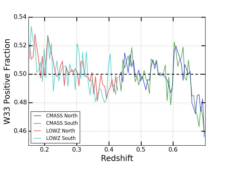
Radial Tidal Alignment                     7
      The CMASS sample applies the specific color cuts and i-band        Vaucouleurs radius, while a ratio smaller than one appropriately
flux limit defined in Reid et al. (2016) in order to provide a sample    scales our fit radius to treat highly elliptical galaxies. The values of
with a number density that peaks at 4.3 × 10⁻⁴ h3 Mpc−3 at z = 0.5       abDev for our samples are listed in Table 2. We next use the spectro-
and is greater than 10−4 h3 Mpc−3 within the range 0.43 < z < 0.65.      scopic redshift from the CMASS and LOWZ tables to calculate the
The selection was designed to obtain a stellar-mass limited sample,      comoving angular diameter distance D to each galaxy. With these
regardless of color (Reid et al. 2016). This results in a sample         distances, we found the size of the galaxy, parameterized by the
of galaxies that are approximately 75% red in color (e.g., Ross          physical half-light radius:
et al. 2014 and references there-in) and elliptical in morphology
(Masters et al. 2011). The majority (∼ 90%) of the galaxies are          s = Dreff .                                                                (25)
centrals, living in halos of mass ∼ 1013 h−1 M (White et al. 2011).
In our sample, we applied a redshift cut to galaxies outside the range   There is a separate size for each galaxy in each band; our analysis
0.43 < z < 0.7, again following the procedure of Anderson et al.         uses the i-band sizes, and perform our fits using log10 size. The
(2012), and again to make the samples independent.                       SDSS database does not include extinction correction, so we apply
      The BOSS footprint is divided into two distinct North and          that here, following the maps of Schlegel et al. (1998), as provided
South Galactic cap regions, which we refer to as NGC and SGC.            by the BOSS catalog; we do not perform any K-corrections (Hogg
These regions have slightly different properties, as described in the    et al. 2002), except when we compare our results to theoretical
appendix of Alam et al. (2017) and references there-in. Thus, we         expectations in Section 5.
analyze the NGC and SGC separately throughout our pipeline, for                We calculate the rescaled absolute magnitudes using:
both LOWZ and CMASS. This yields a total of 4 samples for which
                                                                         Mr s = m + 5 − 5 log10 D A = M + 10 log10 (1 + z),                         (26)
we will obtain results.
                                                                         where Mr s is the rescaled absolute magnitude, M is the absolute
                                                                         magnitude, m is the observed magnitude, and D A is the angular
3.2   Data preprocessing                                                 diameter distance 7 . We perform redshift cuts specific to each survey,
Separate from our cosmological parameters are the set of galaxy          restricting LOWZ to 0.15 6 z 6 0.43 and CMASS to 0.43 6 z 6
parameters which describe measured quantities of each specific           0.70. There is a clear cutoff in the redshift space distribution of
galaxy. The galaxy parameters used in our pipeline fall into two         each survey where the color cuts creating the survey were designed
general categories. The “science” parameters, specifically right as-     to limit the galaxies. However, specifically with the low side of the
cension (RA), declination (Dec), redshift (z), and de Vaucouleurs        CMASS survey, there are “trailing” galaxies which have escaped
fit parameters (magnitudes and radii), are used both in calculat-        the color cuts. We make these redshift cuts for two reasons. First,
ing the orientation parameter W33 and in finding the multipoles of       eliminating these galaxies removes galaxies that were not intended
the correlation function. These parameters are critical to the pur-      to be included by the color cuts, and prevents outliers in redshift
pose and results of this project. All other parameters we refer to       space from dominating our fit. Galaxies on the fringes of the redshift
as “null” parameters. These parameters are not used directly for         distribution could have properties which tend to group them within
science, but are used to trace possible observational systematics        the same orientation subdivision, which would then represent a
that could impact the clustering results, and are not related to the     potential systematic error in the sub-sample clustering analyses.
intrinsic parameters of any specific galaxy. They are the airmass,       Second, the redshift cuts we perform are generally made across the
Galactic reddening E(B − V), sky flux, and point-spread function         literature for clustering analyses of CMASS and LOWZ to which
(PSF) full-width half-maximum (FWHM). We will describe our use           we compare (Ross et al. 2017; Gil-Marín et al. 2016; Chuang et al.
of these null parameters in the Section 3.4.                             2017).
      This section details our use of the science parameters to cal-           At this point, we have values for the size, rescaled absolute
culate the value of W33 for each galaxy. It is important to note that    magnitude, and redshift of each galaxy. We can then begin the
for many of our science parameters (and null parameters), we are         processes described in Section 2.3 for finding galaxy orientations
able to use values specific to each band, whether it be u, g, r, i       for a specific galaxy, with respect to our point of observation. Table
or z. We found that the fundamental plane method had the best-fit        1 shows the number of galaxies in each subsample and the number
results within the i-band, and that the i and r bands both had the       removed due to redshift cuts. The medians and standard deviations
smallest deviation from the FP fits. Thus, we used the i-band for        of the galaxy parameters for each sample, once cut by redshift, are
all variables in our analysis. Beyond band choice, there is also the     shown in Table 2.
choice of which radius estimator to use. The de Vaucouleurs radius
r of a galaxy is found by fitting the surface brightness, I, to:

I(R) = I0 e−7.669 (R/r) −1 ,
                       1/4
                                                                 (23)    7  We originally intended to use the absolute magnitude M here, but at a
                                                                         late stage discovered that this is what was implemented within the pipeline,
where I0 is the surface brightness at the de Vaucouleurs radius (de      which we have called the rescaled absolute magnitude. The rescaled absolute
Vaucouleurs 1948). This law is a specific case of a general Sérsic       magnitude differs from that using the absolute magnitude M by an added
profile, with a Sérsic index of n = 4. We modify the measured radius     factor of 10 log10 (1 + z). This should not make any substantial difference
by incorporating the asymmetry of elliptical galaxies; we convert        in our group selection; the difference in the magnitude will be primarily
from the fitted de Vaucouleurs radius to an effective radius, using:     absorbed into the fit coefficients, with a 1.4% (0.5%) z-dependent change in
            p                                                            the value of C3 for CMASS (LOWZ) in Eq. (16). We tested this change by
reff = rdev abDev,                                               (24)    comparing groups with a radial magnitude assignment to those constructed
                                                                         with radial distance in Eq. (26), and found less than 0.3% difference between
where rdev is the de Vaucouleurs radius and abDev is the ratio of        the definitions of the groups. Note that in the absence of a K-correction, the
the short elliptical axis to the long elliptical axis, again measured    multiples of log10 (1 + z) are essentially arbitrary as they correspond to a
using the de Vaucouleurs fit. A ratio value of 1.0 returns the de        different slope of the spectral energy distribution that defines the zero-point.

MNRAS 000, 1–23 (2018)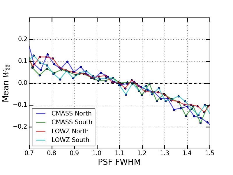
8 Martens et al.
Table 1. Redshift cut statistics for the BOSS CMASS/LOWZ subsamples.
Category CMASS NGC CMASS SGC LOWZ NGC LOWZ SGC
Initial Galaxy Count 618,806 230,831 317,780 145,264
Redshift Cut (%) 8.08 9.71 21.88 21.85
Remaining Galaxies 568,776 208,426 248,237 113,525
S/N 30.389 26.679 83.583 74.306
Table 2. CMASS and LOWZ medians and standard deviations for both the W33 –divided and total samples. Note that the median of W33 for the full samples is
zero by construction.
Statistic W33 > 0 W33 < 0 Total Sample
CMASS sample
Redshift 0.537 ± 0.065 0.546 ± 0.066 0.541 ± 0.063
Absolute Magnitude (r-mag) −22.184 ± 0.317 −22.180 ± 0.307 −22.182 ± 0.310
Apparent Size (log10 kpc) 1.089 ± 0.168 1.328 ± 0.169 1.213 ± 0.206
abDev 0.669 ± 0.178 0.698 ± 0.175 0.684 ± 0.175
W33 0.956 ±0.843 −1.000 ±0.905 0.000 ±1.438
LOWZ sample
Redshift 0.315 ± 0.073 0.319 ± 0.072 0.317 ± 0.075
Absolute Magnitude (r-mag) −22.520 ± 0.385 −22.516 ± 0.337 −22.518 ± 0.399
Apparent Size (log10 kpc) 1.117 ± 0.141 1.300 ± 0.163 1.206 ± 0.172
abDev 0.735 ± 0.169 0.734 ± 0.183 0.747 ± 0.166
W33 0.700 ±0.865 −0.793 ±0.637 0.000 ±1.217
3.3 Sample splitting by orientation
In order to reduce systematic errors in evaluating the W33 component
of each galaxy, it is necessary to accurately reflect the redshift
evolution of the fundamental plane within our sample. We fit all the
LOWZ galaxies with a single fit as described in Eq. (16). For the
CMASS samples, in order to better adjust for changes in the FP due
to redshift, we fit this model separately by several bins of redshift.
We used four redshift bins of 0.43 < z < 0.5, 0.5 < z < 0.6,
0.6 < z < 0.65, and 0.65 < z < 0.7. We found that this scheme
resulted in galaxy samples with orientations as seen in Fig. 3. We
plot the distributions of W33 in Fig. 4.
Once values of W33 were calculated for each galaxy in our
catalog, we then subtracted the median W33 from each galaxy, and
divided our catalogs into two separate samples, depending on the
sign of their W33 value. Galaxies with negative W33 are larger
than we would predict by using the FP method, and we presume
that statistically these galaxies are aligned perpendicular to our
line of sight. Conversely, galaxies with positive W33 are smaller
than we would estimate from the FP method, and we presume that
statistically these galaxies are aligned parallel with our line of sight. Figure 3. For each sample, we show the fraction of positive W33 as a
Although on a galaxy-by-galaxy basis there are other effects which function of binned redshift. Note the good agreement of each distribution
could cause a galaxy to appear bigger or smaller, these effects should across the entire redshift range. For the LOWZ samples, this was achieved
cancel out when measuring ∆ fv for the full sample, assuming that by using the model within Equation 16. For the CMASS samples, it was
these effects are not correlated with the true value of W33 and that necessary to fit this model separately to galaxies in ranges of 0.43 < z < 0.5,
all galaxy sub-samples have the same true value of f . 0.5 < z < 0.6, 0.6 < z < 0.65, and 0.65 < z < 0.7.
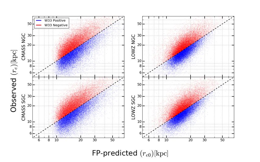
In Figure 5, we compare the photometrically (i-band) measured
size of each galaxy to predicted size based on each galaxy’s redshift
and luminosity, using the FP relationship. We plot 25, 000 randomly Our primary concern with systematic errors is that some pa-
chosen galaxies from each sample, with a line displaying an exact rameter related to observation will leak into our estimates of W33 ,
match between the predicted and observed galaxy size. Our samples and then imprint the spatial structure of the observational effect onto
of positive and negative W33 are defined based on the relationship our sub-samples. For example, if galaxies observed at higher air-
of these parameters. mass have fainter measured magnitudes, then this would offset them
MNRAS 000, 1–23 (2018)Radial Tidal Alignment 9
Figure 4. Here, we plot the histograms for each survey’s distribution of W33 .
from the fundamental plane (they would look “too large” for their surement of intrinsic alignments. However, we want to be sure that
magnitude and their measured W33 would be biased low). In Fig. the differences in clustering properties of the sub-samples are as-
6 we plot the mean W33 value in bins of airmass. For an unbiased sociated with the targets galaxies themselves, and not due to excess
measurement of W33 , we would expect this to fluctuate around zero, clustering imprinted by observational systematics. We do this by
as it should be uncorrelated with the airmass. The effect of seeing intentionally injecting our orientation measurement with a depen-
on the observed galaxy number density has been previously docu- dence on different systematic effects, and compare the resulting
mented in Ross et al. (2017), and could lead to a systematic effect parameters with the intrinsic uncertainty in our true signal. This
in our measurement. Specifically, in the target selection algorithm, section discusses these tests, as well as associated blinding proce-
the distinction between stars and galaxies can be more blurry in dures.
situations of bad seeing. As seeing gets worse, the smallest galaxies First, for what we call Phase I, in Section 3.4.1 we explain
(large W33 values) would be more likely to be labeled as stars, and our random division of samples in order to estimate the amount
less likely to appear in the galactic sample. This cut is related to parameters can vary in samples that have no differences in W33 .
the comparison of the model and PSF magnitudes of the object in There is no specific blinding procedure required at this stage, since
question, and is explained in detail in Reid et al. (2016); Ross et al. we are not computing any clustering properties based on the real
(2011). In Fig. 7, we plot the fraction of galaxies with positive W33 sub-sample split (based on W33 ).
value in bins of sky flux. In Table 3 we display the slope of a lin-
Next, in Section 3.4.2 we describe our injection of systematic
ear fit between the W33 value and four potential systematic effects:
effects into the splitting criteria for W33 . This is still considered a
airmass, extinction, sky flux and the FWHM of the point spread
part of Phase I, since there is again no need to blind the output fit
function. A full quantitative treatment of these systematics and how
parameters, because the values of W33 are internally shuffled before
they influence our results is given in Section 3.4.
being placed in a group. In order to begin Phase II, we require
consistency in the χ2 of the fits with our full samples and null
samples, as well as final parameter offsets that are consistent with
3.4 Systematics tests, random splits, and blinding procedures zero, to indicate that systematics are not imitating the effects of W33
The treatment of systematics is an important aspect of this project. splitting.
We aim to split our sample by the W33 values of each galaxy, and to We enter Phase II in Section 3.4.3 by discussing the fitting of
attribute differences among samples as evidence for a radial mea- our true W33 -based sample division, while blinding ourselves to the
MNRAS 000, 1–23 (2018)10 Martens et al.
Figure 5. For each sample, we use relations of the Fundamental Plane to fit an assumed galaxy radius, based on galaxy luminosity and redshift. Here we plot
this assumed radius to the ’true’ galaxy radius which has been measured photometrically in the i-band. Galaxies are assigned into bins of positive and negative
W33, based on whether their fit radius is greater or less than their measured radius.
true difference in fv . We must be careful here, when checking our
samples for errors, to only display combinations of parameters that
are independent of the final ∆ fv measurement. The parameter com-
bination p(∆bg, ∆ fv ) which achieves this requirement is described
in Section 3.4.3. We also carry out several tests in Phase II for
whether differences in the Finger of God properties of the subsam-
ples could bias our measurement of ∆ fv ; in these tests, only absolue
values of relevant parameters are revealed, so that we remain blind
to the direction of any possible correction. In order to finish our
calculation and fully un-blind ourselves for Phase III, we require
consistency in both samples of this parameter combination, as well
as consistency in the χ2 /dof of the fits.
3.4.1 Phase I: Random Splitting
As described in Section 2, we want to accurately measure B, and
therefore ∆A, for our samples which are separated based on galaxy
alignment. We first need to estimate the statistical error in ∆A, by
measuring the differences in parameters that can occur due to ran-
Figure 6. Here we show the average W33 value, binned by the PSF FWHM. dom sample selection alone. In order to achieve this, we create 500
There is a clear correlation between the PSF FWHM value and a galaxy’s random splits of each survey, and measure the standard deviation of
calculated W33 value. This will be analyzed in more detail in Section 3.4. ∆A, that is: σ∆A. We then compare parameter differences for true
Further evidence of this can be seen in Table 3. samples to this value, to decide if true results are significant or if
systematic effects need to be mitigated. Blinding is not necessary
MNRAS 000, 1–23 (2018)Radial Tidal Alignment 11
Table 3. Values of mθ , for each combination of survey and systematic.
Survey Airmass Extinction Sky Flux PSF FWHM
CMASS South −0.039 0.409 −0.007 −0.331
CMASS South −0.103 0.359 −0.011 −0.255
LOWZ North 0.011 0.232 0.001 −0.261
LOWZ South −0.069 0.318 −0.004 −0.219
However, even this method is prone to statistical errors. The
scrambling step is equivalent to a random assignment of W33 values
to galaxies, and this random assignment step could result in a pa-
rameter shift that has nothing to do with our injected signal, instead
dominated by random fluctuations. To beat down these statistical
errors, we take two steps. First, we perform the random scrambling
step multiple times, so that a true systematic error will become more
evident, while statistical fluctuations will tend to cancel out. Sec-
ond, for each random assignment realization, we perform a “mirror”
realization where the random groups are the same, but we use the
Figure 7. For each sample, we show the fraction of galaxies with positive conversion W33 → −W33 before using Eq. (27). This helps to beat
W33 as binned by the sky flux at the time of observation. Note that there down statistical errors even more quickly, as a given realization
is no obvious correlation between the sky flux on the night of observation, and its mirror will mostly cancel each other’s statistical fluctuations
and the calculated W33 value. Toward the edges of the range we can larger without affecting each other’s biased parameter shift. We perform
deviations from the center, which is due to smaller numbers of galaxies 20 realizations for each null-test, each with their own mirror real-
observed with those values of sky flux.
ization, resulting in 40 total realizations.
in Phase I, as we have not divided the sample in any meaningful 3.4.3 Phase II: fv Blinding
way, and thus the parameters we are measuring are not affected by
intrinsic alignments. As a final test, we disable the scrambling mechanism above, and
fit for the true divided samples. However, we blind ourselves to the
sample values of fv . Instead, we will view the parameter combina-
3.4.2 Null parameter scrambling tion which we call p(∆bg, ∆ fv ):
We continue Phase I by examining potential systematic effects in 1
p(∆bg, ∆ fv ) ≡ ∆bg + ∆ fv, (28)
more detail. For this step, we do not inject any random parameter 3
values for blinding purposes; however, at one point during this test, where ∆ fv and ∆bg indicate the differences in the growth parame-
we scramble the W33 measurements so that they are uncorrelated ters and biases for a sample pair. As can be seen from Eq. (6), this
with their original galaxies, thus destroying any relations between parameter is independent of our offset due to orientation (it does
W33 and the local tidal field for any particular galaxy; therefore, not depend on ∆A). We also would like this parameter to be uncor-
additional blinding protocols at this stage are not necessary. As related with the fv fit for the sample. To test this, we calculated this
discussed above, our list of null parameters includes measurements correlation for all random separations we performed. The results
of airmass, extinction, sky flux and the FWHM of the point spread are displayed in Fig. 8. We can see that there is a non-zero corre-
function. lation value, varying (depending on the sample) between −0.1 and
For each survey and null parameter, before we perform any −0.16. However, as this correlation results in small changes in fv
scrambling, we fit a line to a scatter plot between W33 and the when compared to the random sample separations (see Section 5.4),
specific null parameter θ. From this linear fit, we find the slope of and this step is only necessary to blind ourselves, not find a final
the line, mθ . Ideally, if there is no dependence of W33 on this null uncorrelated result, we believe that this parameter will be effective
parameter, then mθ ≈ 0. The values of mθ are listed in Table 3. Next, as a check at this blinding stage.
we scramble the W33 values randomly among galaxies, destroying During Phase II, we also run several tests to establish that the
any real signal information for blinding purposes. To each galaxy, Finger of God length is not different enough between the subsam-
we modify the scrambled W33 value to become: ples to affect our measurements of ∆ fv . These tests consist fitting
W33 ⇒ W33 + mθ (θ param − θ̄ param ), (27) our final samples for a smaller range of scales at 20–40 Mpc and
2 2
reporting |∆(σFOG )|, and also attempting to measure |∆(σFOG )|
where θ̄ param is the median value of that parameter within the full via direct integrals of the correlation function. They are described
sample. This effectively injects the correlation signal with the null in detail as part of Section 5.2. Note that only absolute values of
parameter into the W33 signal. By fitting each sample set for clus- sub-sample differences are revealed in these Finger of God tests, so
tering parameters, we find a measurement of ∆A, which represents that the direction of any correction (were we to attempt one) is not
the potential spurious value if our estimate of W33 is contaminated revealed.
by the null parameter in question, θ. Ideally, we want this difference In order to pass this stage, and move on to the unblinded
to be much less than the statistical errors on our test measurements final results of Phase III, we require consistency in the samples
of ∆A. for this parameter combination p(∆bg, ∆ fv ), and consistency in the
MNRAS 000, 1–23 (2018)You can also read