An Artificial Intelligence-Based Smart System for Early Glaucoma Recognition Using OCT Images - IGI Global
←
→
Page content transcription
If your browser does not render page correctly, please read the page content below

International Journal of E-Health and Medical Communications
Volume 12 • Issue 4 • Bi-Monthly 2021

An Artificial Intelligence-Based
Smart System for Early Glaucoma
Recognition Using OCT Images
Law Kumar Singh, Department of Computer Science and Engineering, School of Engineering and Technology, Sharda
University, Knowledge Park III, Greater Noida, India & Department of Computer Science and Engineering, Hindustan
College of Science and Technology, Mathura, India
     https://orcid.org/0000-0002-7073-6852

Pooja, Department of Computer Science and Engineering, School of Engineering and Technology, Sharda University,
Knowledge Park III, Greater Noida, India
Hitendra Garg, Department of Computer Engineering and Applications, GLA University, Mathura, India
Munish Khanna, Department of Computer Science and Engineering, Hindustan College of Science and Technology,
Mathura, India

ABSTRACT

Glaucoma is a progressive and constant eye disease that leads to a deficiency of peripheral vision and,
at last, leads to irrevocable loss of vision. Detection and identification of glaucoma are essential for
earlier treatment and to reduce vision loss. This motivates us to present a study on intelligent diagnosis
system based on machine learning algorithm(s) for glaucoma identification using three-dimensional
optical coherence tomography (OCT) data. This experimental work is attempted on 70 glaucomatous
and 70 healthy eyes from combination of public (Mendeley) dataset and private dataset. Forty-five
vital features were extracted using two approaches from the OCT images. K-nearest neighbor (KNN),
linear discriminant analysis (LDA), decision tree, random forest, support vector machine (SVM) were
applied for the categorization of OCT images among the glaucomatous and non-glaucomatous class.
The largest AUC is achieved by KNN (0.97). The accuracy is obtained on fivefold cross-validation
techniques. This study will facilitate to reach high standards in glaucoma diagnosis.

Keywords
Cup Diameter, Cup-to-Disc Ratio (CDR), Decision Tree, Disc Diameter, Glaucomatous, Internal Limiting
Membrane (ILM) Thickness, KNN, LDA, OCT, Random Forest, Retinal Pigmented Epithelium (RPE), SVM

1. INTRODUCTION

Glaucoma is the second most crucial optic ‘eye’ disease in this world. As per sources in 2010,
approximately 60 million populations cross-sectional to be disease infected, and this count is increasing
above 20 million in the period 2020. It does no repairable damage to the central part of the optic
nerves that can lead to making the person blind. Hence, sensing Glaucoma during the initial stage is
very imperative. Generally, doctors focus on the area of the optic disc & optic cup and find the edges
though optic nerve examination. They assure the glaucoma presence they identify the increased size
of the optic cup. One of the essential features is to identify the ratio of the height of the Cup to the

DOI: 10.4018/IJEHMC.20210701.oa3
This article, published as an Open Access article on April 23rd, 2021 in the gold Open Access journal, the International Journal of Informa-
 tion and Communication Technology Education (converted to gold Open Access January 1st, 2021), is distributed under the terms of the
   Creative Commons Attribution License (http://creativecommons.org/licenses/by/4.0/) which permits unrestricted use, distribution, and
          production in any medium, provided the author of the original work and original publication source are properly credited.

32
International Journal of E-Health and Medical Communications
                                                                            Volume 12 • Issue 4 • Bi-Monthly 2021

disc; this is the crucial indicator for identifying Glaucoma. Among the patients, if the Cup-to-Disc
ratio (CDR) value is at least 0.5, it may be considered as the glaucomatous eye.
     Human eye mainly has three layers. The outer layer: Sclera, which is used to protect the eyeball;
Second layer: Choroid and the innermost layer: Retina.”Retina” is liable in vision because of the
presence of photoreceptors. Researchers have invented many techniques which are used for detecting
retinal disorder. These techniques include fundus photography, fluorescein angiography, and the OCT.

Figure 1. OCT image with macular edema

1.1 Optical Coherence Tomography
OCT stands for optical coherence tomography, which is having the property that it is a noninvasive
diagnostic technique used for manufacturing or producing the view of the retina in a cross-sectional
way (Burgansky-Eliash et al., 2005).OCT imaging technology uses OCT cameras, which have low
coherence interferometers in which the low coherence visible light is always allowed to penetrate
the entire human retina and it reflects interferometer producing a cross-sectional image of the retina.
Low coherence of lightning is used for producing images of resolutions—the basic principles of the
OCT imaging technique on the (Michelson type interferometer). A considerable benefit of the OCT
imaging system (Fig. 1) is always that it can detect retinal disorders earlier than other techniques.
     It has been observed that the majority of the work, to date, accomplished by the researcher’s
fraternity is performed on fundus images for glaucoma detection. However, we have used OCT images
as there are multiple advantages of OCT images over fundus images. OCT has higher sensitivity
than the fundus image for the detection of early Glaucoma. It is a non-invasive technology and has a
higher ability to detect small changes in the subretinal layer than the fundus image. This image picks
up the earliest signs of diseases. OCT evaluates disorders of the optic nerve and changes to the fibers
of the optic nerve. It detects changes caused by Glaucoma.
     Moreover OCT(Khalil et al., 2014) images also have higher resolution.OCT provides topographical
information about retinal ganglion cells and Retinal Nerve Fiber Layer (RNFL) abnormalities.OCT
images allow for direct visual analysis of the scans, much the way MRI scans are analyzed, rather
than depending entirely upon computer-driven summary statistics. It can produce real-time a cross-
sectional image of an object, i.e. a two-dimensional image in the space.OCT images give more accuracy

                                                                                                              33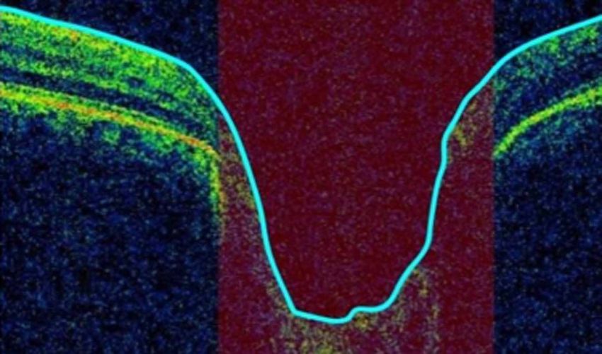
International Journal of E-Health and Medical Communications
Volume 12 • Issue 4 • Bi-Monthly 2021

as compared to the fundus images. Analysis of OCT is done by the degradation of a separate layer,
which increases the efficiency of an image.OCT provides detailed structural information on clinical
abnormalities. This method has been extensively applied to the setting of ophthalmology; this method
is popular due to its ability to perform high-resolution cross-sectional imaging and diagnosing the
changes in the structure of the eye during the progression of this disease.

1.2 OAG - Open Angle Glaucoma
The ordinary form of Glaucoma is open-angle Glaucoma (Fatima et al., 2017). It contrasts the angle-
closure red Glaucoma in which the drainage angle among the cornea and the iris becoming closer;
it blocks fluid from the eye and results in a significant rise in the pressure.
     In Glaucoma (Fig. 2), the decay of fiber nerves causes cup size to increase, and as resultant,
the CDR also increases. CDR is one of the main clinical indicators involved in glaucoma diagnosis.
Accuracy of cup diameter is directly proportional to the Internal Limiting Membrane (ILM) layer,
as CDR is our main feature. That’s why we have extracted the ILM layer. Accuracy of disc diameter
is directly proportional to the RPE layer, as CDR is our main feature; this motivates us to extract the
RPE layer. We have selected the OCT images as subject while major prior published studies have
experimented on fundus images.

Figure 2. Real Image of Glaucomatic Eye

1.3 Motivation and The Proposed Work
Glaucoma is also called silent theft of sight, which results in the irreversible vision loss due to damage
in the optical nerve of an eye. The only available alternative is the early and timely diagnosis of the
disease so that the proper treatment can be started so as to slow down the progression. Ophthalmologist
diagnoses this disease using a retinal examination of the dilated pupil. They use different comprehensive
retinal examinations such as ophthalmoscopy, tonometry, perimetry, gonioscopy and pachymetry to
diagnose glaucoma. But all these approaches are manual, time-consuming and may be prone to
subjective errors. Highly experienced and expert Ophthalmologists are required for precise diagnosis
which leads to the overburden. This all motivates the researcher’s fraternity to develop a fast, accurate
and automated approach in the field of medical imaging for analysis of the retinal images for glaucoma
diagnosis. With the intrusion of techniques like machine learning in the domain of medical imaging,

34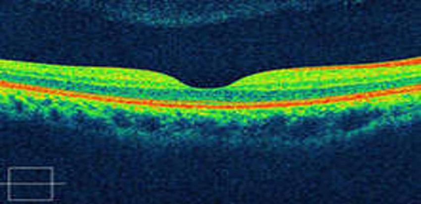
International Journal of E-Health and Medical Communications
                                                                            Volume 12 • Issue 4 • Bi-Monthly 2021

enormous modifications have been observed in the classical techniques of diagnosis of diseases like
glaucoma. The proposed empirical study is a generic attempt to develop robust and highly predictive
machine learning based computer-aided diagnosis system that may aid as an assistive measure for the
initial screening of glaucoma for diagnosis purposes by classifying the retinal images as “healthy”
or “glaucomatous”. 40 ORB features and 5 well accepted vital features are selected for this work to
classify the retinal OCT images of potential patients. The proposed system could serve as a second
opinion for ophthalmologists and at the same instant it will also reduce burden on already overloaded
experienced ophthalmologists and will help humanity.
      The machine learning system had an excellent ability to work on medical imaging classifications.
This inspires us to build a proposed system which will support to enhance the standards for glaucoma
diagnosis and improve diagnosis consistency. We have extracted five features Retinal Pigment
Epithelium (RPE) layer, ILM Layer, Cup Diameter, Disc Diameter, and CDR ratio by self crafted
algorithms and the remaining forty features were extracted using the ORB algorithm. In this empirical
study, additional experiments were performed to validate the system for comparison, we also extracted
OCT parameters and among these parameters average thickness, CDR ratio was calculated.
      These self crafted five algorithms for extracting features from the OCT image are easy to
understand and implement. The quality of the image does not cause any effect on our algorithm; they
still compute an accurate result.
      Going through various search engines we have identified the research gap in this domain, as
per the best of the author’s knowledge, very few reputed studies are recently (or may be in past also)
published on glaucoma identification using OCT images, with the support of machine learning based
classifiers. Hence we are the front runners to propose such a type of, first, study with OCT images,
these forty-five parameters, and the selected five benchmarked machine learning algorithms.
      The organization of this paper is started with the introduction of the type of disease in retinal
(eyes) along with the differentiation of normal eye and Glaucoma infected eye. A detailed description
of OCT and various shortlisted machine learning are also presented. Further, Section 2 discusses the
background and related work in the field of Glaucoma OCT images. In Section 3, a brief outline is
provided for the proposed methodology and various feature extraction techniques required for the
diagnosis of Glaucoma in retinal OCT. Section 4 reports the performance measurement of different
machine learning algorithms for the mentioned purpose along with result discussion followed by the
conclusion at the last Section 5.
      The significant contributions of this paper include the following purpose and objective:

•   To propose the procedures for extracting various features like – RPE, ILM layer, Cup Diameter,
    Disc Diameter, and CDR ratio from the OCT image and thereafter performing experiments
    using these features.
•   Filling up the research gap by proposing the first study, of its own kind, where the objective is
    categorization of OCT images into two separate classes; in which machine learning algorithms
    accept input as values of 45 vital features extracted from OCT images.
•   To provide a comparative study of the simulated results when experiments were performed on
    customized dataset.
•   To perform the prediction of glaucoma with classification accuracy of SVM, KNN, Random
    Forest, LDA, and Decision tree as 75%, 97%, 88%, 92%, and 92%, respectively.
•   Encouraging findings are observed that the KNN model gives the best performance based on
    the accuracy, sensitivity and specificity of the classifier, as 97%, 100% and 85.71%, respectively.

                                                                                                              35
International Journal of E-Health and Medical Communications
Volume 12 • Issue 4 • Bi-Monthly 2021

2. LITERATURE SURVEY

For this section, we have shortlisted some of the prominent prior published studies, including latest
ones, where researchers have attempted to solve the problem in hand. Finally, a comparative table is
also presented for readers.
     Khalil et al.,2018 experimented on SD-OCT images; they have used ILM (inner limited
membrane) as a parameter which gives accurate results even in the poor visualization. They use the
ILM process to generate solid contour that is used to generate accurate cup diameter. In this study, a
technique has been proposed to examine the retinal layer thoroughly for accurate results, it provides the
latest approach to contract with the sharp cases. Practitioners (Pavithra et al.,2019) in their study have
used SD-OCT for the diagnosis of prime open-angle Glaucoma & normal Glaucoma by considering
macular thickness, ganglion cell complex and RNFL thickness .The learning of the neural network
is done in such a mode that the ANN would be able to detect so many glaucoma parameters in all
different levels using the training process. The proposed model was built-up with the help of a feed-
forward backpropagation network in the neural network domain. Authors (Fathima cs et al.,2010)
suggest that Fundoscopy and OCT are the best options for glaucoma detection. Through this, they
calculate the Cup to disc ratio. Researchers have applied K-mean clustering and Otsu thresholding.
     Practitioners (Amina Jameel and Imran Basit,2018) in their empirical study, give a fully automatic
and simultaneous method by utilizing domain knowledge and inexpensive computational methods to
segment 5 layers from an OCT image. Fuzzy histogram hyperbolism is used to transform the distinct
ROI to improve the homogeneity within individual layers. They select the unique hyper-reflective
layers of the retina, which are integrated into the continuous max-flow graph cut framework for
robust segmentation to compute the desirable data term. Anushika Singh et al., 2019 attempted for
detection of Glaucoma, where automated image analysis was developed using wavelet features from
the segmented optic disc. The proposed algorithm was the way of glaucoma recognition that contains
an analysis of wavelet features in the segmented optic disc image.
     In this study (Lee et al.,2018) the Otsu’s thresholding is used as the conversion of greyscale
images into the binary images. This method mainly takes the images in only the two groups of pixels
and it follows the bi-modal histogram method (foreground and background pixel). The calculation
of threshold for optimization in which they separate these into two groups so that their mutual result
extends is equal or can be minimized and also their inter-class variance is high.
     In the experimental study, by Won et al.,2016, the Gray Scale Image (GSI) of all the green
channels are using the CDC process of ILM-layers extractions. The ILM-layer iteration processing
needs to apply for boosting the ILM layer on Gray Scale Image. After that, the thresholding process
is applied to segments retinal layers through all scale images. All the top profiles in the segmented
retinal layer had computed to extract the ILM layer. Next, the ILM layer peak Surface (TSILM)
should be refined by using the set of future novel techniques. At last, the cup edge has placed in
the developed top profile based on the endpoint of the RPE-layer. The study by (Bizios et al.,2010)
uses both ganglion cell inner plexiform layer and retinal nerve fiber layer patterns of glaucoma
progressions by determination using SD-OCT guided progression analysis software. In this empirical
study, by Wollstein et al.,2005 OCT is used as the powerful tool which is used for Glaucoma with
both qualitatively & quantitatively and targeted the optic disc & macular area, it can be reveal pre-
perimetric glaucomic eyes with high sensitivity & specificity. It calculates the retinal nerve fibre
layer thickness and ganglion complex cell thickness.
     This study, Bussel et al., 2014 uses the technology to detect optic disc boundary and for this
purpose image preprocessing is introduced. Initially, the localization of the region of optic disc is to
be presented by using the red channels. These red components have been utilized like it is established
to have the big difference among all the non optic disc & optic disc areas in comparison with the other
channels. For the removal of the blood vessels, the morphological closing operations have been done.
In this study, An et al.,2019 Retinal Nerve Fiber Layer, Optic Nerve Head and Macular thickness are

36
International Journal of E-Health and Medical Communications
                                                                             Volume 12 • Issue 4 • Bi-Monthly 2021

measured for detecting Glaucoma in OCT. ROC curve and sensitivities were calculated . Combination
of RNFL and ONH (Optic nerve hypoplasia) proved to be the best parameter.In the research paper, by
Koh et al., 2018, OCT was used for the glaucoma diagnosis and screening of glucomatic progression.
The commonly available iterations of OCT technology, spectral domain (OCT), have advantage in the
glaucoma assessments. In this authors have presented a number of commercially existing SD-OCT
devices with different parameters and the distinctive features.
     In this next experimental study researchers, Anusorn et al.,2013 observed that the fuzzy logic
and image processing algorithms is a novel expert scheme for early detection of Glaucoma. An
experimental result shows the proposed method superiority. It is mainly based on segmentations of
OD(optic disc) and OC(optic Cup) which is also presented for the identification of Glaucoma and
the segmentation is perform by the use active contour mode.
     Chakraborty, 2019 proposed an automated computer-aided chronic wound diagnostic system
for wound tissue characterization precisely which can address a large volume of patients. Fuzzy
c-means clustering along with four different computational learning schemes viz., Naïve Bayes, Linear
discriminant analysis, Decision tree, and Random forest, have been presented to achieve automated
wound tissue identification for pressure and diabetic ulcer diagnosis. The random forest approach
provided the highest classification accuracy when classifying wound patterns with color features
extracted from the segmented portions of image data sets. In the another study by the same author,
Chakraborty, 2019, analyzed a set partitioning in hierarchical tree (SPIHT) compression technique
for chronic wound image transmission under smart phone-enabled Tele-wound network system. The
proposed system aids in heavy volume of best quality wound images to be compressed, processed
and sent over wireless media with very low bandwidth and reliable networks.
     In very recently published two studies on glaucoma; in first study authors (shehryar et al., 2020)
focused on detection of glaucoma by combining and correlating fundus and SD-OCT image analysis.
In the second study the authors(Ajest et al., 2020)attempted to increase the accuracy of glaucoma
detection by proposing a novel an effective optimization-driven classifier. The proposed Jaya-CSO
is designed by integrating the Jaya algorithm with the chicken swarm optimization (CSO) technique
for tuning the weights of the RNN classifier.
     In this final selected study practitioners, Hassan et al.,2015 observed that Retinal nerve fiber
layer and fast retinal nerve fiber layer is used as a parameter and for the proposed methodology visual
field testing used considering RNFL to differentiate between healthy and glaucomatous eye, and the
result shows that both the parameters gives same accuracy.
     Given below Table 1 presents the detailed description of 13 shortlisted prior published literatures
(some of the studies are recently published) on the basis of various parameters like dataset size,
technique used, scan region selected, accuracy etc.

3. PROPOSED METHODOLOGY

3.1 Objective of This Study
Glaucoma is the most common disease that leads to vision loss (CS,2019). This disease harms the
optic nerve of the eye, and it causes ultimate blindness. It raises intraocular pressure which results
in the increment of Cup to disc ratio if it is not treated at an early stage. The imperative intention of
this study is to search for a methodology to explore and identify Glaucoma during the early stage.
In the scarcity of glaucomatous experts, and automatically Glaucoma detected system, the proposed
system is advantageous.
     As the initial step of the preprocessing stage, we initiate with the segmentation of the region of
interest (ROI) by putting the value of the cup precisely in the middle with some weights of layers of
the retina on both sides.In the preprocessing of the OCT image, we have attempted to improve the

                                                                                                               37
International Journal of E-Health and Medical Communications
Volume 12 • Issue 4 • Bi-Monthly 2021

Table 1. Table portraying comparison among prior published studies on various parameters

     Study and reference       Data sets              Technique              Features          Classification       Accuracy
                                                        Used                 Extracted

     (Khalil et al.,2018)    Glaucoma 63               Optical                 ONH,                 NIL               94%
                                                Coherence tomography       RPE,RFN layer,
                             Healthy 150                                       CDR
                                                                            comparision

  (Pavithra et al., 2019)     Normal 52            Back Propagation           RNFL                 ANN                91%
                                                                             Thickness             KNN
                               PAOG 61

                             NTG.MT 56

      (Fathima cs et al      Glaucoma 110         K-means clustering         SD-OCT,               ANN                84%
           .,2017)                               and Otsu thresholding        GCC,
                             Healthy 205              techniques              CDR,
                                                                               IOP,
                                                                              CDR,
                                                                              RDR

      (Amina Jameel et        Glaucoma               Interpolation            SD-OCT,           Nerve Fiber        ADHF-80%
         al.,2018)             Opt1 27               Bezier curve              ONH,                 Layer           ADSN-
                               Opt2 26                                      ILM-LAYER          Ganglion Cell         96%
                               Opt3 23                                                        Outer Plexiform
                               Opt4 24                                                              Layer
                               Healthy                                                       Outer Nuclear Layer
                               Opt1 23
                               Opt2 24
                               Opt3 27
                               Opt4 26

     (Anushika singh et      Glaucoma 63          Prominent Feature             CDR                KNN                87%
         al.,2019)            Healthy 79       Reduction using Principal                           ANN
                                                Component Analysis)                                SVM

       (Lee et al.,2018)      Glaucoma          Random Forests method      Macular RNFL             NIL               92%
                              Mild 162                 RTVue                    ONH
                             Moderate 42              SD-OCT                  cpRNFL
                             Healthy 112                                      mRNFL
                                                                               GCIPL
                                                                              Macular
                                                                            ganglion cell

      (Won et al., 2016)     Open-angle            SD-OCT’s guided            RNFL,                 NIL             Upto 90%
                             Glaucoma 79          progression analysis       SD-OCT,                                 (Opt4)
                                                       software               GCIPL,
                                                                             Macular
                                                                              RNFL

      (Koh et al., 2018)     Glaucoma 49          Spectral Domain-          Bland altman            NIL            ANN - 95%
                              Healthy 43           scanning Laser           plots average                          SVM- 94.5%
                                                Ophthalmoscopy,Ocular        Thickness,
                                                      SD-OCT                Retinal nerve
                                                                             Fiber Layer
                                                                              Thickness

  (Anusorn et al., 2013)     Glaucoma 58           Image Processing         Tonometry               CDR              80-95%
                              Healthy 67        Technique of Automated     Opthalmoscopy
                                                  Glaucoma detection         Perimetry
                                                                            Ganioscopy,
                                                                               CDR

     (Hassan et al., 2015)   Glaucoma 73               SD-OCT                 ONH,                  NIL               75%
                              Healthy 77                                    RNFL,ONH
                                                                              GCC

        (Burgansky et        Glaucoma 76        Fuzzy logic and image          ONH,                 NIL               78%
          al.,2005)           Healthy 90             processing                CDR

      (Bock et al., 2010)    Glaucoma 50            Sirus SD-OCT           Macular ONH,             NIL               84%
                              Healthy 80                                       Macular
                                                                             RNFL, disc
                                                                             topography,
                                                                           circumpapillary
                                                                                RNFL
                                                                              thickness,
                                                                               macular
                                                                               RNFLT,
                                                                              cpRNFLT.

       (Xu et al., 2011)     Glaucoma 65       mean deviation and visual       RNFL                 NIL               90%
                                                     field index             thickness,
                              Healthy 89                                    Retinal nerve
                                                                             fiber layer
                                                                              macular
                                                                            ganglion cell

38
International Journal of E-Health and Medical Communications
                                                                             Volume 12 • Issue 4 • Bi-Monthly 2021

quality, which is required to design an algorithm to measure the thickness of ILM, RPE layer, and
Cup to disc ratio of an OCT (Fig. 3) image from the Mendeley dataset and own created one.

3.2 Methodology
The classification accuracy of the algorithms is more sensitive to the training datasets(Salazar-
Gonzalez et al., 2014). Hence, the researchers must consider the real-time scenario while selecting
the datasets for the training. That is why our dataset consists of a combination of private and public
images of OCT images. Mendeley dataset(Raja et al., 2020) was collected for making research easier
on diagnosis of Glaucoma using computer-aided systems. The resolution of images is 200*200 pixels
(Fig. 2). The images were contributed by four ophthalmologists distinctively. All ophthalmologists
have annotated the CDR ratio very precisely. The dataset contains both healthy and glaucomatous
OCT (Fig. 3) images. Fig. 4 demonstrates the ILM layer, RPE, Cup Diameter, and Disc Diameter in
OCT images and Fig. 5 demonstrates the thorough description of the proposed process implemented
in this experimental study. The use of the smaller training data at the training phase reduces the
classification accuracy. Hence, more features need to be used(Zilly et al., 2017), that is why we have
collected a sufficient number of 45 vital features through two approaches. These features are supplied
to five well-known machine learning classifiers (SVM, KNN, LDA, XGBoost and Random forest)

Figure 3. OCT Image

for classification.

3.3 Preprocessing
Preprocessing is implemented to enhance the quality of the images. It includes resizing and rescaling an
image. Images of dimensions 200 * 200 were selected, which were rescaled by four times the original
image. This study comprises of morphological operation as data preprocessing techniques (Fig. 5).

3.3.1 Morphological Operation
Morphology is an operation that processed images based on shape (Fig. 6).
   The morphological operation has the following positives:

                                                                                                               39
International Journal of E-Health and Medical Communications
Volume 12 • Issue 4 • Bi-Monthly 2021

Figure 4. ILM, RPE, Cup Diameter and Disc Diameter in OCT images

Figure 5. Complete diagram of the proposed system for glaucoma detection

•    It processes an image pixel by pixel.
•    It effectively highlights the required features and removes unwanted features
•    Minor elements can be removed without increasing the size of the structure.

40

International Journal of E-Health and Medical Communications
                                                                            Volume 12 • Issue 4 • Bi-Monthly 2021

Figure 6. Morphological operation

     In this study, we have used an element of structuring for an input image, and then it produces an
output image. The most basic leveled operations are erosion and dilation. Erosion gradually removes
away the boundaries of foreground objects. It is used to diminish the features of an image. Dilation
increases the object area and is used to accentuate features.

3.4 Edge Detection
An edge detector gives us a binary image as an output. Edge detector can perform the following
functions like Noise Detection, Gradient Calculation and Edge Tracking. The edge detector argument
is called sigma. Decreasing the value of sigma gives more number of edges. This study allows sigma
equals to 3.
     For implementation, a Canny edge detector is selected, for this study, which is the technique that
is used to extract structural information and remove the data amount to be processed. It explores a
wide range of edges in images. It includes Gaussian filters, which reduce the effect of noise available
in the image (Fig. 7). It has three parameters (the noise, the images, and the higher width).

Figure 7. Edge Detection

                                                                                                              41
International Journal of E-Health and Medical Communications
Volume 12 • Issue 4 • Bi-Monthly 2021
3.5 Thresholding
Thresholding divides the pixel into two classes foreground and background. It is used for converting
the images, likewise, grayscale into a binary image. The set of values of the threshold is wholly
based on the images of the level of gray distribution by using multiple levels of the Otsu algorithm.
By thresholding, we get the desired area. By applying various thresholding, we get our desired
output to Otsu thresholding. For further implementation, this study uses Otsu thresholding (Fig. 8). The
value of Otsu is used to minimize the intraclass variance of the input image, which has been selected.
Figure 8. Morphological Operation, Thresholding, Edge Detection
3.6 Feature Extraction
3.6.1 ORB
ORB(Deepanshu Tyagi,2019) is the addition that is used for fast and accurate orientation components.
It causes better performances in the closest applications of neighbors. Functions of ORB algorithm
use a multi-scale image pyramid because fast features don’t have the component of orientation and
multi-scale features. The image of different resolutions is a multi-scale representation image pyramid.
Binary Robust Independent Elementary Feature (BRIEF) represents an object by taking all the key
points molds by the fast algorithm and transforms it into a binary feature vector. In detail, each key
point is explained by a feature vector, which is 128-512 bits string. ORB algorithm sum up the main
direction by excellent centroid method represents the centroid in the local tile region of the feature
point and then builds direction vector that points from image block.
m pq
a p b q (1)
a ,b
p,q represents the dimension of the image, a,b represents the coordinate of image, k(a,b) represents
the intensity of the image and m p q represents the centroid of the image.
K(a,b)= gray value of point a,b .
m pq
a p b q
a ,b
The image of centroid block can be acquired by moment
42International Journal of E-Health and Medical Communications
Volume 12 • Issue 4 • Bi-Monthly 2021
m m
x
10 , 01 (2)
m00 m00
m00 =Zero moment, m10 =First Moment
m01 =First Moment, x = Centroid of an image
a tan 2
m01 , m10
α=Angle between moments
In this process, the moment is calculated to get the changes occurring in an image. It is difficult
to identify changes that are occurring in an image by just checking its pixel value. Therefore, the
calculation of the moment is done.
In equation (1): k(a,b)=Intensity of any pixel, a and b are coordinate position(Rublee et al.,
2011).After calculating the moment, the centroid value gets calculated so that there is no need to
work with an individual pixel.
In equation (2): m00 (zero moments) is the summation of all intensities of a pixel in an image.
m10
(First moment) summation of the product of the intensity of all pixels and its corresponding
m00
points and x=centroid.
The angle between the moment is calculated in equation: α = angle.
Oriented FAST is having a fixed value, which takes a circle with radius 3. The distant point seems
to be the corner of the ORB due to the scale point, and may not be cleared.ORB algorithm is executing
by building an image pyramid, and finding corner points on each layer of the pyramid is open cv.
3.6.2 Internal Limiting Membrane(ILM) Layer Extraction
The ILM (Fig. 9) is the basal lamina of the inner retina and boundary between the retina and vitreous
body by astrocytes and Muller cells. It is a lean and translucent cellular covering on retina’s plane.
The outer surface of this membrane is uneven, and the inner surface is smooth. The ILM(Gelman et
al., 2015) of the retina is continuous with the internal membrane of the ciliary body. It is formed by
the expansion of the fibers of the optic nerve. ILM layer Extraction is an essential part of the Cup-
Diameter-Calculation process. ILM is the last layer before the background. The purity of the cup
diameter is directly proportional to ILM layer extraction; slight changes cause incorrect results. In
our scrutiny, we proposed a unique method to facilitate accurate results (Figure 9).
Algorithm 1 ILM Extraction (Refer Figure 10)
Step 1: START
Step 2: Initialize white as True
Step 3:Initializeblack as False
Step 4: For each pixel in ILM(for i =0 to w, where w is the width
of the image)
Step 4.1: For each pixel in ILM (for j=0 to h, where h is the
height of the image)
Step 4.2:IF ILM[j, i]==black then
i. Continue
Step 4.3: END IF
43International Journal of E-Health and Medical Communications Volume 12 • Issue 4 • Bi-Monthly 2021 Figure 9. ILM Layer Step 4.4: IF ILM[j,i]==white then ii. WHILE(j!=w and ILM[j,i]==white) iii. increment j by 1 iv. For each pixel in ILM (for k = j to h) v. set ILM[k,i] to black vi. END WHILE Step4.5: END IF Step 5: STOP 3.6.3 Retinal Pigment Epithelium(RPE) Layer Extraction: RPE layer (Fig. 11) is the second last retinal layer. This layer has a neurosensory retina that nourishes visual cells and is only attached to underline choroid and underline retinal visual cells. Figure 10. ILM Layer 44
International Journal of E-Health and Medical Communications
                                                                           Volume 12 • Issue 4 • Bi-Monthly 2021

Figure 11. RPE Layer

The RPE(Boulton and Dayhaw-Barker,2001) is the continuous monolayer of cuboidal post-mitotic
epithelial cells, which is located in between the photoreceptors and Bruch’s membrane. Some functions
of the RPE layer are light absorption, visual cycle, secretion, and immune modulation, etc.
     These functions of RPE depend on the address of the retina and changes related to ages.
Pigmentation of RPE changes with age. It is having a single layer of hexagonal cells. RPE gives the
norm environment for the creation of reactive oxygen species with the power for damaging proteins,
DNA, and lipids. To find the RPE layer, bottom layers classified into two folds, and the top fold is
called an RPE layer.
Algorithm 2 RPE Extraction (Figure 12)
Step 1: START
Step 2: Initialize white as True
Step 3: Initialize black as False
Step 4: Initialize flag and k variable as 0
Step 5:For each pixel in RPE (for i = 0 to w, where w is the width
of the image)
Step 5.1: For each pixel in RPE (for j = 0 to h, where h is the
height of the image)
Step 5.2: IFRPE[j,i]==black then
i. continue
Step 5.3: END IF
Step 5.4: ELSE:
ii. WHILE(j!= w and RPE[j,i]==white):
iii. RPE[j,i]=black
iv. increment j by 1
v. set k equals to j
vi. break
vii. END WHILE
Step 5.5: For each pixel in RPE (for l = k to h)
viii. IF RPE[l,i]==black then
1. Continue
[INSERT FIGURE 026]ix. END IF

                                                                                                             45
International Journal of E-Health and Medical Communications Volume 12 • Issue 4 • Bi-Monthly 2021 x. IF RPE[l,i]==white then 1. WHILE (RPE[l,i] == white) a. increment l by 1 b. increment j by 1 2. For each pixel in RPE(for h = l to h) a. RPE[h,i]=black b. increment j by 1 Step 6: STOP RPE Layer After applying the RPE extraction algorithm, we get the RPE layer, as in Fig. 12. Here below mentioned method is compiled for thickness calculation. Figure 12. Extracted RPE Layer Method for Thickness Calculation 1. Initialize rf variable as 10 2. Initialize s and m variable to 0 3. Initialize white equals to True 4. for i = 0 to width a. s=0 b. for j = 0 to height c. if(binary[j,i] equals white) then i. increment s by 1 d. m=m+(rf*s) 5. m=(m+ ResolutionFactor*s)/(Width*100) ResolutionFactor=10 s=Number of white pixels in each column 3.6.4 Cup Diameter and Disc Diameter Disc and cup diameter(Koh et al., 2018) (Fig. 13) are used to extract relevant parts of the OCT image and to calculate the Cup to disc ratio. The optic disc is the distance between the endpoints of the RPE layer in the OCT image, and the optic Cup is the total distance between the curves found in the ILM 46
International Journal of E-Health and Medical Communications
                                                                            Volume 12 • Issue 4 • Bi-Monthly 2021

Figure 13. Cup Diameter

layer. The disc can be a sensitive area. It is also famous as an eyeless spot as the outcome of rods &
cones. Blindspot recognition might be a complicated and hard duty. The disc region is driven in a
number of the blood vessels.
Algorithm 3: Cup Diameter( Refer Figure 13)
Step 1: START
Step 2: Initialize white as True
Step 3:Initialize black as False
Step 4: For each pixel in ILM (for i =0 to w, where w is the width
of the image)
Step 4.1:For each pixel in ILM (for j=0 to h, where h is the
height of the image)
Step 4.2:IF ILM[j, i]==black then
Step 4.2.1Continue
Step 4.3: END IF
Step 4.4: IF ILM[j,i]==white then
Step 4.4.1: WHILE(j!=w and ILM[j,i]==white)
Step 4.4.2: Increament j by 1
Step 4.4.3: For each pixel in ILM (for k = j to h)
Step 4.4.4: set ILM[k,i] to black
Step 4.4.5: END WHILE
Step4.5: END IF
Step 5: For each pixel in ILM (for i =0 to w, where w is the
width)
Step 5.1: IF(ILM[100,i] == white) then
Step 5.1.1: r1=i
Step 5.1.2: break
Step 5.2: END IF
Step 6: For each pixel in RPE(for j = i+10 to w)
Step 6.1: IF(ILM[100,j] == white)

                                                                                                              47
International Journal of E-Health and Medical Communications Volume 12 • Issue 4 • Bi-Monthly 2021 Step 6.1.1: r2=j Step 6.1.2: break Step 6.2:END IF Step 7: Calculate distance between points (r1,100) and (r2,100) Step 8: STOP Cup Diameter Disc Diameter(Algorithm): Algorithm 4: Disc Diameter (Refer Fig. 14) Step 1: START Step 2: Initialize white as True Step 3: Initialize black as False Step 4: Initialize flag and k variable as 0 Step 5:For each pixel in RPE (for i = 0 to w, where w is the width of the image) Step 5.1: For each pixel in RPE (for j = 0 to h, where h is the height of the image) Step 5.2: IF RPE[j,i]==black then i. continue Step 5.3: END IF Step 5.4: ELSE: ii. WHILE(j!= w and RPE[j,i]==white): iii. RPE[j,i]=black iv. increment j by 1 v. set k equals to j vi. break vii. END WHILE Step 5.5: For each pixel in RPE (for l = k to h) viii. IF RPE[l,i]==black then 3. Continue ix. END IF x. IF RPE[l,i]==white then 4. WHILE (RPE[l,i] == white) a. increment l by 1 b. increment j by 1 5. For each pixel in RPE(for h = l to h) a. RPE[h,i]=black b. increment j by 1 Step 6: Initialize r1 as 0 Step 7;Initialize c1 as0 Step 8: For each pixel in RPE(for i =0 to w, where w is the width) Step 9: For each pixel in RPE(for j = 0 to h, where h is the height) Step 10:IF(image[j][i] == white) then Step 10.1: set r1 as j Step 10.2: set c1 as i Step 10.3: break Step 11:IF(j==199): Step 11.1:break Step 12 END IF 48
International Journal of E-Health and Medical Communications
                                                                            Volume 12 • Issue 4 • Bi-Monthly 2021

Figure 14. Disc Diameter

Step 13: set r2 as 0
Step 14: set c2 as 0
Step 15: For each pixel in RPE(for i = w to 0)
Step 16: For each pixel in RPE(for j = w to 0)
Step 16.1: IF(image[j][i] equals to white) then
Step 16.1.1: set r2 as j
Step 16.1.2:set c2 as i
Step 16.1.3:break
Step 16.2: END IF
Step 17:IF (j==1)then
break
Step 18:END IF
Step 19:STOP
Disc Diameter

3.6.5 Cup to Disc Ratio (CDR)
This is the most significant feature that identifies the presence of Glaucoma. Because of said disease,
CDR relation will enlarge that cause’s total blindness. Projected CDR endures the detection of this
automatic eye disease that empowered ophthalmologists at early identification of glaucoma patients
with elevated correctness (Almazroa et al., 2015).

CDR=Cup diameter/Disc diameter
If CDR>=0.5 subject may be glaucomatous; if CDR
International Journal of E-Health and Medical Communications
Volume 12 • Issue 4 • Bi-Monthly 2021
Table 2. Snapshot of extracted feature values
ILM RPE Disc Diameter Cup Diameter CDR Class
136.5615 156.8955 0.732461603 0.31 0.423231303 1
162.919 98.2355 0.763216876 0.49 0.642016719 1
126.742 174.3915 0.432897216 0.2 0.462000462 1
148.5695 49.5995 0.769415362 0.45 0.584856125 1
139.144 17.745 0.6377 0.29 0.454759291 1
147.34 118.29 0.655515065 0.26 0.396631682 0
147.6235 146.1175 0.71063352 0.46 0.647312948 0
140.196 131.2715 0.631585307 0.24 0.37999335 0
107.384 5.3535 0.63 0.24 0.3799 0
This work is attempted on the combination of public (MENDELEY) dataset and private dataset of
Famous Eye Specialists located nearby the author’s hometown. The experimental work is based on
K- folds cross-validation and the entire dataset has been split into 5-folds because we have chosen
the value of K as 5.
4.1 Parameters of performance measurement
The performance of the proposed methodology is assessed by considering several efficiency measuring
metrics such as accuracy, sensitivity, specificity, and precision. The corresponding mathematical
equations of these metrics are given below
TP
Sensitivity = (3)
(TP + FN )
TN
Specificity = (4)
(TN + FP )
(TP + TN )
Accuracy = (5)
(TP + TN + FP + FN )
(Pr ecision ∗ Re call )
F 1 − Score = 2 ∗ (6)
(Pr ecision + Re call )
50International Journal of E-Health and Medical Communications
Volume 12 • Issue 4 • Bi-Monthly 2021
TP
Precision = (7)
(TP + FP )
TP
Recall = (8)
(TP + FN )
Kappa: It is an instrument used for measuring inters and inter- rater reliability for categorical
items. It is more robust than simple percent agreement calculation. Kappa statistic is used to control
only those instances that may have been correctly classified by chance. This can be calculated using
both the observed (total) accuracy and the random accuracy. The maximum value of kappa shows
complete agreement.
(a + d )
p= (9)
(a + b + c + d )
(a + b ) (a + c )
ps = ∗ (10)
(a + b + c + d ) (a + b + c + d )
(c + d ) (b + d )
pn = ∗ (11)
(a + b + c + d ) (a + b + c + d )
pe = ps + pn (12)
(p − pe )
kappa = (13)
(1 − pe )
where a= True Positives, b=False Positives, c=False Negatives, d=True Negatives
4.2 Combined Models
Table 3 deliberates the performance analysis of various machine learning classifiers (i.e., KNN,
Random forest, LDA, Decision Tree, and SVM) on specificity, sensitivity, accuracy and F1-score.
The above result investigates the performance of various machine learning classifiers. It
differentiates among healthy and glaucomatous eyes using OCT parameters. KNN comes out as the
best classifier, using 45 parameters, with 97% accuracy, 100% sensitivity, and 85.7% specificity.
51International Journal of E-Health and Medical Communications
Volume 12 • Issue 4 • Bi-Monthly 2021
F1-score is 0.92 for glaucomatous and 0.91 for normal follow-through decision tree and for LDA
its accuracy is 92%, sensitivity is 100%, specificity is 83.34%, F1 score 0.91 for glaucomatous, 0.92
for normal.
Specificity is concerned with the capability to sense negative results that classify the zeros
correctly which is more significant than classifying the ones. Table 4 illustrates the specificity of a
variety of the models, i.e., KNN, SVM, Decision Tree, Random Forest, LDA is 85.71%, 66%, 83.34%,
75%, and 83.34% respectively.
Table 3. Combined Study of various models
Sno Models Sensitivity Specificity F1-Score Precision Recall Accuracy
0 1 0 1 0 1
1 KNN 100% 85.71% 0.92 0.91 0.86 1.00 1.00 0.83 97%
2 SVM 80% 66% 0.67 0.80 0.67 0.80 0.67 0.83 75%
3 Random Forest 100% 75% 0.86 0.89 0.75 1.00 1.00 0.80 88%
4 LDA 100% 83.34% 0.91 0.92 0.83 1.00 1.00 0.86 92%
5 Decision Tree 100% 83.34% 0.91 0.92 0,83 1.00 1.00 0.86 92%
Sensitivity is the capability to get a positive result. As per Table 4 the sensitivity of a variety
of models i.e. KNN, SVM, Decision Tree, Random Forest, LDA are 100%,80%,100%,100%,100%
correspondingly.
Accuracy is the ability to get an accurate classification. The accuracy of various models i.e. KNN,
SVM, Decision Tree, Random Forest, LDA are 97%, 75%,92%,88%,92% respectively.
F1-Score is the measure of the test’s precision. It considers both precision and the remind of the
test for computing all scores (Table 3). The F1 Score of a variety of models KNN, SVM, Decision
Tree, Random Forest, LDA in the glaucomatous eyes are 0.92, 0.67, 0.91, 0.91, and 0.86 respectively
and for the normal eye are 0.91, 0.80, 0.92, 0.89, and 0.92 respectively.
Correctness is defined as several true positives separated by the number of true positives plus a
number of False-Positive(Table 3). The precision of a variety of model that is KNN, SVM, Decision
Tree, Random Forest, LDA for Glaucomatous eyes are 0.86, 0.67,0.83, 0.75, 0.83 respectively and
for normal 1.00, 0.80, 1.00, 1.00, 1.00 respectively.
The recall is the capability to find all the related instances in the dataset. The recall of a variety
of models i.e. KNN, SVM, Decision Tree, Random Forest, and LDA for Glaucomatous eyes are
1.00, 0.67, 1.00, 1.00, and 1.00 respectively and for a normal eye is 0.83, 0.83, 0.86, 0.80, and 0.86.
Table 4. Kappa and AUC of different models
S. No Models Kappa AUC
(Area Under Curve)
1 KNN 0.833 0.97
2 SVM 0.466 0.733
3 LDA 0.833 0.929
4 Decision Tree 0.833 0.929
5 Random Forest 0.75 0.900
52International Journal of E-Health and Medical Communications
Volume 12 • Issue 4 • Bi-Monthly 2021
After comparing all the selected models (KNN, Decision Tree, SVM, Random Forest and LDA)
we get to know that the average accuracy of KNN is 97%, the accuracy of the decision tree, LDA are
almost the same i.e. 92% whereas Random Forest and SVM with 88% and 75% respectively.
Kappa: It is used to measure inter and intra rater consistency for categorical items. It is much
stronger than the trouble-free percent contract calculation. It measures the agreement of prediction
with a true class. -1.0 signifies total agreement if there is no agreement along with the raters other
than what could be predictable by chance, Kappa=0(Table 4 and Fig.15).
In this empirical study the highest computed value of kappa is 0.833 for KNN, LDA, and Decision
Tree. It represents closeness to perfect agreement means more close to Unity(1) more perfect the
agreement will be; it represents rater agree in their classification of an aggregate of closeness to zero
(0) indicates that rater had simply guessed every rating.
AUC stands for the Area beneath the ROC curve. It measures the entire two-dimensional
areas underneath the entire ROC curve from (0,0) to (1,1). AUC provides an aggregate measure of
performance across all possible categorization thresholds. AUC is desirable for two reasons: AUC
is a scale-invariant and classification threshold invariant. In our study the highest achieved value of
AUC is 0.97 which is in case of KNN (Table 4 and Figure 15).
4.3 Bar Graph
In case of bar chart, one axis explain the type of categories while the other will have the numerical
values. The bar graph (Fig. 16) represents the accuracy of different classification models.
Here, X-axis of this bar graph represents classification models while Y-axis shows the accuracy of
respective models. The height of the bar represents how accurate the classification model is, more the
height; better will be the accuracy. Maximum accuracy is achieved by KNN, which is, 97%(Fig. 16).
4.4 Receiver Operating Characteristics Curve
Fig. 17(a)-(e) shows the plot of the ROC curves of different machine learning models. Combined
ROC is basically popular in clinical practice which is used to combine the result of two and more
diagnostic tests of a classifier to obtain accurate and certain diagnoses. Ideally, a combination of
the classifier can be complete by joining the training & analysis on common datasets with all the
classifiers which can be applied; and the standard methods in machine learning (Decision Tree, LDA,
etc) can be used for finding an optimized combined categorization system. It is a tradeoff between
sensitivity and specificity for every possible cutoff test and the best cutoff has the highest true positive
rate whereas on the other hand, having the lowest false positive rate. Fig. 18 presents the ROC and
AUC of different classification models in combined fashion.
Figure 15. BarChart representing Kappa and AUC
53International Journal of E-Health and Medical Communications
Volume 12 • Issue 4 • Bi-Monthly 2021
Figure 16. Representation of accuracy
Figure 17. (a) ROC curve of SVM (b) ROC curve of Random Forest (c) ROC curve of LDA (d) ROC curve of Decision Tree (e) ROC
curve of KNN
Running of KNN algorithm for the very first time gives accuracy as 92% and after that we got
100%. So we took the average accuracy as 97% and average AUC is also 97% Fig. 17(e).
Using all 45 features, the largest AROC was achieved with KNN(0.93) followed by the decision
tree (0.93). The sensitivity specificity & accuracy of KNN, LDA and decision trees are 100% 85.71%
97%, 100% 83.34% 92%, 100% 83.34% 92% respectively.
54International Journal of E-Health and Medical Communications
Volume 12 • Issue 4 • Bi-Monthly 2021
Figure 18. Combined ROC
4.5 Comparison Table
Table 5 deliberates the performance comparison between four prior published studies with proposed
efforts. As a part of in depth investigation, Table 6 is portrayed where comparison is made between
some prior published prominent works on fundus images against the proposed work on OCT images
as subject of study.
These two comparison tables clearly demonstrate the encouraging performance of the proposed
work against the work published on either OCT images or fundus images. Table 6 also proves we have
done extensive experimentation to justify the superiority of the best model on the basis of 7 parameters,
which is rarely followed by practitioners. Using all 45 features, the largest AROC was achieved with
KNN(0.97) followed by the decision tree (0.93). The sensitivity specificity & accuracy of KNN,
LDA and decision trees are 100% 85.71% 97%, 100% 83.34% 92%, 100% 83.34% 92% respectively.
5. CONCLUSION
The diagnosis of Glaucoma is essential in determining the cause of retinal disease type, which may
lead to the damage of the optic nerve those results in progressive and irreversible vision loss. The
proposed artificial intelligence based diagnosis model supports the medical practitioners to recognize
Table 5. Comparison table of previously published work versus proposed work
Authors Features Models Accuracy
(Babu et al., 2015) CDR, Cup Depth, SVM,BPN 96.92%,90.76%
Retinal Thickness
(CS, F.,2019) RNFL SVM 92%
(Khalil et al.,2018) ILM, Cup Diameter, Decision Tree 88%
Disc Diameter, CDR
(An et al.,2019) Optic Disc, RNFL Random Forest 95%
Proposed Methodology 40 ORB Features, ILM, KNN, LDA, Decision Tree, KNN (97%)
RPE, Cup Diameter, Random Forest and SVM
Disc diameter, CDR
55International Journal of E-Health and Medical Communications
Volume 12 • Issue 4 • Bi-Monthly 2021
Table 6. Comparison table of previously published work, specifically on fundus images, versus proposed work, on OCT
images, (on various efficiency metrics)
Authors Sensitivity Specificity Precision Recall F1- Kappa Accuracy
Score
Acharya 89.75 96.2 -- -- -- -- 93.1
et al., 2015
Gajbhiye -- -- -- -- -- -- 86.57
et al., 2015
de Souca 95.0 88.2 -- -- -- -- 91.2
et al., 2017
Maheshwari -- -- -- -- -- -- 95.19
et al., 2017
Al-Bander 85 90.8 -- -- -- -- 88.2
et al., 2017
Acharya -- -- -- -- -- -- 90
et al., 2011
Proposed 100 85.71 86 100 92 83 97
(KNN)
the presence of Glaucoma with enhanced accuracy. It has been observed that extracted features are
interdependent and are combined to build for parametric based investigation for diagnosis of Glaucoma.
We have selected and worked on OCT images (healthy eye and glaucomatous eye) due to its numerous
advantages over fundus images, meanwhile, it has also been observed that the majority of the researcher
community has used fundus images as their subject. We have extracted critical 45 features on which
various shortlisted machine learning classifiers have been applied which are – SVM, K-NN, Random
Forest, LDA, and Decision tree, for training, testing and finally classification. We have designed self
customized algorithms for ILM, RPE, Disc Diameter, CDR, and Cup Diameter feature extraction.
Evaluation is performed and analyzed through experimental work. Out of the eight efficiency metrics
computed during this work, finding best accuracy is our prime objective. Our proposed method
also reaches a sensitivity value to the highest level (100%) than all other approaches proposed by
researchers during recent time. This means that our method is better to detect positive cases, what is
the best situation for a medical study. We have also measured the kappa parameter for performance
measurement. This study demonstrated that KNN outperformed other state of art techniques in terms
of accuracy, sensitivity, and specificity. This study justifies that machine learning systems have an
excellent competence to differentiate among healthy & glaucomatous eyes. This system would help
to improve the standard for the glaucoma identification & improve diagnosis consistency on the basis
of OCT derived data. As a future direction, we need to work on monitoring glaucoma progression,
its embedding in IoT devices and availability in cloud environments.
56International Journal of E-Health and Medical Communications
Volume 12 • Issue 4 • Bi-Monthly 2021
REFERENCES
Acharya, U. R., Dua, S., Du, X., & Chua, C. K. (2011). Automated diagnosis of glaucoma using texture and
higher order spectra features. IEEE Transactions on Information Technology in Biomedicine, 15(3), 449–455.
Acharya, U. R., Ng, E. Y. K., Eugene, L. W. J., Noronha, K. P., Min, L. C., Nayak, K. P., & Bhandary, S. V.
(2015). Decision support system for the glaucoma using Gabor transformation. Biomedical Signal Processing
and Control, 15, 18–26.
Ajesh, F., & Ravi, R. Hybrid features and optimization‐driven recurrent neural network for glaucoma detection.
International Journal of Imaging Systems and Technology.
Al-Bander, B., Al-Nuaimy, W., Al-Taee, M. A., & Zheng, Y. (2017, March). Automated glaucoma diagnosis
using a deep learning approach. In 2017 14th International Multi-Conference on Systems, Signals & Devices
(SSD) (pp. 207-210). IEEE.
Almazroa, A., Burman, R., Raahemifar, K., & Lakshminarayanan, V. (2015). Optic disc and optic cup
segmentation methodologies for glaucoma image detection: A survey. Journal of Ophthalmology, 2015.
Amina Jameel, A., & imran Basit, I. (2018). Detection of Glaucoma using Cup to disc ratio from spectral domain
optical coherence tomography images. IEEE Access: Practical Innovations, Open Solutions, 6, 4560–4576.
An, G., Omodaka, K., Hashimoto, K., Tsuda, S., Shiga, Y., Takada, N., & Nakazawa, T. et al. (2019). Glaucoma
diagnosis with machine learning based on optical coherence tomography and color fundus images. Journal of
Healthcare Engineering, 2019.
Anushika singh, malay kishore dutta, Khunger, M., Choudhury, T., Satapathy, S. C., & Ting, K. C. (2019).
Automated Detection of Glaucoma Using Image Processing Techniques. In Emerging Technologies in Data
Mining and Information Security (pp. 323-335). Springer, Singapore
Anusorn, C. B., Kongprawechnon, W., Kondo, T., Sintuwong, S., & Tungpimolrut, K. (2013). Image processing
techniques for glaucoma detection using the cup-to-disc ratio. Science & Technology Asia, 22-34.
Babu, T. R., Devi, S., & Venkatesh, R. (2015). Optic nerve head segmentation using fundus images and optical
coherence tomography images for glaucoma detection. Biomedical Papers, 159(4), 607–615.
Bizios, D., Heijl, A., Hougaard, J. L., & Bengtsson, B. (2010). Machine learning classifiers for glaucoma
diagnosis based on classification of retinal nerve fibre layer thickness parameters measured by Stratus OCT.
Acta Ophthalmologica, 88(1), 44–52.
Bock, R., Meier, J., Nyúl, L. G., Hornegger, J., & Michelson, G. (2010). Glaucoma risk index: Automated
glaucoma detection from color fundus images. Medical Image Analysis, 14(3), 471–481.
Boulton, M., & Dayhaw-Barker, P. (2001). The role of the retinal pigment epithelium: Topographical variation
and ageing changes. Eye (London, England), 15(3), 384–389.
Burgansky-Eliash, Z., Wollstein, G., Chu, T., Ramsey, J. D., Glymour, C., Noecker, R. J., & Schuman, J. S. et al.
(2005). Optical coherence tomography machine learning classifiers for glaucoma detection: A preliminary study.
Investigative Ophthalmology & Visual Science, 46(11), 4147–4152.
Bussel, I. I., Wollstein, G., & Schuman, J. S. (2014). OCT for glaucoma diagnosis, screening and detection of
glaucoma progression. The British Journal of Ophthalmology, 98(Suppl 2), ii15–ii19.
Chakraborty, C. (2019). Computational approach for chronic wound tissue characterization. Informatics in
Medicine Unlocked, 17, 100162.
Chakraborty, C. (2019). Performance analysis of compression techniques for chronic wound image transmission
under smartphone-enabled tele-wound network. [IJEHMC]. International Journal of E-Health and Medical
Communications, 10(2), 1–20.
CS., F. (2019, August). Glaucoma Detection Using Fundus Images and OCT Images. In Government College of
Engineering Kannur, International Conference on Systems, Energy & Environment (ICSEE).
57International Journal of E-Health and Medical Communications Volume 12 • Issue 4 • Bi-Monthly 2021 de Sousa, J. A., de Paiva, A. C., De Almeida, J. D. S., Silva, A. C., Junior, G. B., & Gattass, M. (2017). Texture based on geostatistic for glaucoma diagnosis from fundus eye image. Multimedia Tools and Applications, 76(18), 19173–19190. Deepanshu Tyagi. (2019), “Introduction to ORB (Oriented FAST and Rotated BRIEF)”. https://medium.com/ data-breach/introduction-to-orb-oriented-fast-and-rotated-brief-4220e8ec40cf Dutta, M. K., Issac, A., Minhas, N., & Sarkar, B. (2016). Image processing based method to assess fish quality and freshness. Journal of Food Engineering, 177, 50–58. Fatima, M., & Pasha, M. (2017). Survey of machine learning algorithms for disease diagnostic. Journal of Intelligent Learning Systems and Applications, 9(01), 1. Gajbhiye, G. O., & Kamthane, A. N. (2015, December). Automatic classification of glaucomatous images using wavelet and moment feature. In 2015 annual IEEE India conference (INDICON) (pp. 1-5). IEEE. Gelman, R., Stevenson, W., Prospero Ponce, C., Agarwal, D., & Christoforidis, J. B. (2015). Retinal damage induced by internal limiting membrane removal. Journal of Ophthalmology, •••, 2015. Hassan, T., Akram, M. U., Hassan, B., Nasim, A., & Bazaz, S. A. (2015, September). Review of OCT and fundus images for detection of Macular Edema. In 2015 IEEE International Conference on Imaging Systems and Techniques (IST) (pp. 1-4). IEEE. Khalil, T., Akram, M. U., Raja, H., Jameel, A., & Basit, I. (2018). Detection of glaucoma using cup to disc ratio from spectral domain optical coherence tomography images. IEEE Access: Practical Innovations, Open Solutions, 6, 4560–4576. Khalil, T., Khalid, S., & Syed, A. M. (2014, August). Review of machine learning techniques for glaucoma detection and prediction. In 2014 Science and Information Conference. IEEE. Koh, V., Tham, Y. C., Cheung, C. Y., Mani, B., Wong, T. Y., Aung, T., & Cheng, C. Y. (2018). Diagnostic accuracy of macular ganglion cell-inner plexiform layer thickness for glaucoma detection in a population-based study: Comparison with optic nerve head imaging parameters. PLoS One, 13(6), e0199134. Lee, W. J., Na, K. I., Ha, A., Kim, Y. K., Jeoung, J. W., & Park, K. H. (2018). Combined Use of Retinal Nerve Fiber Layer and Ganglion Cell–Inner Plexiform Layer Event-based Progression Analysis. American Journal of Ophthalmology, 196, 65–71. Maheshwari, S., Pachori, R. B., Kanhangad, V., Bhandary, S. V., & Acharya, U. R. (2017). Iterative variational mode decomposition based automated detection of glaucoma using fundus images. Computers in Biology and Medicine, 88, 142–149. Pavithra, G., Manjunath, T. C., & Lamani, D. (2019, February). Detection of Primary Glaucoma Using ANN with the Help of Back Propagation Algo in Bio-medical Image Processing. In Intelligent Communication Technologies and Virtual Mobile Networks (pp. 48–63). Springer. Raja, H., Akram, M. U., Khawaja, S. G., Arslan, M., Ramzan, A., & Nazir, N. (2020). Data on OCT and fundus images for the detection of glaucoma. Data in Brief, •••, 105342. Rublee, E., Rabaud, V., Konolige, K., & Bradski, G. (2011). ORB: an efficient alternative to SIFT or SURF. 2011 IE Int Conf on Computer Vision: 2564–2571. Google Scholar Google Scholar Digital Library Digital Library. Salazar-Gonzalez, A., Kaba, D., Li, Y., & Liu, X. (2014). Segmentation of the blood vessels and optic disk in retinal images. IEEE Journal of Biomedical and Health Informatics, 18(6), 1874–1886. Shehryar, T., Akram, M. U., Khalid, S., Nasreen, S., Tariq, A., Perwaiz, A., & Shaukat, A. (2020). Improved automated detection of glaucoma by correlating fundus and SD‐OCT image analysis. International Journal of Imaging Systems and Technology. Smola, A., & Vishwanathan, S. V. N. (2008). Introduction to machine learning. Cambridge University, UK, 32(34), 2008. Wollstein, G., Ishikawa, H., Wang, J., Beaton, S. A., & Schuman, J. S. (2005). Comparison of three optical coherence tomography scanning areas for detection of glaucomatous damage. American Journal of Ophthalmology, 139(1), 39–43. 58
You can also read