An automatically generated high-resolution earthquake catalogue for the 2016-2017 Central Italy seismic sequence, including P and S phase arrival ...
←
→
Page content transcription
If your browser does not render page correctly, please read the page content below
Geophys. J. Int. (2021) 225, 555–571                                                                                               doi: 10.1093/gji/ggaa604
Advance Access publication 2020 December 22
GJI Seismology

An automatically generated high-resolution earthquake catalogue for
the 2016–2017 Central Italy seismic sequence, including P and S
phase arrival times

D. Spallarossa,1,2 M. Cattaneo,2 D. Scafidi,1 M. Michele,2 L. Chiaraluce,2 M. Segou3 and
I.G. Main4
1 Dipartimento   di Scienze della Terra dell’Ambiente e della Vita, University of Genoa, Corso Europa 26, 16132, Genoa, Italy.
E-mail: daniele@dipteris.unige.it
2 INGV, Istituto Nazionale di Geofisica e Vulcanologia, Via di Vigna Murata 605, 00143 Rome, Italy
3 British Geological Survey, Keyworth Nottingham NG12 5GG, UK

                                                                                                                                                              Downloaded from https://academic.oup.com/gji/article/225/1/555/6044232 by guest on 17 November 2021
4 Edinburgh University, Edinburgh EH8 9YL, UK

Accepted 2020 December 18. Received 2020 December 11; in original form 2019 October 7

                                         SUMMARY
                                         The 2016–2017 central Italy earthquake sequence began with the first main shock near the town
                                         of Amatrice on August 24 (Mw 6.0), and was followed by two subsequent large events near
                                         Visso on October 26 (Mw 5.9) and Norcia on October 30 (Mw 6.5), plus a cluster of four events
                                         with Mw > 5.0 within few hours on 18 January 2017. The affected area had been monitored
                                         before the sequence started by the permanent Italian National Seismic Network (RSNC), and
                                         was enhanced during the sequence by temporary stations deployed by the National Institute of
                                         Geophysics and Volcanology and the British Geological Survey. By the middle of September,
                                         there was a dense network of 155 stations, with a mean separation in the epicentral area of
                                         6–10 km, comparable to the most likely earthquake depth range in the region. This network
                                         configuration was kept stable for an entire year, producing 2.5 TB of continuous waveform
                                         recordings.
                                         Here we describe how this data was used to develop a large and comprehensive earthquake
                                         catalogue using the Complete Automatic Seismic Processor (CASP) procedure. This procedure
                                         detected more than 450 000 events in the year following the first main shock, and determined
                                         their phase arrival times through an advanced picker engine (RSNI-Picker2 ), producing a set
                                         of about 7 million P- and 10 million S-wave arrival times. These were then used to locate the
                                         events using a non-linear location (NLL) algorithm, a 1-D velocity model calibrated for the
                                         area, and station corrections and then to compute their local magnitudes (ML ). The procedure
                                         was validated by comparison of the derived data for phase picks and earthquake parameters
                                         with a handpicked reference catalogue (hereinafter referred to as ‘RefCat’). The automated
                                         procedure takes less than 12 hr on an Intel Core-i7 workstation to analyse the primary waveform
                                         data and to detect and locate 3000 events on the most seismically active day of the sequence.
                                         This proves the concept that the CASP algorithm can provide effectively real-time data for
                                         input into daily operational earthquake forecasts,
                                         The results show that there have been significant improvements compared to RefCat obtained
                                         in the same period using manual phase picks. The number of detected and located events is
                                         higher (from 84 401 to 450 000), the magnitude of completeness is lower (from ML 1.4 to 0.6),
                                         and also the number of phase picks is greater with an average number of 72 picked arrival for
                                         a ML = 1.4 compared with 30 phases for RefCat using manual phase picking. These propagate
                                         into formal uncertainties of ±0.9 km in epicentral location and ±1.5 km in depth for the
                                         enhanced catalogue for the vast majority of the events. Together, these provide a significant
                                         improvement in the resolution of fine structures such as local planar structures and clusters, in
                                         particular the identification of shallow events occurring in parts of the crust previously thought
                                         to be inactive. The lower completeness magnitude provides a rich data set for development and


C The Author(s) 2020. Published by Oxford University Press on behalf of The Royal Astronomical Society. This is an Open Access

article distributed under the terms of the Creative Commons Attribution License (http://creativecommons.org/licenses/by/4.0/), which
permits unrestricted reuse, distribution, and reproduction in any medium, provided the original work is properly cited.Please check for
correctness.                                                                                                                                           555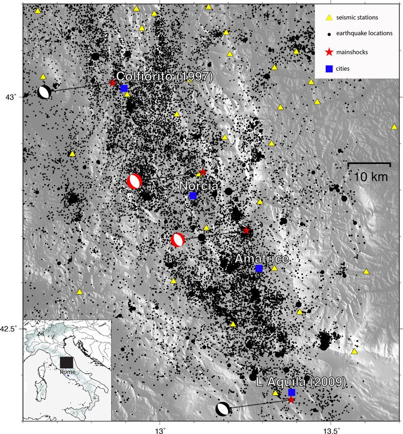
556      D. Spallarossa et al.

                                     testing of analysis techniques of seismic sequences evolution, including real-time, operational
                                     monitoring of b-value, time-dependent hazard evaluation and aftershock forecasting.
                                     Key words: Time-series analysis; Computational seismology; Seismicity and tectonics;
                                     Crustal imaging.

                                                                        seismological data from both background seismicity and periods of
1 I N T RO D U C T I O N
                                                                        enhanced activity during seismic sequences (Di Stefano et al. 2006;
On the 24 August 2016, a Mw 6.0 earthquake occurred in Cen-             Diehl et al. 2009; Satriano et al. 2011; Lomax et al. 2012; Valoroso
tral Italy near the town of Amatrice, starting a seismic sequence       et al. 2013; Spallarossa et al. 2014; Romero et al. 2016; Wollina
characterized by a cascade of moderate extensional earthquakes.         et al. 2018). They complement alternative continuous waveform-
Two months later, a Mw 5.9 earthquake occurred, on 26 October           based techniques such as template-matching (Gibbons & Ringdal
2016, near the village of Visso (Fig. 1). This activated the northern   2006; Shelly et al. 2007; Peng & Zhao 2009) and deep learning
edge of the fault system, and was followed 4 d later by the largest     approaches for earthquake phase association (Ross et al. 2018).

                                                                                                                                                  Downloaded from https://academic.oup.com/gji/article/225/1/555/6044232 by guest on 17 November 2021
earthquake in the sequence, Mw 6.5 on 30 October, near the town         All of these must guarantee an appropriate level of reliability in
of Norcia. After a further month, four moderate magnitude earth-        derived data such as phase arrival times, locations, origin times
quakes of 5.0 ≤ Mw ≤ 5.5 occurred on the 18 January 2017 near           and (local) magnitudes comparable to those obtained from man-
Campotosto, at the southern edge of the Amatrice fault system.          ual analyses, and do this for a greater number of events per unit
   The total length of the normal fault system activated by the 2016–   of computing time. Obtaining this reliability can be challenging
2017 seismic sequence is 70 km. This is a very seismically active       during seismic sequences, where events frequently overlap in time
section of the regional Central-Northern Apennines fault system,        or occur simultaneously in different parts of a network. There are
where large historical and instrumental earthquakes with Mw ≥ 6.0       three major advantages of having a larger number of events and a
have occurred in the past. These include events dated from the          smaller detection threshold in catalogues extracted from automated
13th century C.E. (Rovida et al. 2016) up to the last 30 yr, as well    processing of waveform data. The first is the better constraint on
as the 1997 Colfiorito (Chiaraluce et al. 2003) and 2009 L’Aquila       earthquake frequency–magnitude parameters used in probabilistic
(Valoroso et al. 2013) sequences. The Norcia-Amatrice sequence          seismic hazard analysis or operational earthquake forecasting from
reactivated the area in between these two earlier sequences.            the increased bandwidth of data. This increased bandwidth, and the
   The permanent RSNC network of seismic stations, operated             increased number of events, also has the potential to reduce the
by the Italian National Institute of Geophysics and Volcanology         estimated errors in such parameters. The second is the benefit from
(INGV) for the surveillance of the Italian seismic activity, has a      from introducing small magnitude events to introduce secondary
mean minimum detection magnitude of ML ≈ 0 and a completeness           triggering effects illustrated by forecast models developed for the
magnitude of ML = 1.4 in the considered period (ISIDe Working           AVN sequence (Mancini et al. 2019). Extending the inclusion of
Group 2007). Fig. 1 shows the permanent seismic network before          secondary triggering to smaller magnitudes is now possible using
the Amatrice earthquake, together with the seismic activity recorded    the high-resolution catalogue. Third, uncovering the smaller events
in the 5 yr prior to the Amatrice sequence (ISIDe Working Group         from high-resolution data may shed new light on important details
2007). Fig. 1 also shows the location and focal mechanisms of           of the fault architecture. These advantages demonstrate the im-
the earlier Colfiorito 1997 sequence to the north and the L’Aquila      portance of decreasing the threshold of detected and characterized
2009 sequence to the south (in conventional black and white in          events in improving forecasts. Gulia & Wiemer (2019) investigate
Fig. 1), and the two Mw > 6.0 events that occurred during the           whether observations of b-value variation in time can lead to alarm-
2016–2017 sequence (red/white in Fig. 1). These four events are         based forecasts but current testing of the method to other sequences
the only earthquakes with Mw > 6.0 in the last 30 yr. All the fo-       reveals some caveats for the effectiveness of potential warnings
cal solutions (TDMT—Time Domain Moment Tensor Catalogue;                (Dasher-Cousineau et al. 2020)
http://cnt.rm.ingv.it/tdmt) display clear extensional fault movement       In this work, we adopted the Complete Automatic Seismic Pro-
displayed along NW-trending normal faults, roughly parallel to the      cessor procedure (CASP; from Scafidi et al. 2019), to analyse an
strikes and dips of the mapped fault breaks.                            entire year of recordings of the 2016–2017 Central Italy seismic
   Immediately after the Amatrice main shock, the emergency team        sequence in a consistent way. We chose CASP because it proved not
of National Institute of Geophysics and Volcanology began to install    only to be fast in processing a large amount of seismological data,
22 seismic stations to complement the permanent ones. Then, sci-        but also to detect consistent P- and S-phase arrival times, allowing
entists from the British Geological Survey, with the support of the     the accurate location of events. The other techniques mentioned
NERC Geophysical Equipment Facility and SEIS-UK, deployed an            above may be able to detect more events and provide accurate rel-
additional 24 broad-band stations within the next few days, result-     ative locations, but can miss events and/or not always provide the
ing in a dense network of 155 stations, with a mean separation in the   absolute locations calculated here. The core of CASP is an advanced
epicentral area of 6–10 km. This dense seismic network produced         automatic wave arrival time detector and location software, based
over 2.5 terabytes of data in 1 yr, too much to handle by manual        on a chain of modular procedures constituted by iterative algorithms
phase picking techniques used in preparing the RefCat from RSNC         (named ‘RSNI-Picker2 ’, from: Spallarossa et al. 2014; Scafidi et al.
data by manual phase picking. Accordingly, we used automatic            2018). The pragmatic choice of CASP allows us to improve (i) de-
processing of the continuous recordings to generate a more com-         tectability, in terms of number of correctly detected arrivals times
prehensive earthquake catalogue with better locations and improved      or hit rate, (ii) reliability, in terms of minimizing the rate of false
detection of events below the previous magnitude of completeness.       or imprecise picks and (iii) accuracy of results (Scafidi et al. 2016).
Such automatic procedures have commonly been used to analyse            It also allows us to generate catalogues of events quickly (∼12 hr),
High-resolution catalogue for Central Italy (2016-17) 557
Downloaded from https://academic.oup.com/gji/article/225/1/555/6044232 by guest on 17 November 2021
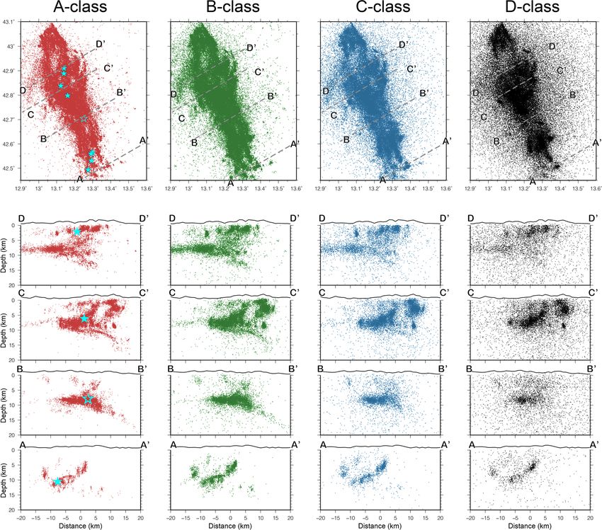
Figure 1. Map of the study area. Black circles represent earthquake epicentre locations in the 5 yr before the Amatrice Main shock (23 August 2011 to the
23 August 2016; from the Italian bulletin). The circle diameter scales with earthquake magnitude in M0.5 steps. The red stars associated with the black/white
focal mechanisms shown are the locations of the two events with Mw > 6.0 that occurred in the area in the last 30 yr (Mw 6.0 Colfiorito 1997 to the north and
Mw 6.1 L’Aquila 2009 to the south). The red stars with red/white focal mechanisms are the locations of the two events with Mw > 6.0 that occurred during the
(Central Italy) sequence studied here. Yellow triangles are the permanent seismic stations of the Italian seismic network managed by INGV.
to the point where operational earthquake forecasts could be made 2.1 The seismic network
daily. In this paper we prove this concept, and show that the new
The area affected by The Amatrice sequence had been regularly
data from the temporary stations, analysed by the CASP algorithm,
monitored before its onset by the stations of the Italian National
can reveal new features of the fault architecture and improved es-
Seismic Network (INGV Seismological Data Centre 2006) and
timates of parameters used in probabilistic seismic hazard analysis
by additional local and regional seismic networks (respectively
and operational earthquake forecasting.
the TABOO–Chiaraluce et al. 2014 and RESIICO–Marzorati et
In the Table 1, we list the properties of the RefCat and enhanced
al. 2016, networks) operated by INGV. This permanent network
catalogues. The methods used in producing the enhanced catalogue
was enhanced by the deployment of complementary set of 22 3C-
are described in more detail in the following section.
stations from the INGV emergency network of temporary, portable
stations within the first 10 d of the sequence (Moretti et al. 2016).
An additional 24 broad-band stations that were installed by the
2 P- AND S-PHASE PICKING,
10th of September, by the British Geological Survey (BGS) and
E A RT H Q UA K E D E T E C T I O N A N D
School of Geosciences at the University of Edinburgh, in active
C H A R A C T E R I Z AT I O N
co-operation with INGV to optimise the enhanced network. The
This section describes the elements of the work flow we used to final configuration of the enhanced, dense seismic network con-
retrieve the enhanced earthquake catalogue obtained by the CASP tained 155 stations (Fig. 2), bringing the station inter-distance down
method on the dense seismic network. The work flow itself is illus- to 6–10 km.
trated in the flowchart of Fig. 3.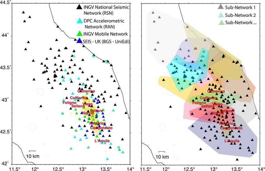
558       D. Spallarossa et al.

Table 1. Main properties of the RefCat and enhanced catalogues.
Catalogue name                                        RefCat                                                 Enhanced
Stations used                                         INGV operated permanent and temporary                  INGV/BGS/UK-SEIS enhanced network
                                                      networks
Number of station at steady state                     109                                                    155
Time window                                           24 August 2016–31 August 2017                          24 August 2016–31 August 2017
Phase picking                                         Manual                                                 Automatic
Location method                                       Hypo, Hypo2000, NonLinLoc                              NonLinLoc
Average number of phases (ML 1.4–1.5 events)          30                                                     72

                                                                                                                                                               Downloaded from https://academic.oup.com/gji/article/225/1/555/6044232 by guest on 17 November 2021
Figure 2. Final seismic network configuration (left-hand panel), colour-coded by type, and the epicentral area (coloured in yellow) and overlapping, colour-
coded, sub networks defined in the main text (right-hand panel).

Figure 3. Flow-chart of the CASP automatic procedure followed in this work.

   This network configuration operated stably from 24 August                     2.2 P- and S-phase arrival times and earthquake detection
2016 to 31 August 2017, producing a massive data set of con-
                                                                                 The CASP software analyses the recorded waveforms directly in
tinuous waveforms (≈2.5 terabytes). The data set is now freely
                                                                                 the standard miniseed format, organized in daily (24-hr) continuous
available, in standard miniseed format, from the ORFEUS (Obser-
                                                                                 time windows as retrieved by the standard seedlink archive format.
vatories & Research Facilities for European Seismology) and IRIS
                                                                                    The first step of the automatic procedure is the event detection
(Incorporated Research Institutions for Seismology) web portals
                                                                                 based on a standard STA/LTA analysis, empirically calibrated for
(https://www.orfeus-eu.org/, https://www.iris.edu/hq/).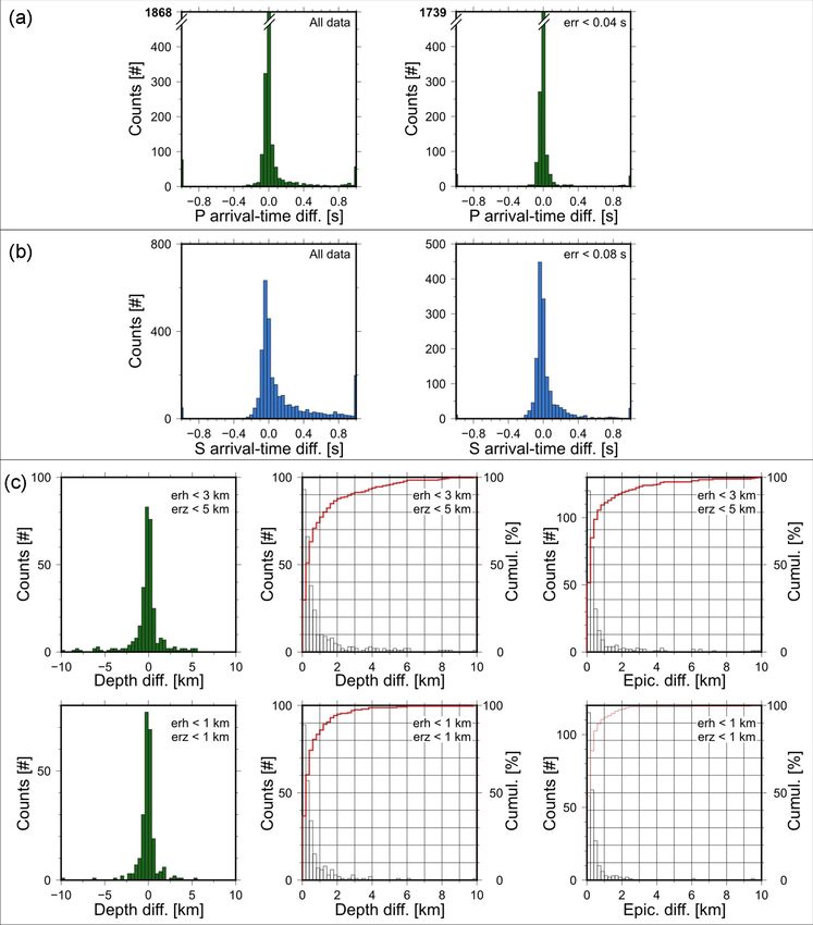
High-resolution catalogue for Central Italy (2016-17)               559

each station as a function of the site’s ambient noise and the charac-      event location, a very difficult task. The waveforms for two, or
teristics of its installed instruments. The main parameters involved        more, seismic events occurring almost at the same time could over-
in this calibration are (see Table 2): the low- and high- corner fre-       lap, leading to one or more events being missed. However, this will
quencies of the band-pass filter (F Low and F High), the short-             only occur if the signals from the most distant station for the earlier
and long-term average constants (STA and LTA), the STA/LTA ratio            event arrive around or later than those from the nearest station for
threshold (Level), the window length for the STA/LTA ratio cal-             the later event. RSNI-P2 includes a smart search component for
culation (Dur), and the minimum time-interval permitted between             such nearly contemporary earthquakes. After a first event is de-
two consecutive triggers (LenMin). These parameters have been               tected and located, the procedure dynamically cuts each waveform
set such that the algorithm is very sensitive to the occurrence of          to exclude the portions of the signal belonging to the first event.
candidate events, producing a very large number of triggers. This           This waveform cut is done by identifying the end of the seismic
minimizes the chances of failing to detect ‘true positives’, at the         signals belonging to the earlier event, and by evaluating the event
expense of also producing many ‘false positives’ associated with            magnitude (i.e. higher magnitude implies longer signals to be cut,
non-seismically generated noise. However, the false positives are           and vice versa) and the hypocentral distance from each station (i.e.
then removed on the basis of the location residuals and of the qual-        the starting time of each time window is independently selected).
ity of locations, in the final step of the CASP procedure, which has        As a consequence, the time windows available for a potential later

                                                                                                                                                      Downloaded from https://academic.oup.com/gji/article/225/1/555/6044232 by guest on 17 November 2021
been proven to discriminate effectively between true seismic phases         event are determined. Then, the system starts a new search analysis
and other signals.                                                          on these waveforms, to check for and detect any missing earthquake.
   For each trigger detected through the STA/LTA analysis, the final        A similar process is done with the part of the seismograms before
trigger time is then determined as the minimum of the Akaike In-            the first detected event, looking for other events that occurred just
formation Criterion (AIC) function (after Akaike 1974) computed             before its time window.
within a signal window around the previous trigger identification.             RSNI-P2 is also equipped with a tool for identifying out-of-
The use of the AIC-based algorithm allows us to overcome some typ-          network events such as teleseisms or regional earthquakes through
ical errors associated with STA/LTA analysis (Scafidi et al. 2019).         an appropriate spectral analysis. This algorithm is able to discrimi-
   The station trigger data were then input in into the CASP event          nate reliably between phase arrival times caused by non-local events
detection module (see Fig. 3). The detection module is based on a           in order to discard them and to have a clean final data set of local
‘coincident’ system, where a defined number of data channels must           earthquakes (Scafidi et al. 2019).
be triggered within a defined time window in order to declare the              The final results of the CASP procedure is a data set of P- and
(potential) beginning of a candidate event. It has proven to have           S-phase arrival times and an earthquake catalogue of origin time,
strong advantages in detection of events occurring close in time            location, depth and magnitude, all linked together. Every phase ar-
during a seismic sequence. Event detection was further optimized            rival time is attributed to the earthquake it belongs to, and every
by splitting the analysis into sub-networks defined by 11 different         earthquake has the list of arrival times that led to its location. This
geographical zones defined by the pattern of seismicity (Fig. 2),           provides an important benchmark for future studies based on these
allowing the accurate detection of as many events as possible. The          data. Moreover, every single result has its own error estimation,
zones overlap, but this is necessary to allow us to recognize identical     allowing the possibility to discriminate between different quality
events detected by the different networks, and hence to remove              classes. For each set of arrival times, CASP provides quality factors
duplicates in the catalogue. Accordingly, we report in Table 3, for         (qf) that indicate the estimated uncertainty of the automatic detec-
each subnetwork, the name, the number of stations included and              tion in seconds, to clearly define the reliability of each datum. The
the parameters controlling the event detection, that is the number          earthquake location quality is an output of the location software,
of stations which must be triggered within the coincidence window           specifically a probabilistic estimation of the error produced within
length.                                                                     the NonLinLoc code (Lomax et al. 2000).
   The seismograms of the potential events are then extracted from
the continuous recordings and converted in standard Seismic Anal-
ysis Code (SAC) format. Each time window has 10 s of pre-trigger
                                                                            3 F I N A L E A RT H Q UA K E C ATA L O G U E
time and a total duration of 45 s. Considering the network density,
                                                                            G E N E R AT I O N
for every triggered event we extracted waveforms from all the sta-
tions located within 90 km from the preliminary epicentre of the
                                                                            3.1 Probabilistic earthquake location with station
possible event. Then, the waveform for the candidate event is anal-
                                                                            corrections
ysed through the advanced automatic picker and location engine,
named RSNI-Picker2 (RSNI-P2 in Fig. 3; from Spallarossa et al.              The automatic analysis procedure we used in this study includes
2014; Scafidi et al. 2016, 2018).                                           an iterative location phase, designed to identify and optimize the
   The RSNI-P2 is based on an iterative procedure for the automatic         P- and/or S-arrival times. The final data set of P- and S-phase
identification of phase arrival times by calculating AIC functions.         arrival times, respectively consisting of 7016 435 P and 10 003 900
Iterations consist of different steps, separately performed for P- and      S phases. The total number of identified and associated phases with
S-phases, where arrival time identification is checked and refined          earthquakes is much greater than in RefCat. In the magnitude range
based on a preliminary earthquake location we computed with the             1.4–1.5 the average number of picked arrival times is 72 and 30
NonLinLoc software (Lomax et al. 2000) and a 1-D velocity model             for the enhanced catalogue and RefCat, respectively (see Table 1).
of the area (De Luca et al. 2009).                                          The significantly higher average number of phases of the enhanced
   Complex seismic sequences are often characterized by the oc-             catalogue with respect to the standard one is due to: the higher
currence of multiple main shocks within a short time scale going            number of stations, concentrated in the epicentral area, used for
from seconds to weeks. The likelihood of events occurring closely           the enhanced catalogue, and the iterative search procedure of S
spaced in time (even if not necessarily in space) makes the auto-           phases (see ‘P- and S-phase arrival times and earthquake detection’
matic analysis of seismic data, in terms of phase association and           paragraph).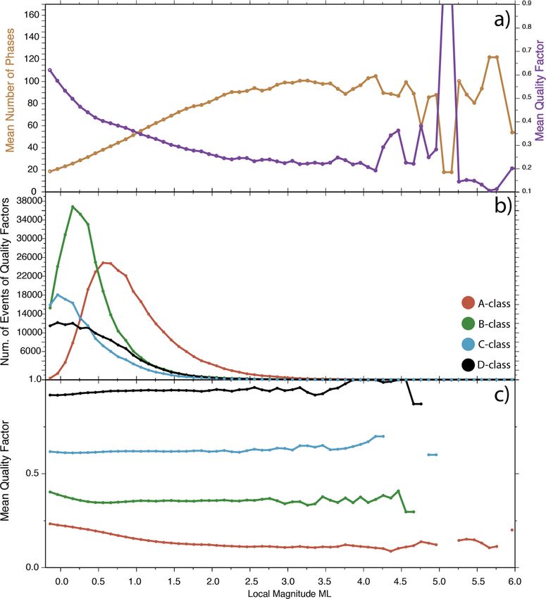
560      D. Spallarossa et al.

Table 2. Parameters involved in the STA/LTA triggering procedure.
F Low (Hz)              F High (Hz)              STA                LTA        Level             Dur (s)            PostEv (s)           LenMin (s)
10.0                        30.0                 0.8                25.0        2.0                1.5                 15.0                  60

Table 3. Subnetworks name, configuration and related parameters involved      Obviously this complete procedure of station correction would
in the STA/LTA triggering procedure.                                       not be possible in a near real-time application of the method; how-
                                                        Number of          ever a good estimate of station corrections would be available for
                   Number of       Coincidence     coincidence triggers    the permanent part of the network from background seismicity.
Subnetwork          stations       window (s)       to declare an event    Corrections for the temporary stations would be obtained with an
seq1                   45               5.0                 4
                                                                           increasing accuracy during the evolution of the sequence, but, as al-
seq2                   27               5.0                 4              ready stated, their contribution is less critical with respect to stations
seq3                   23               5.0                 4              in the Adriatic foreland, mainly permanent ones.
avts                   13               5.0                 4                 We show in Fig. 5(a) map view of the 440 697 relocated events
mrcc                   19              10.0                 4              making up the final enhanced earthquake catalogue. For compar-

                                                                                                                                                        Downloaded from https://academic.oup.com/gji/article/225/1/555/6044232 by guest on 17 November 2021
nrcn                   15              10.0                 4              ison, we also report in Fig. 6 the number of events per day of
nord                   12              10.0                 4              the obtained catalogue (in red) versus those present in the RefCat
avtn                   20               5.0                 4              (ISIDe Working Group 2007). Our procedure significantly increases
nadr                   9                5.0                 4              the number of retrieved events by a factor varying from four to more
SARD                   10               5.0                 4
                                                                           than five during the sequence, with an overall mean ratio of 5.22.
COLF                   16               5.0                 4
                                                                           This holds even during the phases of very high event rate asso-
                                                                           ciated with the major destructive events—at the beginning of the
                                                                           sequence, during the period 26–30 October 2016 and soon after the
                                                                           17 January 2017. This confirms the efficiency of the detection and
   The final data set of arrival travel times was then used as input       picking algorithms, even for seismic events that are closely spaced
to a final optimized relocation run, producing the final list of seis-     in space and time. In a recent work, Zhang et al. (2019) associate
mic events with their hypocentral location, depth, origin time and         and locate about 3300 events for a subset of 5 d of the sequence
associated uncertainties. To do this we used the same NonLinLoc            (14–18 October 2016) using the Rapid Earthquake Association and
procedure adopted for the picking phase, and the same 1-D propaga-         Location algorithm (REAL). For the same period, our automatic
tion model, derived from De Luca et al. (2009). The main difference        database includes more than 4300 well-located events.
is the introduction of static station correction values, to reduce the        After the final relocation step, we performed a final ‘cleaning’ of
discrepancies between the adopted propagation model and the real           the derived data set for P- and S-wave arrival times to remove redun-
Earth.                                                                     dant entries and to ensure consistency of outputs in the catalogue. As
   A proxy of the best station corrections can be obtained from the        a result, only those phases contributing to the final location are in-
mean residuals obtained for a set of located events. In order to reduce    cluded in the final catalogue containing the dataset of arrival times.
the trade-off between residual reduction and changes in location, a        In particular, P and S arrival times with residuals greater than 2 s or
sub-set of events with very stable locations and a redundant number        with a zero weight in the location were discarded. Nevertheless, all
of phases was selected for a benchmark test. Moreover, in order            the events contained in the final earthquake catalogue have at least
to reduce the possible impact of a non-uniform sampling of the             six P and S phases.
investigated area, events were selected by imposing a regular grid            Prior to the cleaning procedure, some 4 per cent of the loca-
(size 5 km) on the hypocentral volume of the sequence, and by              tions (18 945 events) had (unphysical) negative depths. Within those
choosing a maximum of 10 events for each grid element showing              events, there were 899 events in the A-class for quality (5 per cent),
the highest number of phases. In this way, we avoid oversampling           2888 events in the B-class (15 per cent), 4782 events in the C-class
the ray paths in the volumes with the highest number of events and         (25 per cent) and 10 376 events in the D-class (55 per cent). For
stations. Thus, a sub-set of about 3600 events was selected from the       the definition of the adopted quality classes, see Section 3.3. We
data set of preliminary locations.                                         decided to keep only the events whose depth is positive in the final
   The relevant phases were picked by in a recursive procedure, in         catalogue, that is its elevation is below the local topographic height.
which the mean station residuals of the previous location iteration        As a result, we excluded 11 871 events, 88 per cent of those in the C
were used as station correction for the following iteration. The           and D classes of poorly located events. The final dataset of arrival
cumulative root mean square of residuals tended to stabilize after         times contained entries for 6871 990 P and 9941 649 S phases.
three iterations, and the mean station residuals at this point were           The number of detected and validated P and S arrival times per
adopted as station corrections for the final location. Corrections         day for the whole analysed year is shown in Fig. 7(a). The number
were used only for stations showing a hit count larger than 50.            of S phases is always slightly higher than the P ones; this is due
A representation of the obtained station corrections is shown in           in part to the fact that the search for S phases is always driven by
Fig. 4. In general, the corrections in the epicentral area defined by      a trial location that is already reliably known from the P-phases.
the cloud of seismicity in Fig. 1 are rather small, confirming the         In addition, mainly for small events, very often the signal to noise
validity of the adopted 1-D velocity model. Conversely, stations in        ratio of S waves (with respect to P coda) on horizontal components
the Adriatic foreland (on the eastern side of the area studied), show      is higher than the SNR of P waves (with respect to pre-event noise)
systematically positive station corrections. This is consistent with       on the vertical component. A typical example is reported in Fig. 8,
relatively low velocities being present at the surface and in the upper    (two stations of event 170 315 000 204, Ml 0.17). Station ED19 has
crustal layers in this area, as proposed independently by Carannante       a good P- and S-picking. For the temporary station T1256, automatic
et al. (2013) in their tomographic study.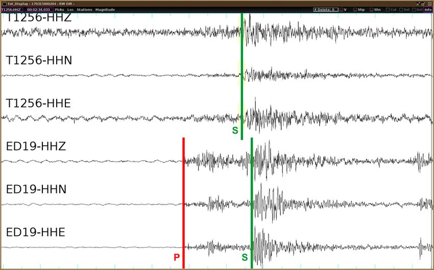
High-resolution catalogue for Central Italy (2016-17)                        561

                                                                                                                                                                        Downloaded from https://academic.oup.com/gji/article/225/1/555/6044232 by guest on 17 November 2021
Figure 4. Representation of the static stations corrections for P (left-hand panel) and S waves (right-hand panel) as colour coded circles (grey and white for
negative/positive corrections, respectively), containing the station name and the correction value (in seconds); the circle size is scaled with the correction value.

                                                                                      phases is also reported in Figs 7(b) and (c). The average value of
                                                                                      the estimated errors in the arrival times is ±0.05 s for the P phases
                                                                                      and ±0.13 s for the S phases. More than 90 per cent of arrival times
                                                                                      had estimated errors below 0.1 and 0.25 s, respectively, for the P
                                                                                      and S waves.

                                                                                      3.2 Validation of results
                                                                                      In order to evaluate the effectiveness and accuracy of the automated
                                                                                      phase picking algorithm, we analysed a subset of the data where
                                                                                      we were confident in the phase data obtained by manual phase
                                                                                      picking methods. We chose a day with a number of events close
                                                                                      to the long-term average and without any particular clustering, so
                                                                                      that the space, time and magnitude distribution of this subset can be
                                                                                      assumed to be representative of the whole data set. We selected the
                                                                                      7 January from 00:00 UTC to 06:00 UTC and hand-picked phases
                                                                                      for all the events recognized by the detection procedure, resulting in
                                                                                      345 events with both a good quality location based on the manual
                                                                                      picks, and a corresponding event in the automatic data set. It was
                                                                                      then straightforward to compare the phase and catalogue parameters
                                                                                      for these two independently generated data sets.
                                                                                         We compare the automatic and manual picks and locations (epi-
                                                                                      centre and depth) in Fig. 9. Fig. 9(a) shows the time differences
Figure 5. Map view of the seismicity distribution comprising all the 440 697
                                                                                      for the P phase picks: on the left the whole data set is analysed,
events retrieved by this study by analysing 1 yr of recorded data, with focal
mechanisms as indicated. Colour coding is the same as for Fig. 1.                     while on the right only the best quality picks are plotted. It is quite
                                                                                      evident that for P phases most picks are either nearly coincident
                                                                                      with the human ones or, in few cases, completely wrong (errors
P-picking was not possible due to the low SNR, nevertheless the S                     larger than 1s are all reported in the last bin). Fortunately, these
arrival was correctly recognized.                                                     large errors are recognized as outliers by the location procedure
   In the most seismically active single day, on the end of October                   without any further tuning, and hence are not used for the final
2016, more than 75 000 P arrival times and 110 000 S arrival times                    comparison.
were detected and correctly assigned to more than 3500 events. The                       After removing these events, the distributions of differences in
distribution of the automatic quality estimation of both P and S                      arrival time, epicentral location, and depth are even more peaked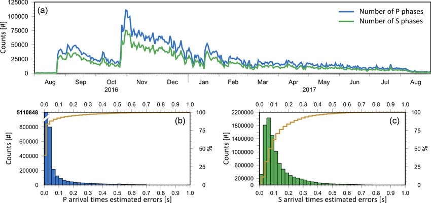
562       D. Spallarossa et al.

                                                                                                                                                                     Downloaded from https://academic.oup.com/gji/article/225/1/555/6044232 by guest on 17 November 2021
Figure 6. Number of events per day in the enhanced catalogue (black) versus RefCat catalogue (red).

Figure 7. (a) Number of P (blue) and S (green) arrival times per day; (b and c) incremental distribution of P- and S-arrival times estimated errors, respectively,
with cumulative probabilities in yellow.

(and the number of large errors reduced). The estimated system-                     the phase arrival time, and to discriminate reliable results from
atic error in the automated phase picks estimated by the difference                 outliers.
between the high-confidence manual and automated picks is less                         The locations obtained by the automatic picks in the test period
than 0.04 s: the level of confidence is 87.0 per cent within this                   were then compared with those of the representative sample of the
threshold, and 93.3 per cent within 0.08 s. For S picks, the dis-                   manual ones. Fig. 9(c) in the top row shows histograms of the depth
tribution appears broader (Fig. 9b, left-hand panel), and is again                  difference (automatic minus manual depth), the modulus of differ-
skewed towards positive values, implying delayed picking in the                     ence in depth distance, and the modulus of difference in epicentral
automatic system. If we reduce the analysis to the best quality picks               for events with estimated horizontal errors below 3 km and verti-
(estimated errors below 0.08 s, Fig. 9b, right-hand panel) the distri-              cal errors below 5 km. Some 94.1 per cent of the locations show
bution appears narrower and more symmetric. In this case, 72.6 per                  horizontal distances below the threshold of 3 km, and 95.5 per cent
cent of the differences are below the threshold, and 85.2 per cent                  below the 5 km threshold for the depth error. The depth difference
below twice this value. For both P and S picks the distribution of                  appears nearly symmetrical, showing that the automatic procedure
the systematic error is somewhat asymmetric, with a slight skew                     does not introduce any systematic bias in the depth estimate.
to positive values, implying the automatic pick is slightly biased                     If we reduce the analysis to the more reliable locations (horizontal
to be later than the human one. These results confirm that the S                    and vertical error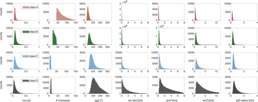
High-resolution catalogue for Central Italy (2016-17)                   563

                                                                                                                                                              Downloaded from https://academic.oup.com/gji/article/225/1/555/6044232 by guest on 17 November 2021
Figure 8. Example of automatic P and S phase picking for two stations. For the temporary station T1256, automatic P-picking was not possible due to the low
SNR, nevertheless the S arrival was correctly recognized.

section, these results provides a firm validation of the accuracy of             would be the lowest. In turn, this is consistent with a lower-mean
the phase picking method in comparison with manual analysis of                   number of phases contributing to the earthquake locations for the
the same data for a representative sample of data.                               low-quality data. The quality factor is quite constant for different
                                                                                 earthquake magnitudes for all quality classes (Fig. 11e). 4.0. Fi-
                                                                                 nally, for the higher values of magnitude, we observe a degree of
3.3 Quality of earthquake locations                                              volatility in the mean qf and in the number of phases (see Fig. 11c).
                                                                                 We know that the automatic picks for (the usually small number
In order to classify the quality of the final earthquake locations,
                                                                                 of) moderate-to-large earthquakes that occur during one seismic
we applied the procedure proposed by Michele et al. (2019) to the
                                                                                 sequence strongly depend on factors not considered here, for ex-
resulting catalogue. These authors proposed a criterion to assess the
                                                                                 ample instrument clipping or the presence of a minor event within
location quality, consisting of the combination of the uncertainty
                                                                                 the nucleation phase. Thus it may be advisable even with an au-
estimates, properly normalized, provided by the NonLinLoc loca-
                                                                                 tomated phase picking method to continue to analyse data for the
tion code (Lomax et al. 2000). The procedure quantifies the location
                                                                                 relatively few largest events manually for the time being, at least
quality estimate in terms of a unique numeric normalized value the
                                                                                 until automated techniques have been adapted to account for such
quality factor which varies between qf = 0 (best quality location)
                                                                                 effects.
and qf = 1 (worst quality location). Then, the location obtained
is assigned to a quality class depending on the qf parameter value
according to the following scheme: A-class (0 < qf ≤ 0.25), B-
                                                                                 3.4 Local magnitude (ML ) computation
class (0.25 < qf ≤ 0.50), C-class (0.50 < qf ≤ 0.75) and D-class
(0.75 < qf < 1.00). We report in Fig. 10 the distribution of the loca-           The local magnitude (ML ; Richter 1935, 1958) is also calculated
tion parameters, divided into these different quality classes (class:            automatically, using the complex multithread algorithm embed-
A in red, B in green, C in blue and D in black). The parameter distri-           ded inside RSNI-P2. Since ML could be strongly biased by the
butions all show increasing dispersion while moving from the best                signal processing methods adopted to correct for instrument re-
(A) to the worst (D) class, with the single exception of the plots for           sponse, we also adopted an automatic method to select the best
the number of phases picked, where the distribution narrows with                 pre-deconvolution filter parameters on the basis of signal-to-noise
decreasing quality, and the average number of phases identified also             analysis. Specifically, the high-pass corner frequency of the Butter-
decreases. These results are not inconsistent with each other—we                 worth pre-deconvolution filter is automatically determined, identi-
would expect better locations and a more variable number of phase                fying the lowest frequency (in the 0.5–2.0 Hz range), which gives a
picks in good quality data. We end up with a catalogue of earth-                 signal-to-noise ratio greater than a threshold value (e.g. usually 4.0).
quake locations, distributed between the quality classes as A-31.8               This approach allows the proper consideration of the relatively low
per cent, B-32.0 per cent, C-18.3 per cent and D-17.9 per cent. The              frequencies, around 0.5 Hz, relevant for earthquakes with higher
relationship between the main location parameters as function of                 magnitudes (e.g. ML > 3). This is important to avoid ML underes-
the magnitude is shown in Fig. 11. The reported quality factors qf               timation for these events. On the other hand, the lower frequencies
are mean values computed in bins of 0.02 of magnitude. The mean                  are discarded in the case of low-magnitude earthquakes recorded
quality factor and the number of phases picked is fairly constant in             by broad-band instruments in order to minimize any bias from
the magnitude range 2.0–3.6 (see Figs 11a and b). Each class has                 microseismic noise. The low-pass corner frequency of the Butter-
a quality factor that is peaked around a magnitude that increases                worth pre-deconvolution filter is always selected on the basis of the
systematically with increasing quality. This is consistent also with             sampling frequency such that it is always lower than the Nyquist
the distribution of the number of events in Fig. 11d), where the                 frequency.
higher quality data peaks at a higher magnitude, and the lower qual-                After an earthquake is located and seismic signals are filtered
ity data peaks at low magnitudes where the signal to noise ratio                 with the above procedure, ML is automatically evaluated using the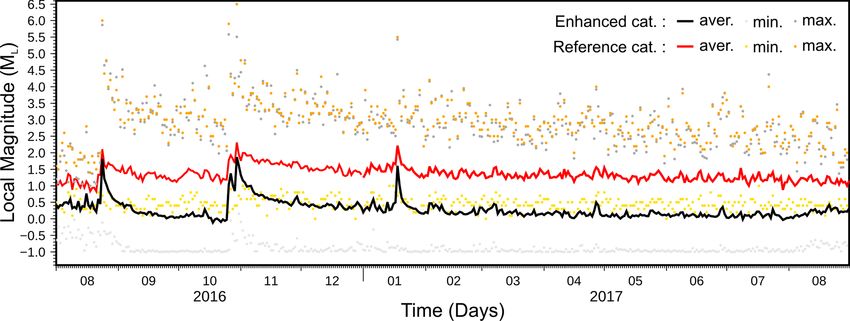
564      D. Spallarossa et al.

                                                                                                                                                          Downloaded from https://academic.oup.com/gji/article/225/1/555/6044232 by guest on 17 November 2021
Figure 9. Comparison between automatic and manual picks and locations for the selected representative sample of events. (a) Comparison of P picks times
(automatic—manual). Left-hand panel: whole data set; right-hand panel: estimated picking error
High-resolution catalogue for Central Italy (2016-17) 565
Downloaded from https://academic.oup.com/gji/article/225/1/555/6044232 by guest on 17 November 2021
Figure 10. Statistical distribution of the location parameters used as input to evaluate the location quality factor.
Figure 11. (a) Mean number of phases (brown) and mean quality factor (purple) as a function of magnitude. (b) Mean number of events versus magnitude,
divided by quality classes. (c) Mean quality factor (qf) versus magnitude, divided by quality classes.
epicentre. Finally, if the number of remaining data values after the is recomputed also excluding the minimum and maximum single
previous selections is greater than a given threshold (e.g. 6), ML566 D. Spallarossa et al.
station magnitude values to reduce the influence of potential out- extracted category D low-quality events (qf > 0.75) falling in cells
liers. Otherwise, the initially computed ML value remains valid. All with a minimum distance of 5 km from each cell populated by events
of these steps are automated, reproducible and consistently applied from the A + B catalogue. These events are the most likely to have
once the control parameters have been chosen. poor locations and hence are the most likely to be associated with a
potentially artificial seismic ‘cloud’. We obtain 327 events with this
criterion, 0.07 per cent of the whole catalogue. This means that the
wide cloud of seismicity recognizable in maps and cross-sections
4 R E S U LT S
(Fig. 12) of D-quality events is generated by rather few poorly-
Fig. 12 shows the spatial distribution of all the events contained located events. Moreover, if we compute the mean quality factor of
in the enhanced earthquake catalogue obtained by the methods de- this sub-set of events, we obtain a value of 0.97 (qf ranges from 0 for
scribed in section 2. The plot is divided into four columns, one for the best location to 1 for the more unstable ones). It is evident that
each location class based on the quality factor (qf) defined above this sub-set of events belongs to the tail of our error distribution, and
(from class A to class B, C and D). The cross sections are drawn do not add to our understanding of fault architecture or potential
across the largest events of the sequence. Section A crosses the south seismic zoning in the region.
the cluster of four Mw > 5 events of January 18, sections B and C To investigate what these locations represent in more detail, we vi-
Downloaded from https://academic.oup.com/gji/article/225/1/555/6044232 by guest on 17 November 2021
cut through the Mw 6.0 Amatrice and Mw 6.5 Norcia main shock, sually inspected some of their waveforms. We found a few examples
respectively, and the northernmost section D crosses the location of of real earthquakes located far from the sequence source area (the
the Mw 5.9 Visso earthquake. true sparse background seismicity), but mainly the cloud is com-
The enhanced catalogue consists of 440 697 events, with— prised of mislocated events, often linked to nearly-contemporaneous
1.0 ≤ ML ≤ 5.9, and covers the first year of the Central Italy seismic events not correctly managed by the automatic picking procedure.
sequence, starting from the 24 August 2016 (the date of the first Am- The cloud is therefore an artefact of poorly located events. This
atrice main shock) to the 31 August 2017 (the date of the removal quality check confirms that the quality factor is a good discriminant
of the BGS temporary seismic stations). for the reliability of the location. For applications related to the
Despite the differences in quality, the general pattern of the seis- reconstruction of structure geometries we would thus recommend
micity in the different classes is remarkably consistent in both hor- using only the best-quality events (low qf) while for a purely sta-
izontal and vertical projections (Fig. 12). The locations for the two tistical analysis (i.e. b-value analysis), when a mislocation of some
best quality classes (A and B), are absolutely comparable to those km could be not critical, the whole catalogue may be used.
based on manual phase picks by Michele et al. (2016), Chiaraluce The enhanced seismicity catalogue provided by the CASP proce-
et al. (2017) and Improta et al. (2019). The general pattern is also dure provides a much clearer picture of the activated structures than
clearly resolved by the lower quality data (C and D) at the kilometre before. For example, we observe 1) new geological structures, for
scale of the diagram. example a fault located in the footwall of the system in section C
In order to quantify the clustering characteristics of the RefCat not detected in the previous work and 2) shallow (< 5 km of) depth
and of the new catalogue, we subdivided the whole volume inter- earthquakes that partly fill portions of the shallower crustal vol-
ested by the sequence in 242 000 cubic cells with 1 km long edges, ume previously characterized by low seismic activity (e.g. sections
and counted the events falling in each cell. For the RefCat, 83 326 B along the Amatrice fault plane (cf. Michele et al. 2016, 2020;
events fell in the selected volume and they occupied 12 950 cells Chiaraluce et al. 2017; Improta et al. 2019).
(5.3 per cent of the total); 90 per cent of the earthquakes used just All the main events with Mw > 5.0 are well located by the CASP
6201 cells (2.6 per cent of the total). If we select just the A-class algorithm, with the single exception of the first Amatrice main shock
events (qf < 0.25) of our new catalogue, we obtain 140 122 events (Mw = 6.0) which has an estimated depth of 0 km. This was most
in the selected volume and they use 11 369 cells (4.7 per cent); 90 likely a consequence of (i) a lower number of stations (at this stage
per cent of the events is limited in 4328 cells (1.8 per cent). In just the permanent ones were available) and (ii) the low number of
conclusion, even taking into account just the best quality locations, strong motion sensors with non-clipped data. In combination, these
we obtain a higher number of events in a source volume more re- resulted in a non-optimal location, so we excluded it from the final
duced with respect to those of the RefCat. If we also include the catalogue.
B-class events (quality factor < 0.50), we obtain 281 017 events, Our results clearly demonstrate the high performance and ro-
using 18 671 cells (7.7 per cent); 90 per cent of these are limited to bustness of the automatic CASP procedure (Scafidi et al. 2019) in
5717 cells (2.4 per cent). This selection reports a number of events retrieving a large number of well-constrained events, along with
3.37 times higher than the RefCat and still with a higher clustering better estimates of their location, and a more complete catalogue at
factor. It must be remembered that the RefCat is based on manual low magnitude. To illustrate the improvement in completeness, the
phase pickings, while the high resolution catalogue is fully auto- frequency–magnitude distributions for the RefCat and for the en-
matic. If we analyze the whole new catalogue (434 596 events in hanced catalogue are shown in Fig. 13. The estimated completeness
the volume), we fill 39 223 cells (16.2 per cent), but the majority magnitude for the enhanced catalogue is close to ML 0.6, indicated
(90 per cent) are in 10 839 of these (4.5 per cent). As expected, and by the upper end of the red line, is almost one magnitude unit better
as evident in the maps and in the cross-sections, the lower quality than that of the RefCat catalogue (ML 1.4 indicated by the upper
events are more dispersed forming a diffuse cloud around the whole end of the blue line). The b and a value (see Fig. 13) of the G-R
area. Nevertheless, even for the whole catalogue the majority of the relationships and their respective uncertainties are computed using
events are concentrated in a limited volume, indicating significant a maximum-likelihood assessment. The b value for the enhanced
localization of seismicity—well located small events do not stray catalogue is 0.965 and for the RefCat is 1.110. The significant dif-
too far from the volumes affected by larger ones. ference in the b value and in the cumulative number of events in
The quantitative contribution of this dispersed seismicity to our the magnitude range 1.4–2.4, apparently complete for both cata-
knowledge of the process is a matter for debate, mainly due to logues, in our opinion is related to an overestimation of ML induced
the low quality of their locations. To investigate their effect, weHigh-resolution catalogue for Central Italy (2016-17) 567
Downloaded from https://academic.oup.com/gji/article/225/1/555/6044232 by guest on 17 November 2021
Figure 12. Maps and cross-sections of the events divided by the classes defined in section 3.3.
by the procedure used in the routine INGV analysis for the Ref- detected events. Most of this computation time is spent by the Non-
CAT catalogue, particularly for low-magnitude events. Indeed the LinLoc location procedure because several iterations of picking and
adoption, in the CASP method, of a high-pass filter adapted to the location for both P and S phases are required to achieve a stable
signal-to-noise ratio allows to reduce the possible bias on magni- and reliable result. The 12-hr computational time is critical since
tude estimates of the microseismic noise recorded by broad-band it will allow effectively real time catalogues to be produced, even
sensors and superimposed to the earthquake signal. for operational aftershocks forecasts updated daily during a large
seismic sequence. The improvement in magnitude of completeness
threshold of the automatic procedure will benefit the current Op-
5 DISCUSSION erational Earthquake Forecast scheme in Italy (Marzocchi et al.
High-resolution earthquake catalogues will allow us to improve fu- 2014) since the predictive power of short-term clustering models
ture operational earthquake forecasting by extending the retrospec- is directly related with the inclusion of small magnitude events en-
tive experiments where the focus is to improve our understanding hancing secondary earthquake-to-earthquake triggering. We expect
for earthquake triggering mechanisms. One of our main motiva- that the benefits from such catalogues will extend to retrospective
tions was to prove the concept that CASP would allow us to provide efforts investigating the temporal evolution of earthquake sequences
high-resolution earthquake catalogues in near-real time. In prac- through the estimation of statistical parameters, such as the b-value
tice, CASP is able to detect and locate more than 2.8 events per of the frequency-magnitude distribution that has been extensively
minute and took less than 12 hr of computation time on a stan- used in a variety of seismotectonic environments to predict haz-
dard workstation equipped with an Intel Core i7–7700 CPU using ardous behaviour through b-value decreases (e.g. Tormann et al.
4 parallel threads to analyse 1 d of data containing more than 3000568 D. Spallarossa et al.
network stations have been deployed at the start of the time period
shown, and then increases again to 0.6 when the stations are re-
moved towards the end of the time window. This improvement in
quality with respect to the number of stations is not a surprise, but
Fig. 15 confirms how the impact is significant in this case.
CASP is only one of the innovative techniques currently able to
provide very large earthquake catalogues. Template-matching ap-
proaches (TM; Shelly et al. 2007; Peng & Zhao 2009 among others)
for example, exploit the similarity of earthquake waveforms be-
tween closely-spaced events, allowing the detection of earthquakes
previously hidden in the noise. This approach has successfully been
applied in a number of examples, including induced seismicity en-
vironments (Skoumal et al. 2015). A major disadvantage is that
the method is insensitive to event templates that are absent from
the starting catalogue, such as events occurring in volumes that
Downloaded from https://academic.oup.com/gji/article/225/1/555/6044232 by guest on 17 November 2021
were previously inactive. Template matching of itself does not pro-
duce absolute P- and S-arrival times, and hence does not allow the
absolute location of all the newly detected events. Instead, such cat-
alogues often quote relative locations associated with phase shifts
identified in the cross-correlation procedure. As a consequence,
Figure 13. Frequency magnitude distributions for the enhanced catalogue
while it is usually possible to improve the number of detected events
(red) and RefCat (green). The b and a values and their respective uncertain-
ties are computed using a maximum-likelihood assessment
by more than a factor of 10, the number of well-located events typ-
ically increases only by a factor of 2–5 (Diehl et al. 2017 and Ross
et al. 2019), compared to a factor 4–5 here with the CASP procedure
2015 for tracking post-2011 seismicity in Japan). The lower magni- (Fig. 6).
tude of completeness is one of the major advantage of the enhanced More recently, profiting of the dramatic progress made by neural
catalogue, because it provides a broader bandwidth of observations networks in deep machine learning, new approaches have been
with which to test the hypothesis of a scale-invariant (power-law) proposed for both phase detection and picking (Ross et al. 2019; Zhu
distribution of source rupture area, seismic moment or energy in- & Beroza 2019). At the cost of a non-trivial training stage, needed
ferred from the magnitudes. The broader bandwidth of observations to teach the system how to recognize body waves arrival times,
in principle also reduces the uncertainty in a and b (e.g. Main 1996), the major benefit is to extract a very large number of probability
both critical parameters in both probabilistic seismic hazard analy- distributions for the presence of a P wave, S wave and noise in
sis (where they are assumed stationary) and operational earthquake continuous waveform data. By applying a series of filtering and
forecasting (where they may change with time). However, the re- decimation operations, these features are automatically extracted
sults presented here indicate there are some outstanding issues to and classified. These new systems seem to be able to work properly
address in terms of systematic effects magnitude determination and on relatively new data, whose characteristics may differ from those
scaling before this potential can be realized. in the training set. Once the seismic phases have been detected,
Despite these results, there is still some work to do in order to there is still the need to generate phase association, a challenging
increase the resolution power during the busiest time windows (e.g. task given the amount of data collected at a large number of closely
hours-days) of aftershock activity associated with the occurrence spaced stations during a seismic sequence, and often requiring tuned
of the largest events. As shown in Fig. 14, the mean magnitude of with user-defined parameters.
the events within the CASP catalogue, increases from a background Our approach is able to detect P- and S waves absolute arrival
value around ML 0.5 up to ML 2.5 soon after the occurrence of all times, allowing the accurate location and magnitude computation
of the Mw > 5 events (indicated by the black vertical lines). This is for hundreds of thousands of both very small events (down to neg-
particularly evident around the end of October 2016 when two large ative magnitudes) and events occurring in areas and fault portions
events occur within a short interval time, that is the Visso 26th and previously silent. A first-order comparison of our catalogue with
Norcia 30th of October shocks. These early aftershock phases are those generated by both template matching and deep learning ap-
the only times when the detection capability of the CASP method proaches, demonstrates that our approach performs well, at least
becomes almost comparable to that of the Italian seismic monitoring in terms of detection rate. Our catalogue covers a small area of
room. about 7000 km2 for 1 yr of seismic activity, and we compare its
We have highlighted several important outcomes achieved by us- performance to that of the QTM catalogue (Ross et al. 2019), cov-
ing the CASP procedure. Nevertheless, it is also worth remembering ering 10 yr (2008–2017) of seismic activity for Southern California
that one of the key controls on resolution is the availability of a large generated by the template matching approach. Ross et al. (2018)
number of densely spaced 3-component seismic stations. To exem- identified about 495 earthquakes per day across the region with an
plify this, Fig. 15 shows the evolution of the mean quality factor qf average time of 174 s between events. Our mean detection rate is
for the hypocentre locations defined in Section 3.3, as a function of about 1230 per day, with an average time between events of 70 s.
the number of available stations. The number of available stations During periods of intense seismicity, with peaks of more than 3000
ramps up while the temporary network was under installation in events per day, the average inter-event time is about 30 s (Fig. 6).
the early days of the sequence, while it winds down when they are These values are comparable to those obtained by Ross et al. (2019)
removed towards the end. Overall, there is a clear inverse correla- using their deep learning approach for the first 12 hr of the 2016
tion between the number of stations used in the location and qf. For Bombay Beach sequence; resulting in about 1000 events in 12 hr
example, qf decreases from around 0.65–0.45 when the temporary and an average time between events of about 40 s. In future work,You can also read