Bedrock river erosion through dipping layered rocks: quantifying erodibility through kinematic wave speed - Earth ...
←
→
Page content transcription
If your browser does not render page correctly, please read the page content below
Earth Surf. Dynam., 9, 723–753, 2021
https://doi.org/10.5194/esurf-9-723-2021
© Author(s) 2021. This work is distributed under
the Creative Commons Attribution 4.0 License.

           Bedrock river erosion through dipping layered rocks:
           quantifying erodibility through kinematic wave speed
                                             Nate A. Mitchell and Brian J. Yanites
               Department of Earth and Atmospheric Sciences, Indiana University, Bloomington, Indiana, USA
                                 Correspondence: Nate A. Mitchell (natemitc@indiana.edu)

                                  Received: 29 January 2021 – Discussion started: 24 February 2021
                              Revised: 27 May 2021 – Accepted: 14 June 2021 – Published: 21 July 2021

       Abstract. Landscape morphology reflects drivers such as tectonics and climate but is also modulated by under-
       lying rock properties. While geomorphologists may attempt to quantify the influence of rock strength through
       direct comparisons of landscape morphology and rock strength metrics, recent work has shown that the con-
       tact migration resulting from the presence of mixed lithologies may hinder such an approach. Indeed, this work
       counterintuitively suggests that channel slopes within weaker units can sometimes be higher than channel slopes
       within stronger units. Here, we expand upon previous work with 1-D stream power numerical models in which
       we have created a system for quantifying contact migration over time. Although previous studies have devel-
       oped theories for bedrock rivers incising through layered stratigraphy, we can now scrutinize these theories with
       contact migration rates measured in our models. Our results show that previously developed theory is generally
       robust and that contact migration rates reflect the pattern of kinematic wave speed across the profile. Further-
       more, we have developed and tested a new approach for estimating kinematic wave speeds. This approach utilizes
       channel steepness, a known base-level fall rate, and contact dips. Importantly, we demonstrate how this new ap-
       proach can be combined with previous work to estimate erodibility values. We demonstrate this approach by
       accurately estimating the erodibility values used in our numerical models. After this demonstration, we use our
       approach to estimate erodibility values for a stream near Hanksville, UT. Because we show in our numerical
       models that one can estimate the erodibility of the unit with lower steepness, the erodibilities we estimate for
       this stream in Utah are likely representative of mudstone and/or siltstone. The methods we have developed can
       be applied to streams with temporally constant base-level fall, opening new avenues of research within the field
       of geomorphology.

1   Introduction                                                    Miller et al., 2013; Yanites et al., 2017), and (4) searching for
                                                                    spatial patterns in rock strength (Allen et al., 2013; Bursztyn
Geomorphologists seek to extract geologic and climatic in-          et al., 2015). This last application is our focus here; to what
formation from landscape morphology, and the conceptual             extent can river morphology be used to detect spatial patterns
framework of the stream power model (Howard and Kerby,              in rock strength? While such a question seems straightfor-
1983; Whipple and Tucker, 1999) has driven many such en-            ward to address (e.g., comparing morphologies in different
deavors (Whipple et al., 2013). Indeed, as a representation         rock types), the mere presence of different rock strengths in-
of bedrock river incision, the stream power model has been          troduces complicating factors. For example, contact migra-
used in many applications, including (1) identifying unrec-         tion perturbs the spatial distribution of erosion rates, causing
ognized earthquake risks (Kirby et al., 2003), (2) constrain-       dramatic variations in slope along a bedrock river (Forte et
ing the timing and extent of normal fault activity (Whittaker       al., 2016; Perne et al., 2017; Darling et al., 2020). Surpris-
et al., 2008; Boulton and Whittaker, 2009; Gallen and Weg-          ingly, these perturbations can even cause streams to counter-
mann, 2017), (3) distinguishing between potential drivers of        intuitively have steeper reaches in weaker rocks (Perne et al.,
transient incision (Carretier et al., 2006; Gallen et al., 2013;

Published by Copernicus Publications on behalf of the European Geosciences Union.
724                                      N. A. Mitchell and B. J. Yanites: Bedrock river erosion through dipping layered rocks

2017). Predicting how contrasts in rock strength are reflected      strength would be hindered by uncertainties regarding varia-
in topography, and specifically river profiles, is therefore nec-   tions in erosion rate. To improve our capacity to extract rock
essary to advance our understanding of both (1) the drivers of      strength information from topography, we must understand
landscape evolution and (2) how we can use landscape mor-           the influence of such complications.
phology to extract information about geology and climate.              Figure 2 shows several conceptual models for bedrock
                                                                    river incision through layered stratigraphy. We have based
1.1   Motivations
                                                                    these conceptual models on previous work (Perne et al.,
                                                                    2017; Darling et al., 2020) and present them to help guide the
Forte et al. (2016) demonstrated how rock strength perturba-        reader’s understanding of this study’s focus. Clearly, more
tions can cause long-lasting landscape transience, even with        complicated situations are likely in nature (e.g., a multitude
constant tectonic and climatic forcing. The spatiotemporal          of lithologies with variable thicknesses, contact dips that vary
distribution of erosion rates can strongly vary with rock type,     over space), but our intention here is to present simple ex-
with one rock type eroding well above the rock-uplift rate          amples. In Fig. 2a, we show the river reaches underlain by
and another well below it. These findings have far-reaching         rock type 2 to be steeper than those underlain by rock type 1.
implications for landscape evolution and methodological ap-         Conventionally, this contrast would lead geomorphologists
proaches to quantifying rates. For example, the exposure of a       to suspect that rock type 2 has a higher resistance to erosion
new lithology could trigger an increase in erosion rates, and       than rock type 1. As we discussed above, however, reaches in
this increase could be mistakenly attributed to a change in ex-     rock type 2 may be steeper because they have higher erosion
ternal forcing such as climate. Variations in erosion rate due      rates (Perne et al., 2017). Note that such variations in steep-
to mixed rock types can influence detrital zircon geochronol-       ness due to rock strength contrasts could be misinterpreted
ogy, detrital thermochronology, and detrital cosmogenic nu-         as having a different driver (e.g., changes in base-level fall
clide analysis (Carretier et al., 2015; Forte et al., 2016; Dar-    rates). Figure 2b shows the stream in Fig. 2a at a later time;
ling et al., 2020). Spatial contrasts in rock strength can also     the balance between ongoing uplift (or base-level fall) and
influence detrital geochronology (Lavarini et al., 2018), so        river incision causes the contacts to gradually migrate up-
spatial variations in both rock strength and erosion rate would     stream along the stream profile. In Fig. 2c, the units dip in
further complicate the interpretation of grain age distribu-        the upstream direction (i.e., a negative contact dip). In this
tions. Furthermore, the presence of a dipping contact separat-      case, the contacts will continue to migrate upstream but the
ing lithologies with different strengths can significantly influ-   magnitude of channel slope relative to contact slope varies
ence knickpoint migration following changes in rock-uplift          along the profile. As a result, the influence of contact migra-
rates (Wolpert and Forte, 2021), highlighting the influence of      tion on erosion rates will vary along the profile (Darling et
rock properties on the transient adjustment of landscapes.          al., 2020). This consequence also applies to the river in Fig.
   As an illustrative example, Fig. 1a shows an area where          2d, which is underlain by units dipping in the downstream di-
rivers flow over layered stratigraphy near Hanksville, UT.          rection (i.e., a positive contact dip). Interestingly, when units
The streams are underlain by highly variable sedimentary            dip in the downstream direction the contacts can migrate up-
units gently dipping to the west. As the channels flow over         stream or downstream. The direction of contact migration
these different units, they exhibit pronounced changes in           depends on the contrast between channel slope and contact
channel steepness (ksn , slope normalized for drainage area;        slope (Darling et al., 2020). Importantly, in each conceptual
Wobus et al., 2006). Indeed, these changes are so dra-              model shown in Fig. 2 the spatial distributions of erosion
matic that the profiles have an unusual “stepped” appearance        rate, steepness, and contact migration rate all depend on inci-
(Fig. 1b and c). A logical approach to exploring how these          sion model parameters such as erodibility (Perne et al., 2017;
morphologies reflect rock properties would involve (1) quan-        Darling et al., 2020). By understanding these landscapes, we
tifying variations in steepness from digital elevation mod-         may be able to capitalize on these effects and quantify erodi-
els (DEMs), (2) collecting metrics of rock strength in the          bility in new ways.
field, such as Schmidt hammer measurements (Murphy et
al., 2016) or fracture density (Bursztyn et al., 2015; DiBi-        1.2   Research approach
ase et al., 2018), (3) measuring the compressive and/or ten-
sile strengths of rock samples taken in the field (Bursztyn et      In this contribution, we focus on how to use contact migra-
al., 2015), and, finally, (4) exploring patterns between chan-      tion to gain insight into bedrock river behavior and quantify
nel steepness and metrics of rock strength (Bernard et al.,         erodibility. Rather than being a complication to be avoided,
2019; Zondervan et al., 2020). Indeed, the erosion of bedrock       the perturbation introduced by contact migration can be ex-
rivers through this stratigraphy presents a seemingly conve-        ploited for model calibration in a manner similar to how
nient opportunity to explore the influence of rock strength.        one would exploit a transient response to tectonics (Whip-
If, however, the migration of contacts along these streams          ple, 2004). Although previous work has developed theories
has perturbed the spatial distribution of erosion rates, then       for bedrock river incision through layered rocks (Perne et al.,
identifying relationships between channel steepness and rock        2017; Darling et al., 2020), these theories have not been thor-

Earth Surf. Dynam., 9, 723–753, 2021                                                   https://doi.org/10.5194/esurf-9-723-2021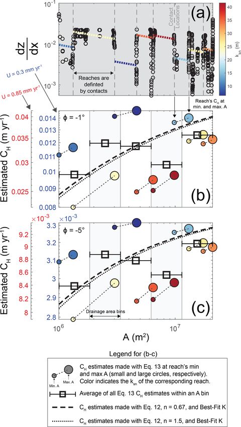
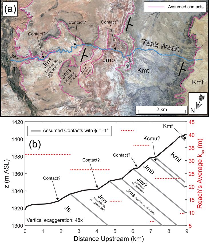
N. A. Mitchell and B. J. Yanites: Bedrock river erosion through dipping layered rocks                                                        725

Figure 1. Hanksville, UT, is a potential example of a landscape where contact migration significantly influences channel morphology.
(a) Google Earth imagery (© Google Earth) showing variations in channel steepness (ksn using a reference concavity of 0.5) near Hanksville.
These steepness values were obtained using TopoToolbox v2 (Schwanghart and Kuhn, 2010; Schwanghart and Scherler, 2014); more details
regarding the extraction of profile data are available in Sect. S1. The inset shows the locations of Hanksville, UT (yellow star), and the fluvial
terraces along the Fremont (red circle) that provide incision rate estimates of 0.3 to 0.85 mm yr−1 (Repka et al., 1997; Cook et al., 2009).

Figure 2. Conceptual models of bedrock river incision through layered stratigraphy. Here, only two rock types are shown: rock type 1 and
rock type 2. Panels (a, b) show a river with a contact dip (φ) of 0◦ . Panel (b) is at a later time than panel (a) to demonstrate how the contacts
gradually migrate upstream along the stream profile. Panel (c) shows a stream with contacts dipping in the upstream direction (φ < 0◦ ).
Panel (d) shows a stream with contacts dipping in the downstream direction (φ > 0◦ ).

https://doi.org/10.5194/esurf-9-723-2021                                                           Earth Surf. Dynam., 9, 723–753, 2021

726 N. A. Mitchell and B. J. Yanites: Bedrock river erosion through dipping layered rocks
oughly compared with observations from numerical models.
but present examples with θ = 0.3 and θ = 0.7 in the Supplement.
∗ The erodibilities of the medium layer (K , only present in scenario 2) and strong layer (K , present in all scenarios) are set relative to the reference weak erodibility (K ), as discussed in Sect. 2.2. We use θ = 0.5 in the main text
Table 1. Parameter space of the four model scenarios.
4
3
2
1
Scenario
Here, we use numerical models with which we can mea-
sure contact migration over time to pursue the following re-
search questions: (1) does the theory developed by Perne et
al. (2017) for river incision through horizontal strata accu-
dipping downstream
Two layers,
dipping upstream
Two layers,
zero dip
Three layers,
zero dip
Two layers,
Description
rately reflect observations from numerical models? (2) Does
the theory developed by Darling et al. (2020) for river in-
cision through nonhorizontal strata accurately reflect obser-
vations from numerical models? (3) What is the potential
for using these theoretical frameworks to estimate incision
M
model parameters like erodibility for real bedrock rivers?
By developing a new method for estimating kinematic wave
0.15 mm yr−1
0.15 mm yr−1
0.15 mm yr−1
0.3 mm yr−1
0.15 and
U (mm yr−1 )
speed, we will show that morphologic metrics like steepness
and contact dip can be used to estimate bedrock erodibility,
even where contact dips are nonzero. The dynamics of land-
scapes with layered rocks are increasingly shown to be quite
rich (Glade et al., 2017; Ward, 2019; Sheehan and Ward,
All H = 100 m
All H = 100 m
All H = 100 m
(4) HW = 150 and HS = 75 m
(3) HW = 75 and HS = 150 m, and
(2) HW = HS = 150 m,
(1) HW = HS = 100 m,
H (m)
2020a, b), and these landscapes offer valuable opportuni-
ties to compare expectations shaped by model results with
the unflinching testimony of the field. Our intention here
is to (1) further elucidate what we should expect from the
common form of the stream power model and (2) provide a
S
framework for quantifying rock strength from bedrock river
morphology. After developing this framework through the
use of numerical models, we demonstrate its application on
Tank Wash, one of the streams near Hanksville, UT (Fig. 1).
2 Methods
0.5, 1, 2.5, 5, 10, and 15◦
−15, −25, −35, and −45◦
−0.5, −1, −2.5, −5, −10,
0◦
0◦
φ (◦ )
To address the research questions outlined above, we model
one-dimensional river profiles using the stream power equa-
tion. We set up a series of model experiments to expand
upon previous work and generate a framework for extract-
ing quantitative information about erodibility in areas with
complex lithology. Table 1 summarizes the numerical model
scenarios we explore. We detail these models further below,
but at this point we emphasize that we examine four distinct
model scenarios: (1) models with two rock types and hori-
and 1.5
0.67
and 1.5
0.67
and 1.5
0.67
and 1.5
0.67
n
zontal contacts; (2) models with three rock types and hori-
zontal contacts; (3) models with two rock types and contacts
W
dipping in the upstream direction; and (4) models with two
n × 0.5
n × 0.5
n × 0.5
n × 0.5
m
rock types and contacts dipping in the downstream direction.
We use the first two model scenarios to test and further ex-
plore the framework developed by Perne et al. (2017) (i.e.,
and (3) 1.26 × 10⁻⁷
(1) 1.57 × 10⁻⁸ , (2) 4.44 × 10⁻⁸ ,
(3) 1.09 × 10⁻⁵ . For n = 1.5:
(2) 6.83 × 10⁻⁶ , and
For n = 0.67: (1) 4.29 × 10⁻⁶ ,
Reference KW (m1−2nθ yr−1 )
bedrock river incision through layered rocks when the con-
tact dip is zero), and we use the last two model scenarios
to test and further explore the framework developed by Dar-
ling et al. (2020) (i.e., bedrock river incision through layered
rocks when contact dips are nonzero). Note that both studies
are pertinent to river incision through horizontal or nonhor-
izontal units; we further describe in Sect. 2.4 why we focus
on a particular application for each study’s work.
∗
Earth Surf. Dynam., 9, 723–753, 2021 https://doi.org/10.5194/esurf-9-723-2021
N. A. Mitchell and B. J. Yanites: Bedrock river erosion through dipping layered rocks                                           727

2.1   Bedrock river erosion and morphology                          critical drainage area (0.1 km2 ) to occur where x = 20 km.
                                                                    We use a distance between stream nodes of dx = 5 m.
In this section, we present the basics of bedrock river erosion
                                                                       We present the resulting stream profiles as χ plots here
and the morphologic metrics we use to study it. We use a
                                                                    because χ –z space removes the influence of drainage area on
first-order upwind finite-difference scheme to represent the
                                                                    channel slope (Perron and Royden, 2013; Mudd et al., 2014):
stream power model (Howard and Kerby, 1983; Whipple and
Tucker, 1999):                                                            Zx            m/n
                                                                                   A0
                                                                    χ=                          dx,                              (4)
δz                   δz n                                                         A(x)
   = U − E = U − KAm      ,                                  (1)          xb
δt                   δx
                                                                    where χ is transformed distance upstream (L), xb is the po-
where z is elevation (L), t is time (T), U is rock-uplift           sition of base level (x = 0 m), and A0 is a reference drainage
rate L T−1 ), E is erosion rate (L T−1 ), K is erodibil-            area (here, taken as 1 km2 ).
ity (L1−2m T−1 ), A is drainage area (L2 ), x is distance up-          An effective method for comparing channel slopes and
stream (L), and both m and n are exponents. These exponents         contact dip φ is to use the slope of the contact in χ space,
reflect erosion physics and the scaling of both channel width       which we refer to as φχ :
and discharge with drainage area (Whipple and Tucker, 1999;
Lague, 2014). The ratio of m/n has been shown to influence                     dzcontact
                                                                    φχ =                 ,                                       (5)
river concavity (θ ) at steady state and uniform rock-uplift and                 dχ
erodibility (Tucker and Whipple, 2002). We use m/n = 0.5,           where zcontact is contact elevation (L) and χ is that of the
which falls within the expected range of m/n values (Whip-          stream node directly above the contact position in question.
ple and Tucker, 1999) and is consistent with many other stud-       Admittedly, comparing contact elevations with χ may be
ies (Farías et al., 2008; Gasparini and Whipple, 2014; Han          initially confusing, as χ is related to river elevations rather
et al., 2014; Mitchell and Yanites, 2019). We present sim-          than contact elevations. Utilizing the apparent contact dip in
ulations using m/n values of 0.3, 0.5, and 0.7 in the Sup-          χ space is advantageous, however, because it encapsulates
plement, however. Because slope exponent n strongly influ-          the influence of both drainage area and contact dip in real
ences bedrock river dynamics (Tucker and Whipple, 2002),            space. If one decides to utilize only drainage area or contact
we evaluate n values of 0.67 and 1.5. Although n is often as-       dip, then the influence of the excluded metric would not be
sumed to equal 1 (Farías et al., 2008; Fox et al., 2014; Goren      present in one’s analyses. Note that we will present φχ as
et al., 2014; Ma et al., 2020), we explain in Sect. 2.4 why we      dimensionless values (i.e., the change in elevation over the
do not evaluate models with n = 1.                                  change in transformed river distance), while we present con-
   For an equilibrated stream (dz/d = 0) with uniform prop-         tact dip φ in degrees.
erties, channel steepness ksn is related to the ratio of rock-
uplift rates to erodibility (Hack, 1973; Flint, 1974; Duvall et
                                                                    2.2    Defining the range of erodibility values
al., 2004; Wobus et al., 2006):
                       1/n                                        The contrast in erodibility (K) values between weak and
         dz m/n          U                                          strong layers is one of the most important controls on
ksn =        A     =            .                             (2)
         dx              K                                          bedrock river incision through layered stratigraphy, and we
                                                                    therefore explore this parameter space thoroughly. Select-
Equation (2) has shaped the focus of many studies in tec-
                                                                    ing K values for different simulations is not a simple mat-
tonic geomorphology (Wobus et al., 2006). Although this
                                                                    ter, however. The way erodibility influences river dynamics
framework is powerful, the streams we examine here have
                                                                    depends on the exponents m and n, so the effects of a 2-
spatially variable properties (i.e., K = f (x)). This distinction
                                                                    fold difference in K on both stream morphology and ero-
will cause variations in channel slope and steepness that are
                                                                    sion dynamics is not the same for n = 0.67 and n = 1.5.
not captured by Eq. (2), and we seek to further understand
                                                                    Furthermore, comparing K values is context-dependent. For
these variations in slope and channel steepness.
                                                                    example, K values could be selected to either (1) provide
   We use Hack’s law (Hack, 1957) to set each river’s
                                                                    a similar range of channel elevations (Beeson and McCoy,
drainage area:
                                                                    2020) or (2) allow similar timescales for transient adjustment
A(x) = C(` − x)h ,                                           (3)    (Mitchell and Yanites, 2019). Oftentimes, one cannot fulfill
                                                                    multiple such requirements when selecting erodibilities and
where x is distance upstream from the stream’s outlet, ` is         one must choose a specific approach. Because we examine
the length of the drainage basin (taken as 20.6 km), C is a         different n values here, we set the range of erodibility by
coefficient (L2−h ), and h is an exponent. We use C and h val-      considering slope patch migration rates (Royden and Perron,
ues of 1 m0.2 and 1.8, respectively. All streams are 20 km          2013).
long, so using ` = 20.6 km makes the rivers have a maximum             For the sake of concision, we summarize our approach for
drainage area of about 58 km2 . This ` value also causes the        setting erodibility values in Sect. S2. We use three reference

https://doi.org/10.5194/esurf-9-723-2021                                                        Earth Surf. Dynam., 9, 723–753, 2021
728                                     N. A. Mitchell and B. J. Yanites: Bedrock river erosion through dipping layered rocks

weak erodibilities (KW ) for each n value (Table 1). Using        is an important concept for this research because it is closely
these references KW values, we then calculate the erodibility     linked to contact migration along rivers. In this section, we
for the stronger layer (KS ) so it produces slope patch mi-       review the semi-analytical framework developed for kine-
gration rates that are a certain fraction (33 %, 50 %, 67 %,      matic wave speed when contact dip is zero (Perne et al.,
75 %, or 90 %) of those calculated for the weaker layer. We       2017).
chose this approach because (1) it allows us to objectively          Before we outline the semi-analytical framework devel-
and thoroughly explore K contrasts between weak and strong        oped in previous work, we provide a background on how
layers, and (2) the approach is consistent even with changes      erosion rate relates to kinematic wave speed. Contact migra-
in slope exponent n. While the erodibilities we use for dif-      tion can cause the erosion rates on either side of a contact to
ferent m and n values vary over several orders of magnitude,      change (Perne et al., 2017; Darling et al., 2020). One side of
K values corresponding to different drainage area m values        the contact can have an erosion rate below the base-level fall
have different dimensions (L1−2m T−1 ) and therefore cannot       rate, while the other side can have an erosion rate above it.
be directly compared. The K values we use are comparable          These erosion rate variations occur so that both sides of the
to those reported by Armstrong et al. (2021) (for those with      contact have the same horizontal retreat rate in the upstream
the same m values).                                               direction. This retreat rate is closely related to the concept
                                                                  of kinematic wave speed (CH ) (Rosenbloom and Anderson,
2.3   Recording contact migration rates
                                                                  1994):

                                                                                     n−1                                        n−1
We tracked and recorded contact positions over time in

                                                                            m   dz                                         E      n

our simulations. We recorded each contact’s position every        CH = KA                  = KAm/n ksn
                                                                                                    n−1
                                                                                                          = KA   m/n
                                                                                                                                       .   (6)
                                                                                dx                                         K
25 kyr, which is larger than model time step dt = 25 yr. Con-
tact migration rates are recorded for a total of 10 Myr for       Note that Eq. (6) suggests that CH has a power-law rela-
each simulation. Note that before we begin recording contact      tionship with drainage area (A). Although this is the general
migration rates, we run each simulation for a time period suf-    equation for kinematic wave speed, the challenge when con-
ficient to allow the range of river elevations to become con-     sidering rivers incising through layered rocks is what erosion
stant over time (i.e., a state of dynamic equilibrium). When      rate E is appropriate. Kinematic wave speed can be regarded
n < 1, we initialized the river elevations using the steepness    as the migration rate of signals along rivers. When consid-
(Eq. 2) for steady conditions and the strong layer’s erodibil-    ering such signals, geomorphologists usually think of base-
ity (ksn = (U/KS )1/n ). When n >1, we initialized the river      level fall due to tectonic activity (e.g., normal faulting) or
elevations using the steepness for steady conditions and the      drainage capture. The signals we are concerned with here,
weak layer’s erodibility (ksn = (U/KW )1/n ). After we initial-   however, are the erosional signals arising from contact mi-
ized the river elevations, the rivers needed some time to ad-     gration. Because the exposure of a new rock type can perturb
just from the initial conditions. Although the rivers quickly     erosion rates (Forte et al., 2016), even without changes in
arrive at morphologies like those shown in our conceptual         external drivers like base-level fall rate and climate, contact
model (Fig. 2), the river elevations can gradually increase or    migration is an autogenic perturbation. As erosion causes a
decrease before finally arriving at a consistent range of el-     contact to migrate upstream along a river, the autogenic sig-
evations (Figs. S1–S4 in the Supplement). The required ad-        nal persists and becomes a significant influence on river mor-
justment duration depends on both the initial conditions and      phology.
the rock-uplift rate used (i.e., the time for a contact to be        Perne et al. (2017) showed that when contacts are horizon-
uplifted across the fluvial relief). Streams in scenarios 1, 2,   tal (φ = 0◦ ), river reaches underlain by weak and strong rock
and 4 (Table 1) were given 50 Myr to adjust, while streams        types will have characteristic steepness values that reflect
in scenario 3 were given 100 Myr to adjust. These adjust-         the layers’ relative difference in erodibility. Surprisingly, the
ment times ensured that the streams in all simulations had        steeper reaches can sometimes be within the weaker rock
achieved a dynamic equilibrium (i.e., the range of elevations     type. Whether reaches in the strong or weak rock type are
became constant with time; Figs. S1–S4). We discuss our ap-       steeper depends on n, the parameter that controls how ero-
proach for measuring contact migration rates in our models        sion rate scales with channel slope (Eq. 1). The slope ex-
in Sect. S3.                                                      ponent n plays an important role in bedrock river incision
                                                                  through layered stratigraphy because it controls how kine-
2.4   Erosion and kinematic wave speed for horizontal
                                                                  matic wave speed scales with erosion rate (Eq. 6). The non-
      units
                                                                  linearity of Eq. (6) increases with |n − 1|. When n > 1, CH is
                                                                  directly proportional to E. When n < 1, CH is inversely pro-
Now, we delve further into (1) the erosion rate variations        portional to E. And when n = 1, CH is independent of E.
that occur during river incision through layered stratigra-       Strangely, this insensitivity of CH to E when n = 1 causes
phy and (2) how these erosion rate variations influence kine-     channels incising through layered rocks to consist only of
matic wave speed. We will show that kinematic wave speed          flat reaches and vertical steps (Fig. S5). The channel slopes

Earth Surf. Dynam., 9, 723–753, 2021                                                  https://doi.org/10.5194/esurf-9-723-2021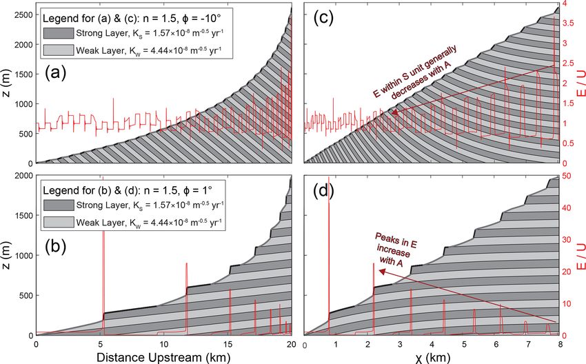
N. A. Mitchell and B. J. Yanites: Bedrock river erosion through dipping layered rocks                                             729

when n = 1 are either infinite or zero (infinite at the steps       we focus on the work of Darling et al. (2020) for nonzero
and zero in the flat reaches). Although this morphology has         contact dips. Although Darling et al. (2020) derived K ∗ by
been compared with waterfalls (Perne et al., 2017), waterfall       considering kinematic wave speeds, Perne et al. (2017) de-
dynamics are quite distinct (Lamb et al., 2007; Haviv et al.,       rived K ∗ by assuming that
2010; Scheingross and Lamb, 2017) and require a different
                                                                             ksnW A−m/n − tan(φ)

treatment. We do not intend to explicitly portray waterfalls        EW
                                                                         =                      ,                           (9)
here, and we therefore focus on models with n values of 0.67         ES      ksnS A−m/n − tan(φ)
and 1.5. We also do not assess simulations with n = 1 be-
cause we argue that Eq. (6) is not representative for those         where φ is the contact dip in degrees (positive when dip-
conditions. When n < 1, the weaker rock type has higher             ping in the downstream direction). The concept behind this
channel slopes and erosion rates (Perne et al., 2017). Con-         approach is that if the contact dip is high (e.g., vertical
versely, when n > 1 the strong rock type has higher channel         contacts that do not migrate horizontally), the right side of
slopes and erosion rates. We will use observations from our         Eq. (9) approaches 1. In that case, rearranging the equation
numerical models to further demonstrate why these behav-            would return us to the general expectations formed without
iors emerge.                                                        considering contact migration: that the erosion rate is the
   Because river incision through layered rocks in highly de-       same within each rock type (EW = KW Am |dz/dx|n = ES =
pendent on slope exponent n, simply evaluating the ratio of         KS Am |dz/dx|n ). If, however, the channel slopes are much
the weak and strong layers’ erodibilities (KW /KS ) is not an       higher than the contact slopes, then φ can be considered to
effective way to encapsulate the influence of contact migra-        go to zero. If φ = 0◦ , replacing the erosion rates in Eq. 9
tion. Instead, we use a term that is a function of the weak and     with the stream power equation (Eq. 1) and rearranging leads
strong erodibilities as well as slope exponent n. Darling et        to K ∗ (Eq. 7c). A similar approach was used by Imaizumi et
al. (2020) showed that if you consider weak and strong rock         al. (2015), albeit for the retreat of rock slopes rather than
types (with kinematic wave speeds CHW and CHS , erodibil-           rivers.
ities KW and KS , steepness values ksnW and ksnS , and ero-            The semi-analytical framework presented by Perne et
sion rates EW and ES , where the subscripts refer to weak           al. (2017) can be used to calculate kinematic wave speeds
and strong layers, respectively) and set the kinematic wave         for bedrock rivers incising through horizontal strata. We use
speeds equal to one another, you arrive at an equation Perne        measurements from our numerical models to test the accu-
et al. (2017) derived through a different approach. Because         racy of predictions made with their framework. To calculate
many readers will be unfamiliar with this work, we show the         the kinematic wave speed for a reach underlain by a strong
derivation in three parts.                                          layer, one must first solve for the erosion rate as (Perne et al.,
                                                                    2017)
CHW = KW Am/n ksn n−1
                   W
                      = CHS = KS Am/n ksn
                                       n−1
                                         S
                                                            (7a)                                            n
                                                                                                           1−n +1

              n−1                                                               HS               KS
KW

         ksnS                                                                    HW       +       KW
     =                                                      (7b)    ES = U                                          ,             (10)
KS       ksnW

                                                                                                  HS
                                                                                      1+          HW
              1          1
ksnW      KS n−1        KW 1−n
     =             =           = K∗                         (7c)
ksnS      KW            KS                                          where ES is the erosion rate in the stronger layer (L T−1 ),
                                                                    and HS and HW are the layer thicknesses (L) of the strong
We refer to this ratio as K ∗ . Note that if you express ksnW and   and weak layers, respectively. To calculate the weak erosion
ksnS in Eq. (7c) using Eq. (2) (e.g., ksnW = (EW /KW )1/n ),        rate (EW ) for a contact dip of zero, the strong and weak in-
you will also find that                                             dices in Eq. (10) can simply be reversed. The kinematic wave
       EW                                                           speed within one layer can then be estimated by inserting
K∗ =      ,                                                  (8)    Eq. (10) into the general equation for kinematic wave speed
       ES
                                                                    (Eq. 6). Note that Perne et al. (2017) derived Eq. (10) by
where EW and ES are the erosion rates in the weak and strong        assuming that the average erosion at each point along the
layers, respectively. Even though K ∗ represents the contrast       stream over time must balance the rock-uplift rate (U ). To
in erosion or steepness between weak and strong rock types          understand the concept behind this approach, first consider a
when the contact dip is zero, we will show that K ∗ is still an     reach that is underlain by one rock type and that is eroding at
effective metric for erodibility contrasts when contact dips        a rate above U . As erosion causes the contacts defining that
are nonzero (in the form (KW /KS )1/(1−n) ). Although we fo-        reach to migrate upstream over time, the reach creates an im-
cus on the approach of Darling et al. (2020) for nonzero con-       balance between the river’s erosion rate and rock-uplift rate.
tact dips, it can be applied to river incision through horizontal   After the reach migrates past one position, however, its mi-
units (by setting the contact slope to zero). The approach of       gration is followed by a reach in another rock type. This rock
Darling et al. (2020) then becomes the same as that of Perne        type would have an erosion rate below the rock-uplift rate,
et al. (2017) (i.e., both studies derived Eq. 7c), however, so      and the passage of this low-erosion reach restores the balance

https://doi.org/10.5194/esurf-9-723-2021                                                          Earth Surf. Dynam., 9, 723–753, 2021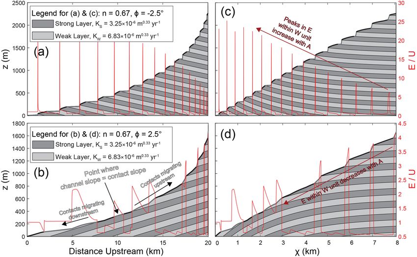
730                                     N. A. Mitchell and B. J. Yanites: Bedrock river erosion through dipping layered rocks

over time between rock uplift and erosion. Perne et al. (2017)     for the kinematic wave speed as
based this perspective on observations from their numeri-                               n
                                                                                   dz
cal models; despite oscillations in channel slope as contacts             KW Am    dx                          Am U
migrate upstream, the rivers reached a dynamic equilibrium         CH =                     =         1/n                         ,   (12)
                                                                           dz
such that the range of elevations was constant over time. This             dx   − tan(φ)           U
                                                                                                               A−m/n       − tan(φ)
                                                                                                   KW
dynamic equilibrium suggests that erosion and rock uplift do
balance each other over a sufficient time interval (i.e., the      where the weak layer is assumed to erode at rock-uplift
time for reaches in both rock types to migrate past a posi-        rate U . Note that Eq. (12) suggests that when φ < 0◦ (dip-
tion). Given the assumptions involved in the derivation of         ping upstream), CH will be lower (i.e., the denominator
Eq. (10), however, we will use measurements from our nu-           will increase). When φ > 0◦ (dipping downstream), CH will
merical models to test its accuracy.                               be higher (i.e., the denominator will decrease). Although
   To test if Eqs. (7)–(10) are accurate across different          CH usually increases as a power-law function of drainage
m/n values, we also assess six additional simulations: two         area (Eq. 6), Eq. (12) also suggests that nonzero contact dips
with m/n = 0.3, two with m/n = 0.5, and two with m/n =             will cause a departure from the power-law relationships typi-
0.7. For each m/n value, the two simulations use n values          cally expected (i.e., in a log–log plot of CH vs. drainage area,
of either 0.67 or 1.5. Because each simulation uses differ-        the data will no longer follow a linear trend). While Perne
ent m values, these simulations require a different approach       et al. (2017) showed that the erosion rate of the weak layer
for setting erodibility values. We discuss this approach in        changes when contact dip is zero, Darling et al. (2020) as-
Sect. S4.                                                          sumed that the weak layer erodes at the base-level fall rate.
                                                                   Darling et al. (2020) focused on scenarios with n > 1; be-
                                                                   cause the strong layer is the less steep layer when n < 1, we
                                                                   will use the parameters of the strong layer (KS ) in Eq. (12)
2.5   Erosion and kinematic wave speed for nonhorizontal           when n < 1.
      units                                                           In addition to Eq. (12), we present an alternative method
                                                                   to estimate kinematic wave speed from channel steepness.
When units have nonzero dips, the dynamics between erosion
                                                                   We have essentially modified the approach of Darling et
rate and kinematic wave speed change entirely (Darling et
                                                                   al. (2020) to utilize observed channel steepness. The ap-
al., 2020). To evaluate how bedrock river erosion rates vary
                                                                   proach remains applicable whether the contact dip is zero or
with contact dip, we fit multilinear regressions to our model
                                                                   nonzero, and although it utilizes a base-level rate (U ) it is not
results in the form
                                                                   based on assumptions regarding the erosion rate within each
                                                                   layer. Kinematic wave speed CH for a reach underlain by one
EW
   = f K ∗ , ln(|φχ |) ,                                           rock type can be estimated as

                                                           (11)
U
                                                                             U
                                                                                                n
                                                                             n
                                                                            ksn  Am ksn A−m/n                  U
where EW /U is the average erosion rate of the weak unit           CH =
                                                                                 −m/n
                                                                                      n           =
                                                                                                           −m/n
                                                                                                                n          , (13)
                                                                            ksn A        − tan(φ)     ksn A        − tan(φ)
normalized by rock-uplift rate, K ∗ is a metric for the erodi-
bility contrasts between weak and strong layers (Eq. 7c), and      where ksn is the average steepness observed for the reach
φχ is the contact dip in χ space (Eq. 5). The purpose of this      spanning the layer in question. We estimate the K value in
approach is to demonstrate how erosion rates change with           Eq. (13) as U/ksn  n ; this approach assumes the reach is equi-

drainage area, contact dip (both of which influence φχ ), and      librated to U and previous work (Forte et al., 2016; Perne et
contrasts in rock strength. We take the average EW /U and          al., 2017; Darling et al., 2020) suggests that this assumption
ln(|φχ |) values within 10 drainage area bins spaced loga-         can be incorrect. The advantage of this approach, however,
rithmically from the highest to lowest drainage areas. Uti-        lies in taking the average of Eq. (13) estimates from mul-
lizing the logarithm of |φχ | is effective because this drainage   tiple rock types. For example, the Eq. (13) CH estimates for
area proxy aids in portraying the power-law relationships sur-     one rock type will be too high, while the CH estimates for the
rounding drainage area in the stream power model (Eq. 1).          other rock type will be too low. By taking the average of both
Excluding the influence of contact dip by using drainage area      estimates, the deviations in erosion rate balance each other
instead of ln(|φχ |) would, for example, provide only scat-        out and provide an accurate estimate of CH . Importantly,
ter rather than the three-dimensional relationships we will        this approach can then be combined with that of Darling et
demonstrate between EW /U , K ∗ , and ln(|φχ |). For these         al. (2020) (Eq. 12). By utilizing Eqs. (12) and (13) together,
analyses, we only use erosion rates from the final model time      one can compare CH estimates based only on quantifiable
step (rather than values over the entire 10 Myr duration).         metrics (U , ksn , and φ in Eq. 13) and CH estimates calculated
   Now, we present the framework for kinematic wave speeds         using a specified erodibility (Eq. 12). We will show that this
along bedrock rivers incising through nonhorizontal strata.        combination can allow the estimation of erodibility for real
Darling et al. (2020) used geometric considerations to solve       streams, like those near Hanksville, UT (Fig. 1). We describe

Earth Surf. Dynam., 9, 723–753, 2021                                                    https://doi.org/10.5194/esurf-9-723-2021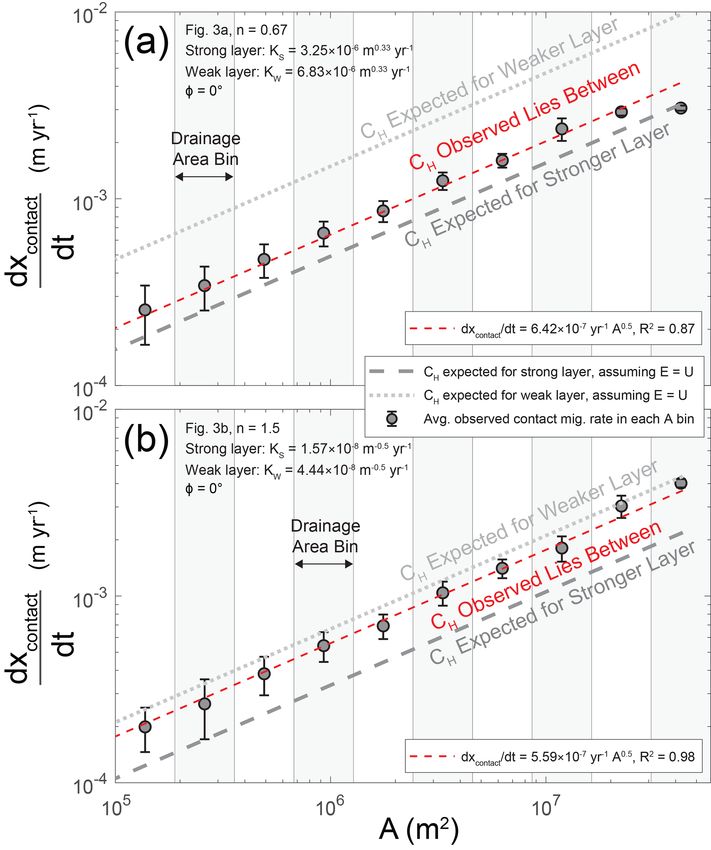
N. A. Mitchell and B. J. Yanites: Bedrock river erosion through dipping layered rocks                                       731

this combination further below, after we provide more details      number of free variables (ν = 1 here, as we only vary K in
regarding the application of Eq. (13).                             Eq. 12), simi and obsi are the CH estimates from Eqs. (12)
   To estimate CH with Eq. (13), we utilize the following          and (13) in each drainage area bin, respectively, and “toler-
procedure: (1) create bins defined by drainage area values,        ance” is taken as 1 m yr−1 . Note that we take the obsi val-
with 10 bins spaced logarithmically from the lowest to the         ues as the average CH estimates made with Eq. (13); we
highest drainage areas; (2) for each drainage area bin, take       made this decision because (1) CH values from Eq. (13) are
the average steepness (ksn ) within each rock type; (3) using      based on measured steepness, (2) we thoroughly compare our
the average steepness for each rock type, calculate CH with        Eq. (13) estimates with contact migration rates measured in
Eq. (13); and (4) take the average of the CH estimates from        our models, and (3) measured contact migration rates would
both rock types in each drainage area bin. Note that this ap-      not be available for a real stream. Although tolerance can
proach requires an independent estimate of rock-uplift rate U      be set in such a way that simulations with X 2 values under
(or base-level fall rate) and contact dip φ. Due to the data       some threshold are defined as acceptable, we do not use X2
limitations for real streams, we will compare contact migra-       in that manner here. Instead, we show the X 2 values for all
tion rates measured in our models with Eq. (13) CH estimates       Eq. (12) estimates (using 200 K values spaced logarithmi-
that use only ksn values from the final model time step of         cally from 10−9 to 10−4 m1−2nθ yr−1 ) and focus on the K
each simulation. We show Eq. (13) estimates using the en-          with the lowest X 2 as the best-fit K (i.e., this would be the
tire 10 Myr of recorded ksn values for each simulation in the      best estimate for the stream’s erodibility). Varying the tol-
Supplement, however. Equation (12) does not use ksn values         erance would scale the magnitudes of all X 2 values, but it
recorded over time. Note that we bin results by drainage area      would not alter which K value corresponds to the lowest X 2 .
mainly for visual clarity in our figures. To test the influence    We compare the best-fit K values in each simulation with the
of our binning approach, we present a figure in the Supple-        simulation’s weak and strong erodibilities (KW and KS ).
ment in which we use 20 drainage area bins instead of 10.             Although we use this approach to search for the K value
   To further examine the influence of different m/n values,       that produces the best agreement between the Eq. (12)
we also assess six additional simulations with a contact dip φ     and (13) estimates of CH (the Eq. 12 estimates use a range
of −2.5, n values of 0.67 or 1.5, and m/n values of 0.3, 0.5,      of K and the Eq. 13 estimates use measured ksn ), we do
or 0.7. The approach for setting erodibility values in these       not perform such a search for the slope exponent n value.
simulations is discussed in Sect. S4. Although we examine          In each simulation, we calculate Eq. (12) and (13) estimates
a wider range of contact dips in our main simulations (Ta-         of CH using the n value enforced in each simulation. Using
ble 1), these additional simulations are meant to be a limited     the correct m and n values is crucial for estimating the ap-
selection of examples that demonstrate the influence of dif-       propriate magnitude and dimensions of erodibility, but our
ferent m/n values on bedrock river incision through layered        intention here is only to show how accurately K can be es-
rocks.                                                             timated. Using the incorrect n to estimate the K used in a
   Now, we describe how we combine the framework devel-            simulation would involve comparing erodibilities with differ-
oped by Darling et al. (2020) (Eq. 12) with our approach           ent dimensions (if m/n remains constant). As we discussed
(Eq. 13) in the evaluation of our numerical models. Note           in Sect. 2.2, comparing K values is context-dependent. We
that we perform this comparison to test how well it can re-        could compare the fluvial relief values expected for differ-
cover erodibility values from river morphology in a numer-         ent K, or we could compare slope patch migration rates.
ical model; establishing this accuracy is important because        Attempting to fully explore such considerations, however,
we apply similar analyses to Tank Wash near Hanksville, UT         would negatively impact the focus and brevity of this study.
(Fig. 1). We describe our analysis of Tank Wash in Sect. 2.6       Furthermore, we perform these analyses on our numerical
below. To test the effectiveness of this approach in the nu-       models to inform our analysis of Tank Wash (Sect. 2.6), and
merical models, we compare the average Eq. (13) CH esti-           our analysis of Tank Wash includes the consideration of mul-
mate within each drainage area bin with Eq. (12) CH values         tiple n values.
calculated using the enforced contact dip (φ) and slope expo-
nent (n) as well as a wide range of erodibilities (K, 200 val-     2.6   Analysis of Tank Wash
ues spaced logarithmically from 10−9 to 10−4 m1−2nθ yr−1 ,
where θ = 0.5). We compare the two sets of kinematic wave          We explore the behavior of these rivers in numerical mod-
speed estimates with the X2 misfit function (Jeffery et al.,       els to develop a framework for quantifying erodibility from
2013):                                                             bedrock river morphology. After presenting our numerical
                                                                   model results, we apply the developed framework to Tank
            N
                simi − obsi 2

  2    1   X                                                       Wash near Hanksville, UT (Fig. 1). We use Google Earth im-
X =                           ,                            (14)
    N −ν −1 i    tolerance                                         agery and the nearby 1 : 62k geologic map of the San Rafael
                                                                   Desert Quadrangle (which includes the same units; Doelling
where N is the number of observations being compared (up           et al., 2015) to infer the map-view positions of contacts near
to 10 for average values in the 10 drainage area bins), ν is the   Tank Wash. We then infer the contact locations along Tank

https://doi.org/10.5194/esurf-9-723-2021                                               Earth Surf. Dynam., 9, 723–753, 2021
732                                      N. A. Mitchell and B. J. Yanites: Bedrock river erosion through dipping layered rocks

Wash’s longitudinal profile by considering both the inferred        lations that use different m/n values (Sect. S4) will allow us
map-view contacts and changes in the stream’s steepness             to consider the influence of varying m/n.
(Fig. 1b). Channel profile data are taken from 10 m digi-
tal elevation models (DEMs) provided by the United States
Geological Survey. We extracted profile data using Topo-            3     Results
Toolbox v2 (Schwanghart and Kuhn, 2010; Schwanghart and
Scherler, 2014); more details regarding the extraction and          3.1    Scenario 1: two rock types with φ = 0◦
processing of profile data are available in Sect. S1 in the Sup-
plement. There are no contact dip measurements available in         In this section, we present the results for scenario 1 of our
the vicinity of Tank Wash, but based on regional geology, the       numerical models (Table 1). These simulations use two rock
contact dips are likely relatively low. For example, Ahmed et       types (weak and strong) with contact dips of 0◦ . We use the
al. (2014) reported a dip of 3◦ to the west in an area just north   results for scenario 1 to (1) further explain the dynamics of
of Tank Wash. We evaluate contact dips of −1 and −5◦ (dip-          bedrock river incision through flat-lying strata and (2) test
ping in the upstream direction) because the geologic maps           and further explore the semi-analytical framework developed
(Doelling et al., 2015) and imagery available in the area sug-      by Perne et al. (2017).
gest that contact dips are likely relatively low. Furthermore,         Figure 3 shows long profiles (Fig. 3a and b) and χ plots
our results will demonstrate the effect of contact dip on these     (Fig. 3c and d) for two simulations of bedrock rivers under-
analyses in a manner that enables extrapolation (e.g., consid-      lain by alternating weak and strong rock layers. The simu-
ering if the dip was −3 or −10◦ ). Although this approach is        lation in Fig. 3a and c has n = 0.67 and K ∗ of ∼ 9.5 (weak
far from ideal, our intention here is only to demonstrate how       layer’s erodibility K is ∼ 2.1 times higher than the strong
one could apply the developed framework to real streams.            layer’s K), while the simulation in Fig. 3b and d has n = 1.5
Any accurate analyses would require detailed field surveys,         and K ∗ of ∼ 0.13 (weak layer’s K is ∼ 2.8 times higher than
and such endeavors could be the focus of future work.               the strong layer’s K). Note that the erosion rates normalized
   After identifying the potential contacts, we (1) divide Tank     by rock-uplift rate (E/U ) are shown as red lines. Like the
Wash’s profile into reaches separated by the inferred con-          streams near Hanksville, UT, and those simulated by Perne
tact locations and (2) use the average steepness of each reach      et al. (2017), these streams have a stepped appearance. As we
to estimate kinematic wave speed (CH ) values according to          discussed in Sect. 2.4, when n < 1 (Fig. 3a and c) reaches un-
Eq. (13). These CH estimates are made twice for each reach:         derlain by the weaker rocks have higher channel slopes and
once at the minimum drainage area and once at the maxi-             erosion rates. When n > 1 (Fig. 3b and d), reaches underlain
mum. We then take the average of all CH values within five          by the stronger rocks have higher channel slopes and erosion
drainage area bins spaced logarithmically from the lowest to        rates. To explain why the erosion rate variations in Fig. 3 oc-
highest drainage areas. To explore what erodibilities could         cur, we now examine the contact migration rates within each
yield similar results (given the assumed contact dips evalu-        of these simulations.
ated), we compare the average CH estimates from our ap-                Figure 4a and b show contact migration rates (dxcontact /dt)
proach (Eq. 13) with a range of predictions from the Darling        versus drainage area (A) for the simulations in Fig. 3a
et al. (2020) portrayal of kinematic wave speed (Eq. 12). We        and b, respectively. We show the average measured con-
perform this comparison with the X2 misfit function (Eq. 14).       tact migration rates (gray circles with black outlines) within
We evaluate a large range of K for Tank Wash (200 val-              10 drainage area bins; the vertical bars for each circle repre-
ues spaced logarithmically from 10−8 to 10−2 m1−2nθ yr−1 ,          sent the standard deviation of dxcontact /dt within the corre-
where θ = 0.5). Because Eq. (12) requires an estimated rock-        sponding drainage area bin. In Fig. 4a and b, the light gray
uplift rate (i.e., base-level fall rate), we use the range of in-   dotted line represents the kinematic wave speed (Eq. 6) ex-
cision rates from the cosmogenic dating of fluvial terraces         pected if only the weak layer was present and all erosion rates
along the nearby Fremont River (0.3 to 0.85 mm yr−1 ; Repka         were equal to the rock-uplift rate. Similarly, the dark gray
et al., 1997; Cook et al., 2009; red circle in Fig. 1a). Inci-      dashed line shows the kinematic wave speed expected if only
sion rates from terraces are not necessarily representative of      the strong layer was present and all erosion rates were equal
base-level fall rates, but there are no other constraints in the    to the rock-uplift rate. If only one rock type was present, one
area. Importantly, our results will enable us to consider how       could think of these wave speeds as the upstream migration
the estimated erodibility would scale with the assumed base-        rate of bedding planes within the units, as rock uplift carries
level fall rate (i.e., considering how the erodibility would        the units up the stream profile. The measured contact migra-
change if the incision rate was only 0.15 mm yr−1 instead           tion rate lies somewhere between these two end-members.
of 0.3 mm yr−1 ). For this analysis of Tank Wash, we eval-          This finding is highlighted by the dashed red lines, which are
uate n values of 0.67 and 1.5 and assume that m/n = 0.5.            power-law functions fit between the observed contact migra-
Although a wide range of n values are possible, our inten-          tion rates and the drainage areas at the center of each bin (as-
tion is to focus on a limited number of examples for which          suming a drainage area exponent of m/n, which is 0.5 here).
n is less than or greater than 1. Similarly, the example simu-      While the fact that contact migration rates fall between the

Earth Surf. Dynam., 9, 723–753, 2021                                                   https://doi.org/10.5194/esurf-9-723-2021
N. A. Mitchell and B. J. Yanites: Bedrock river erosion through dipping layered rocks                                               733

Figure 3. Longitudinal profiles (a, b) and χ plots (c, d) for two different simulations. The simulation in (a) and (c) has slope exponent
n values of 0.67, while the simulation in (b) and (d) has n = 1.5. Layer thickness H and rock-uplift rate U are 100 m and 0.15 mm yr−1 in
both simulations, respectively.

two extremes shown in each panel may sound straightfor-                case the strong unit slows down the contact’s migration. The
ward, the reason for this result is not intuitive.                     stretch zone in the strong unit is then replaced by a reach
   These dynamics occur because channel slopes on both                 of low steepness. This transition occurs because the combi-
sides of the contact interact to drive the system towards equal        nation of undercutting by the weak unit and resistance from
retreat rates and kinematic wave speeds (CH ) across the con-          the strong unit leads (1) to higher channel slopes and erosion
tact. For example, consider a contact with a weak unit situ-           rates within the weak unit and (2) lower channel slopes and
ated beneath a strong unit. The stream segment in the weak             erosion rates within the strong unit (i.e., due to lengthening
unit may initially erode at a higher rate, undercutting the            of each reach within the strong unit).
strong unit and forcing the contact further upstream. Impor-              Although we discussed these dynamics in qualitative terms
tantly, the response of the strong unit depends on slope ex-           above, we will now we discuss them with a stronger fo-
ponent n in the stream power model. When n > 1, higher                 cus on contact migration rates (Fig. 4) and kinematic wave
erosion rates in the weak unit will cause a consuming knick-           speed (CH ). To maintain equal retreat rates, reaches within
point (Royden and Perron, 2013) to migrate into the strong             the weaker layer develop a lower CH value relative to what
unit situated above. The strong unit responds rapidly in this          would be expected if they were eroding at the rock-uplift
case, keeping pace with the weak unit by eroding at a higher           rate (dotted gray lines in Fig. 4). Conversely, reaches within
rate. This response is so effective that the contact’s migration       the stronger layer develop a higher CH value. When n < 1,
leads to a reduction in channel slope within the weak unit             Eq. (6) shows that CH is inversely proportional to erosion
(i.e., lengthening each reach within the weak unit), decreas-          rate E. Because of this relationship, reaches in the weak
ing the weak unit’s erosion rate. When n < 1, however, there           layer achieve a lower CH (i.e., slow down) by increasing E
is no consuming knickpoint. Instead, the initially higher ero-         when n < 1. Similarly, reaches in the strong unit achieve
sion rate in the weak unit causes an erosional signal that mi-         a higher CH (i.e., speed up) by decreasing E when n < 1.
grates more slowly through the strong unit above. A stretch            Due to such behaviors, when n < 1 the stream has higher
zone (Royden and Perron, 2013) initially forms at the base             steepness and erosion rates within the weak unit and sub-
of the strong unit (i.e., a convex-upwards knickzone). Instead         dued steepness and erosion rates within the strong unit. The
of rapidly adjusting to keep pace with the weak unit, in this          opposite is true when n > 1; reaches in the weak unit ob-

https://doi.org/10.5194/esurf-9-723-2021                                                     Earth Surf. Dynam., 9, 723–753, 2021
734                                       N. A. Mitchell and B. J. Yanites: Bedrock river erosion through dipping layered rocks

Figure 4. Contact migration rates (dxcontact /dt) vs. drainage area (A) for (a) the simulation shown in Fig. 3a and c and (b) the simulation
shown in Fig. 3b and d.

tain a lower CH value (i.e., slow down) by decreasing E, and            are horizontal, contact migration rates reflect the kinematic
reaches in the strong unit obtain a higher CH value (i.e., speed        wave speeds of the surrounding stream reaches. Furthermore,
up) by increasing E.                                                    erosion rate variations like those in Fig. 3 occur so that kine-
   To assess if the theory developed by Perne et al. (2017) is          matic wave speeds are equal on either side of a contact, al-
applicable across the parameter space explored in scenario 1,           lowing kinematic wave speed to consistently increase with
we compared kinematic wave speeds calculated with Eqs. (6)              drainage area as shown in Fig. 4.
and (10) with contact migration rates (dxcontact /dt) measured             Figures S6–S10 show the results for the six additional
in our models (Fig. 5). Note that in Fig. 5, both metrics               simulations with horizontal contacts and different m/n val-
have been normalized by drainage area raised to the m/n; as             ues (0.3, 0.5, or 0.7). Even though the dimensions of
shown in Fig. 4, contact migration rates change with drainage           erodibility depend on m, which varies across these simu-
area. Despite all of the changes in parameters like erodibili-          lations (Figs. S6 and S7), the simulations with the same
ties, layer thicknesses, and rock-uplift rates in scenario 1 (Ta-       n value (0.67 or 1.5) were set up to have the same K ∗ value.
ble 1), the kinematic wave speeds predicted using the frame-            Because the simulations have the same K ∗ value, the vari-
work from Perne et al. (2017) (Eqs. 6 and 10) serve as ex-              ations in erosion rate are roughly the same. These findings
cellent portrayals of the contact migration rates in our nu-            suggest that the nondimensional parameter K ∗ is represen-
merical models. These findings indicate that when contacts              tative of the variations in channel steepness and erosion rate

Earth Surf. Dynam., 9, 723–753, 2021                                                        https://doi.org/10.5194/esurf-9-723-2021
N. A. Mitchell and B. J. Yanites: Bedrock river erosion through dipping layered rocks                                            735

                                                                      tional rock type will adjust to allow for a consistent trend in
                                                                      kinematic wave speed across the profile. Here, the medium
                                                                      layer is the additional rock type relative to the simulations in
                                                                      scenario 1. For example, Fig. S11 shows the contact migra-
                                                                      tion rates for the simulations in Fig. 6a and b; despite differ-
                                                                      ing erodibilities, contact migration rates and CH increase as a
                                                                      power-law function of drainage area. The fact that steepness
                                                                      ratios and erosion rate ratios are both well represented by K ∗
                                                                      (Fig. 6c) follows from Eqs. (7c) and (8), which were derived
                                                                      by setting the kinematic wave speeds within two rock types
                                                                      equal to each other.

                                                                      3.3     Scenarios 3 and 4

                                                                      3.3.1    General morphologic results of nonzero contact
                                                                               dips
Figure 5. Estimated kinematic wave speeds (CH ) and measured
contact migration rates (dxcontact /dt) for all simulations in sce-   Before we test the framework developed by Darling et
nario 1 (Table 1). The low-U scenarios have U = 0.15 mm yr−1 ,        al. (2020) for bedrock river incision through nonhorizon-
while the high-U scenarios have U = 0.3 mm yr−1 . Symbol size         tal strata, we present example simulations demonstrating the
represents the reference weak erodibility used (KW ; Table 1).        general morphologic implications of nonzero contact dips.
                                                                      Our simulations indicate that river morphology can be signif-
                                                                      icantly altered by even slight changes in contact dip (Figs. 7
caused by rock strength contrasts (Eqs. 7c, 8, and 10) even           and 8). Figure 7 shows the long profiles (Fig. 7a and b) and
when drainage area exponent m varies. Furthermore, the con-           χ plots (Fig. 7c and d) for two simulations with n = 0.67
tact migration rates measured in these additional simulations         and the same erodibility values (K) used in Fig. 3a, but with
are still well represented by the kinematic wave speeds cal-          slight dips to the contacts. One simulation has contacts dip-
culated with the framework of Perne et al. (2017) (Fig. S10).         ping upstream at 2.5◦ (φ = −2.5◦ ; Fig. 7a and c), and the
                                                                      other simulation has contacts dipping downstream at 2.5◦
3.2   Scenario 2: three rock types with φ = 0◦                        (φ = 2.5◦ ; Fig. 7b and d). Although the strong and weak
                                                                      erodibilities in Fig. 7 are the same as those in Fig. 3a, the
In this section, we examine the results for scenario 2 (Ta-           morphologies of these streams are quite distinct. For exam-
ble 1). Like scenario 1, scenario 2 only considers horizon-           ple, although the simulations use the same erodibilities, rock-
tal contacts (contact dip φ = 0◦ ). Unlike scenario 1, how-           uplift rates, layer thicknesses, and drainage areas, the maxi-
ever, scenario 2 utilizes three rock types (weak, medium, and         mum river elevations in Figs. 3a, 7a, and 7b are about 1800,
strong). Our intention is to test if the equations presented by       2300, and 1700 m, respectively. Indeed, such pronounced
Perne et al. (2017) still hold when there are more than two           changes in river erosion and morphology for deviations in
rock types because real streams usually incise through strata         contact dip of only 2.5◦ away from horizontal bedding planes
that are far more complicated than those considered in sce-           highlight the importance of contact dip in river morphology.
nario 1.                                                              Note that in the χ plots in Fig. 7, the apparent contact dip in
   Figure 6a and b show long profiles with three rock types           χ space (φχ ; Eq. 5) varies along the profile. When contacts
of equal thickness (100 m) and n values of 0.67 (Fig. 6a) and         dip upstream (φ < 0◦ ) φχ is negative, and when contacts dip
1.5 (Fig. 6b). Figure 6c shows ratios of the average steep-           downstream (φ > 0◦ ) φχ is positive. In both χ plots, how-
ness values (ksn ) and erosion rates (E) within different rock        ever, the absolute value of φχ approaches zero with increas-
types (e.g., ksn of weak layer / ksn of strong layer) for all sim-    ing χ (i.e., the contacts seem to bend and almost become
ulations in scenario 2. The purpose of Fig. 6c is to test if          horizontal).
Eqs. (7c) and (8) (Perne et al., 2017) are still accurate when           The two simulations in Fig. 8 have n = 1.5 and the same
there are three rock types instead of two. Because the steep-         erodibility (K) values used in Fig. 3b, but with nonzero con-
ness and erosion ratios in Fig. 6c follow a 1 : 1 relationship        tact dips. Because we examined simulations with the same
with K ∗ , these results are consistent with Eqs. (7c) and (8).       absolute contact dips in Fig. 7 (|φ| = 2.5◦ ), we now show
   These results suggest that the theory developed by Perne et        simulations with dissimilar contact dips: Fig. 8a and c have
al. (2017) for bedrock river incision through horizontal strata       contacts dipping 10◦ upstream (φ = −10◦ ), while the simu-
still applies when there are more than two rock types. When           lation in Fig. 8b and d has contacts dipping 1◦ downstream
there is an additional rock type (e.g., more than three litholo-      (φ = 1◦ ). These two simulations with n = 1.5 (Fig. 8) also
gies), the channel slopes and erosion rates within the addi-          have distinct morphologies relative to similar simulations

https://doi.org/10.5194/esurf-9-723-2021                                                   Earth Surf. Dynam., 9, 723–753, 2021
You can also read