Bias Mimicking: A Simple Sampling Approach for Bias Mitigation
←
→
Page content transcription
If your browser does not render page correctly, please read the page content below
Bias Mimicking: A Simple Sampling Approach for Bias Mitigation

                                                                        Maan Qraitem1 , Kate Saenko1,2 , Bryan A. Plummer1
                                                                         1
                                                                           Boston University 2 MIT-IBM Watson AI Lab
                                                                                {mqraitem,saenko,bplum}@bu.edu
arXiv:2209.15605v8 [cs.CV] 27 Apr 2023

                                                                 Abstract

                                             Prior work has shown that Visual Recognition datasets
                                         frequently underrepresent bias groups B (e.g. Female)
                                         within class labels Y (e.g. Programmers). This dataset bias
                                         can lead to models that learn spurious correlations between
                                         class labels and bias groups such as age, gender, or race.
                                         Most recent methods that address this problem require sig-
                                         nificant architectural changes or additional loss functions
                                         requiring more hyper-parameter tuning. Alternatively, data
                                         sampling baselines from the class imbalance literature (e.g.
                                         Undersampling, Upweighting), which can often be imple-
                                         mented in a single line of code and often have no hyper-
                                         parameters, offer a cheaper and more efficient solution.
                                         However, these methods suffer from significant shortcom-
                                         ings. For example, Undersampling drops a significant part
                                         of the input distribution per epoch while Oversampling re-
                                         peats samples, causing overfitting. To address these short-
                                         comings, we introduce a new class-conditioned sampling              Figure 1. Comparison of sampling approaches for mitigating bias
                                         method: Bias Mimicking. The method is based on the obser-           of class labels Y (Hair Color) toward sensitive group labels B
                                         vation that if a class c bias distribution, i.e. PD (B|Y = c)       (Gender). (a) illustrates Undersampling/Oversampling methods
                                         is mimicked across every c′ ̸= c, then Y and B are statisti-        that drop/repeat samples respectively from a dataset D per epoch
                                         cally independent. Using this notion, BM, through a novel           and thus ensure that PD (Y |B) = PD (Y ). However, dropping
                                         training procedure, ensures that the model is exposed to            samples hurt the model’s predictive performance, and repeating
                                                                                                             samples can cause overfitting with over-parameterized models like
                                         the entire distribution per epoch without repeating samples.
                                                                                                             neural nets [35]. (b) shows our Bias Mimicking approach which
                                         Consequently, Bias Mimicking improves underrepresented              subsamples D and produces three variants. Each variant, denoted
                                         groups’ accuracy of sampling methods by 3% over four                as dc ⊂ D, preserves class c samples (i.e. mimicked class) and
                                         benchmarks while maintaining and sometimes improving                mimics the bias of class c in each c′ ̸= c. This mimicking pro-
                                         performance over nonsampling methods. Code: https:                  cess, as we show in our work, ensures that Pdc (Y |B) = Pdc (Y ).
                                         //github.com/mqraitem/Bias-Mimicking                                Moreover, by using each dc separately to train the model, we ex-
                                                                                                             pose it to all the samples in D per epoch, and since we do not
                                                                                                             repeat samples in each dc , our method is less prone to overfitting.
                                         1. Introduction
                                            Spurious predictive correlations have been frequently            model’s predictions of input samples from their member-
                                         documented within the Deep Learning literature [34, 38].            ship to bias groups. Previous research efforts have primar-
                                         These correlations can arise when most samples in class             ily focused on model-based solutions. These efforts can be
                                         a c (e.g. blonde hair) belong to a bias group s (e.g. fe-           mainly categorized into two directions 1) ensemble-based
                                         male). Thus, the model might learn to predict classes by us-        methods [35], which introduce separate prediction heads for
                                         ing their membership to their bias groups (e.g. more likely         samples from different bias groups 2) methods that intro-
                                         to predict blonde hair if a sample is female). Mitigating           duce additional bias regularizing loss functions and require
                                         such spurious correlations (Bias) involves decorrelating the        additional hyper-parameter tuning [12, 15, 26, 27, 33].

                                                                                                         1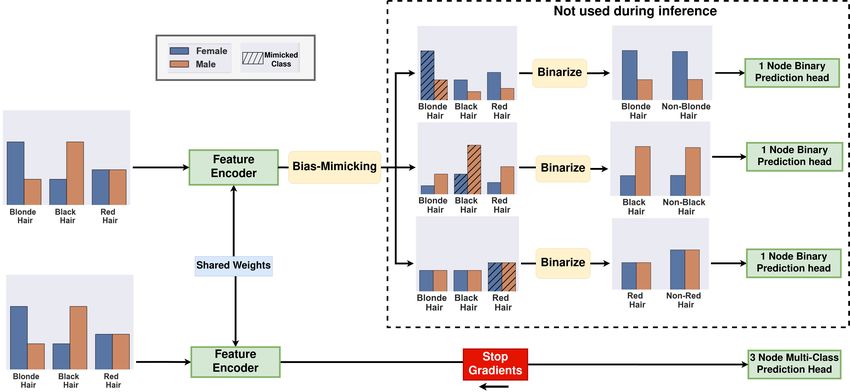
Dataset resampling methods, popular within the class              parisons used in prior work [12, 33, 35]. Despite their short-
imbalance literature [3, 8, 13, 29], present a simpler and            comings, we show that Undersampling and Upweighting
cheaper alternative. They do not require hyperparameter               are surprisingly competitive on many bias mitigation bench-
tuning or extra model parameters. Therefore, they are faster          marks. Therefore, this emphasizes these methods’ impor-
to train. Moreover, as illustrated in Figure 1(a), they can be        tance as an inexpensive first choice for mitigating bias.
extended to Bias Mitigation by considering the imbalance              However, in cases where these methods are ineffective, Bias
within the dataset subgroups rather than classes. Most com-           Mimicking bridges the performance gap and achieves com-
mon of these methods are Undersampling [3, 13, 29] and                parable performance to nonsampling methods. Finally, we
Oversampling [35]. They mitigate class imbalance by alter-            thoroughly analyze our approach’s behavior through two
ing the dataset distribution through dropping/repeating sam-          experiments. First, we verify the importance of each dc to
ples, respectively. Another similar solution is Upweight-             the model’s predictive performance in Section 4.2. Second,
ing [4,30], which levels each sample contribution to the loss         we investigate our method’s sensitivity to the mimicking
function by appropriately weighting its loss value. How-              condition in Section 4.3. Both experiments showcase the
ever, these methods suffer from significant shortcomings.             importance of our design in mitigating bias.
For example, Undersampling drops a significant portion of                Our contributions can be summarized as:
the dataset per epoch, which could harm the models’ predic-           • We show that simple sampling methods can be compet-
tive capacity. Moreover, Upweighting can be unstable when               itive on some benchmarks when compared to non sam-
used with stochastic gradient descent [2]. Finally, models              pling state-of-the-art approaches.
trained with Oversampling, as shown by [35], are likely to            • We introduce a novel resampling method: Bias Mimick-
overfit due to being exposed to repetitive sample copies.               ing that bridges the performance gap between sampling
    To address these problems, we propose Bias Mimick-                  and nonsampling methods; it improves the average under-
ing (BM): a class-conditioned sampling method that mit-                 represented subgroups accuracy by > 3% compared to
igates the shortcomings of prior work. As shown in Fig-                 other sampling methods.
ure 1(b), given a dataset D with a set of three classes C,            • We conduct an extensive empirical analysis of Bias Mim-
BM subsamples D and produces three different variants.                  icking that details the method’s sensitivity to the Mimick-
Each variant, dc ⊂ D retains every sample from class c                  ing condition and uncovers insights about its behavior.
while subsampling each c′ ̸= c such that c′ bias distribu-
tion, i.e. Pdc (B|Y = c′ ), mimics that of c. For example,            2. Related Work
observe dBlonde Hair in Figure 1(b) bottom left. Note how the         Documenting Spurious Correlations. Bias in Machine
bias distribution of class ”Blonde Hair” remains the same             Learning can manifest in many ways. Examples include
while the bias distributions of ”Black Hair” and ”Red Hair”           class imbalance [13], historical human biases [32], evalu-
are subsampled such that they mimic the bias distribution             ation bias [8], and more. For a full review, we refer the
of ”Blonde Hair”. This mimicking process decorrelates Y               reader to [23]. In our work, we are interested in model bias
from B since Y and B are now statistically independent as             that arises from spurious correlations. A spurious correla-
we prove in Section 3.1.                                              tion results from underrepresenting a certain group of sam-
    The strength of our method lies in the fact that dc re-           ples (e.g. samples with the color red) within a certain class
tains class c samples while at the same time ensuring                 (e.g. planes). This leads the model to learn the false rela-
Pdc (Y |B) = Pdc (Y ) in each dc . Using this result, we intro-       tionship between the class and the over-represented group.
duce a novel training procedure that uses each distribution           Prior work has documented several occurrences of this bias.
separately to train the model. Consequently, the model is             For example, [10,21,31,36] showed that state-of-the-art ob-
exposed to the entirety of D since each dc retains class c            ject recognition models are biased toward backgrounds or
samples. Refer to Section 3.1 for further details. Note how           textures associated with the object class. [1, 7] showed sim-
our method is fundamentally different from Undersampling.             ilar spurious correlations in VQA. [38] noted concerning
While Undersampling also ensures statistical independence             correlations between captions and attributes like skin color
on the dataset level, it subsamples every subgroup. There-            in Image-Captioning datasets. Beyond uncovering these
fore, the training distribution per epoch is a smaller portion        correlations within datasets, prior work like [12, 35] intro-
of the total dataset D. Moreover, our method is also differ-          duced synthetic bias datasets where they systematically as-
ent from Oversampling since each dc does not repeat sam-              sessed bias effect on model performance. Most recently,
ples. Thus we reduce the risk of overfitting.                         [24] demonstrates how biases toward gender are ubiquitous
    In addition to proposing Bias Mimicking, another con-             in the COCO and OpenImages datasets. As the authors
tribution of our work is providing an extensive analysis              demonstrate, these artifacts vary from low-level information
of sampling methods for bias mitigation. We found many                (e.g., the mean value of the color channels) to the higher
sampling-based methods were notably missing in the com-               level (e.g., pose and location of people).

                                                                  2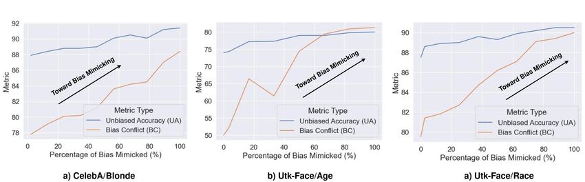
Figure 2. Given a dataset D with three classes, Bias Mimicking subsamples D and produces three different distributions. Each distribution
dc ⊂ D retains class c samples while subsampling each c′ ̸= c to ensure the bias distribution of c, i.e. Pdc (B|Y = c) is mimicked
in each c′ . To train an image classification model on the resulting distributions, we binarize each and feed it through a dedicated binary
prediction head. Alternatively, we could dedicate a multi-class prediction head for each distribution. However, this alternative will introduce
significantly more parameters. Put together, the binary prediction heads are equivalent #parameters wise to a model that uses one multi-
class prediction head. To perform inference, we can not use the scores from the binary predictors because they may not be calibrated with
respect to each other. Therefore, we train a multi-class prediction head using the debiased feature encoder from Bias Mimicking and freeze
the gradient from flowing back to ensure the bias is not relearned.

Nonsampling solutions. In response to the documenta-                      However, as noted in the introduction, some of these meth-
tion of dataset spurious correlations, several model-focused              ods have been missing in recent visual Bias Mitigation
methods have been proposed [12, 15, 26, 28, 33, 35]. For ex-              Benchmarks [12, 33, 35]. Thus, we review these meth-
ample, [33] presents a metric learning-based method where                 ods and describe their shortcomings in Section 3.2. Al-
model feature space is regularized against learning harm-                 ternatively, other efforts attempt to fix the dataset distribu-
ful correlations. [35] surveys several existing methods, such             tion by introducing new samples. Examples include [19],
as adversarial training, that randomize the relationship be-              where they introduce a new dataset for face recognition bal-
tween target classes and bias groups in the feature space.                anced among several race groups, and [25], where they used
They also present a new approach, domain independence,                    GANs to generate training data that balance the sizes of
where different prediction heads are allocated for each sub-              dataset subgroups. While our work is a dataset-based ap-
group. [28] presents GroupDRO (Distributionally Robust                    proach, it differs from these efforts as it does not generate or
Neural Networks for Group Shifts), a regularization pro-                  introduce new samples. Finally, also related to our work are
cedure that adapts the model optimization according to                    sampling methods like REPAIR [20], where a function is
the worst-performing group. Most recently, [12] extended                  learned to prioritize specific samples and, thus, learn more
contrastive learning frameworks on self-supervised learn-                 robust representations.
ing [6, 9, 14] to mitigate bias. Our work complements these
efforts by introducing a hyperparameter-free sampling al-                 3. Sampling For Bias Mitigation
gorithm that bridges the performance gap between nonsam-
pling and sampling methods.                                                  In visual bias mitigation, the goal is to train a model
                                                                          that does not rely on spurious signals in the images when
Dataset based solutions. In addition to model-based ap-                   making predictions (e.g. not using gender signal when pre-
proaches, we can mitigate spurious correlations by fixing                 dicting hair color). Formally, assume we have a dataset
the training dataset distribution. Examples include Over-                 of image/target-classes/bias-group triplets (X, Y, B) where
sampling minority classes, Undersampling majority ones,                   the images X contain components denoted as Xb that de-
and weighting the loss value of different samples to equalize             termine their bias group memberships B. Furthermore, let
the contribution of dataset subgroups. These approaches are               C represents the set of possible target-classes, and S rep-
popular within the class imbalance literature [3, 8, 13, 29].             resents the set of possible bias groups. We characterise

                                                                      3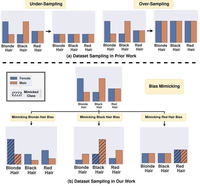
a model behavior as biased when the model uses the bi-              proposition above is a simple application of the law of total
ased image signal, i.e. Xb , to predict Y . This behavior           probability. Given s ∈ S, then
might arise when a target class c ∈ C (e.g. blonde hair)
is over-represented by images that belong to one bias group                 P_D(B = s) = \sum _{c \in C} P_D(B = s | Y = c) P_D(Y = c)                                                                                                                                                                                          (1)
s ∈ S (e.g. female) rather than distributed equally among
the dataset bias groups. In other words, there exists s ∈ B
                                                          1         Given our assumption of bias mimicking, i.e. PD (B =
for certain class c ∈ C such that PD (B = s|Y = c) >> |S|
                                                                    s|Y = i) = PD (B = s|Y = j) ∀i, j ∈ C, then we
where |S| denotes the number of bias groups. For example,           can rewrite (1) ∀c ∈ C as:
if most blonde hair samples were female, the model might
use the image components corresponding to gender in mak-                 P_D(B = s) & = P_D(B = s | Y = c) \sum _{c^{\prime } \in C} P_D(Y = c^{\prime })\\ &= P_D(B = s | Y = c)
ing predictions rather than solely relying on hair color.
    Our work addresses methods that fix spurious correla-                                                                                                                                                                                                                                                                       (3)
tions by ensuring statistical independence between Y and
B on the dataset level, i.e. PD (Y |B) = PD (Y ). In that           From here, using Bayesian probability and the result from
spirit, we introduce a new sampling method: Bias Mimick-            (3), we can write, ∀c ∈ C:
ing in Section 3.1. However, as we note in our introduction,
some popular sampling solutions in class imbalance litera-             P_D(Y=c | B=s) &= \frac {P_D(B=s | Y=c)P_D(Y=c)}{P_D(B=s)} \\ &= \frac {P_D(B=s)P_D(Y=c)}{P_D(B=s)} \\ &= P_D(Y=c)
ture that could also be applied to Bias Mitigation (e.g. Un-
dersampling, Upweighting) are missing from benchmarks
used in prior work. Therefore, we briefly review the missing
methods in Section 3.2 and describe how Bias Mimicking                                                                                                                                                                                                                                                                          (6)
addresses their shortcomings.
                                                                    We use this result to motivate a novel way of subsampling
3.1. Bias Mimicking
                                                                    the input distribution that ensures the model is exposed to
   The goal of our method is to prevent the model from us-          every sample in the dataset. To that end, for every class
ing the biased signal in the images, denoted as Xb , in mak-        c ∈ C, we produce a subsampled version of the dataset
ing predictions Ŷ . Our approach is inspired by Sampling           D denoted as dc ⊂ D. Each dc preserves its respective
methods, which mitigate this problem by enforcing statisti-         class c samples, i.e., all the samples from class c remain
cal Independence between the target labels Y and the bias           in dc , while subsampling every c′ ̸= c such that the bias
groups B in the dataset, i.e., PD (Y |B) = PD (Y ). How-            distribution in class c; i.e. Pdc (B|Y = c), is mimicked in
ever, simple sampling methods like Oversampling, Under-             each c′ . Formally:
sampling, and Upweighting need to be improved as we dis-
cuss in the introduction. We address these shortcomings in              \label {eq:biasmimick} P_{d_c}(B=s | Y = c) = P_{d_c}(B = s | Y = c^{\prime }) \quad \forall s \in S.  (7)
our proposed sampling algorithm: Bias Mimicking.
                                                                       Indeed, as Figure 2 illustrates, a dataset of three classes
Mimicking Distributions The key to our algorithm is the             will be subsampled in three different ways. In each ver-
observation that if the distribution of bias groups with re-        sion, a class bias is mimicked across the other classes. Note
spect to a class c; i.e., PD (B|Y = c), was the same across         that there is not unique solution for mimicking distributions.
every c ∈ C, then B is statistically independent from Y . For       However, we can constrain the mimicking process by en-
example, consider each resulting distribution from our Bias         suring that we retain the most number of samples in each
Mimicking process in Figure 2. Note how in each resulting           subsampled c′ ̸= c. We enforce this constraint naturally
distribution, the distribution of bias group ”Gender” is the        through a linear program. Denote the number of samples
                                                                                                                                 ′
same across every class ”Hair Color” which ensures statis-          that belong to class c′ as well as the bias group s as lsc .
                                                                                                        ′
tical independence between ”Gender” and ”Hair Color” on             Then we seek to optimize each lsc as follows:
the dataset level. Formally:
Proposition 1. Given dataset D, target classes set C, bias                                        \notag \max \quad &\sum _{s} l^{c^{\prime }}_s \\ \text {s.t.\quad } & l^{c^{\prime }}_s \leq |D_{c^{\prime }, s}| & & s \in S\\ & \frac {l^{c^{\prime }}_s}{\sum _{s} l^{c^{\prime }}_s } = P_{D}(B=s | Y = c) & & s \in S
groups set S, target labels Y , bias groups labels B, and
bias group s ∈ S if PD (B = s|Y = i) = PD (B =
s|Y = j) ∀i, j ∈ C, then PD (Y = c|B = s) = PD (Y =                 (P.1)
c) ∀c ∈ C.                                                                                                                                                                                                                                                                                                                      (9)
   Note that ensuring this proposition holds for every s ∈
S (i.e. the distribution of PD (B|Y = c) is the same for            where |Dc,s | represents the number of samples that belong
each c ∈ C) implies that PD (Y |B) = PD (Y ). Proving the           to both class c and bias group s. This linear program returns

                                                                4
the distribution with most number of retained samples while distribution of classes. Thus, they can be extended to
ensuring that the mimicking condition holds. Bias Mitigation by balancing groupings of classes and bias
Training with Bias Mimicking We use every resulting groups (e.g. group male-black hair). Prior work in Visual
dc ⊂ D to train the model. However, we train our model Bias Mitigation has explored one of these solutions: Over-
such that it sees each dc through a different prediction head sampling [35]. However, other methods like Undersam-
to ensure that the loss function does not take in gradients pling [3, 13, 29] and Upweighting [4, 30] are popular alter-
of repetitive copies, thus risking overfitting. A naive way natives to Oversampling. Both methods, however, have not
of achieving this is to dedicate a multi-class prediction head been benchmarked in recent Visual Bias Mitigation work
for each dc . However, this choice introduces (|C| − 1) addi- [12, 33]. We review these sampling solutions below and
tional prediction heads compared to a model that uses only note how Bias Mimicking addresses their shortcomings.
one. To avoid this, we binarise each dc and then use it to Undersampling drops samples from the majority classes
train a one-vs-all binary classifier BPc for each c. Each until all classes are balanced. We can extend this solution
head is trained on image-target pairs from its correspond- to Bias Mitigation by dropping samples to balance dataset
ing distribution dc as Figure 2 demonstrates. Note that each subgroups where a subgroup includes every sample that
binary predictor is simply one output node. Therefore, the shares a class c and bias group s, i.e., Dc,s = {(x, y, s) ∈
binary predictors introduce no extra parameters compared D s.t Y = c, B = s}. Then, we drop samples from each
to a multi-class head. Finally, given our setup, a prediction subgroup until each has a size equal to min |Dc,s |. Thus,
c,s
head might see only a small number of samples at certain in each epoch, the number of samples the model can see is
iterations. We mitigate this problem by accumulating the limited by the size of the smallest subgroup. While we can
gradients of each prediction head across iterations and only mitigate this problem by resampling the distribution each
backpropagating them once the classifier batch is full. epoch, the model, nevertheless, has to be exposed to re-
Inference with Bias Mimicking Using the binary classi- peated copies of the minority subgroup every time it sees
fiers during inference is challenging since each was trained new samples from the majority subgroups, which may com-
on different distributions, and their scores, therefore, may promise the predictive capacity of our model, as our exper-
not be calibrated. However, Bias Mimicking minimizes imental results demonstrate. Bias Mimcking addresses this
the correlation between Y and B within the feature space. shortcoming by using each dc ⊂ D, thus ensuring that the
Thus, we exploit this fact by training a multi-class predic- model is exposed to all of D every epoch.
tion head over the feature space using the original dataset Oversampling solves class imbalance by repeating copies
distribution. However, this distribution is biased; therefore, of samples to balance the number of samples in each
we stop gradients from flowing into the model backbone class. Similarly to Undersampling, it can also be easily
when training that layer to ensure that the bias is not learned extended to Bias Mitigation by balancing samples across
again in the feature space, as Figure 2 demonstrates. sensitive subgroups. In our implementation, we determine
Cost Analysis Unlike prior work [12, 33], bias mimicking the maximum size subgroup (i.e. max |Dc,s | where Dc,s =
involves no extra hyper-parameters. The debiasing is auto- c,s
matic by definition. This means that the hyper-parameter {(x, y, s) ∈ D s.t Y = c, B = s}) and then repeat samples
search space of our model is smaller than other bias mit- accordingly in every other subgroup. However, repeating
igation methods like [12, 28]. Consequently, our method samples as [35] shows, cause overfitting with overparame-
is cheaper and more likely to generalize to more datasets terized models like neural nets. Bias Mimicking addresses
as we show in Section 4.1. Moreover, note that the addi- this problem by not repeating samples in each subsampled
tional input distributions dc do not result in longer epochs; version of the dataset dc ⊂ D.
we make one pass only over each sample x during an epoch Upweighting Upweighting levels the contribution of dif-
and apply its contribution to the relevant BPy (s). Our only ferent samples to the loss function by multiplying its loss
additional cost is solving the linear program P.1 and train- value by the inverse of the sample’s class frequency. We can
ing the multi-class prediction head. However, training the extend this process to Bias Mitigation by simply consider-
linear layer is simple, fast, and cheap since it is only one ing subgroups instead of classes. More concretely, assume
linear layer. Moreover, the linear program is solved through model weights w, sample x, class c, bias s, and subgroup
modern and efficient implementations that take seconds and Dc,s = {(x, y, s) ∈ D s.t Y = c, B = s}, then the model
only needs to be done once for each dataset. optimizes:
3.2. Simple Sampling Methods L = E_{x, c, s} \Big [\frac {1}{p_D(x\in D_{c, s})} l(x, c ; w)\Big ]
As discussed in the introduction, the class imbalance lit-
erature is rich with dataset sampling solutions [3,5,8,13,29]. A key shortcoming of Upweighting is its instability
These solutions address class imbalance by balancing the when used with stochastic gradient descent [2]. Indeed,
5Non Sampling Methods Sampling Methods
Vanilla Adv [11] G-DRO [27] DI [35] BC+BB [12] OS [35] UW [4] US [13] BM (ours)
UTK-Face UA 72.8±0.2 70.2±0.1 74.2±0.9 75.5±1.1 78.9±0.5 76.6±0.3 78.8±1.2 78.2±1.0 79.7±0.4
Age BC 47.1±0.3 44.1±1.2 75.9±2.9 58.8±3.0 71.4±2.9 58.1±1.2 77.2±3.8 69.8±6.8 79.1±2.3
UTK-Face UA 88.4±0.2 86.1±0.5 90.8±0.3 90.7±0.1 91.4±0.2 91.3±0.6 89.7±0.6 90.8±0.2 90.8±0.2
Race BC 80.8±0.3 77.1±1.3 90.2±0.3 90.9±0.4 90.6±0.5 90.0±0.7 89.2±0.4 89.3±0.6 90.7±0.5
CelebA UA 82.4±1.3 82.4±1.3 90.4±0.4 90.9±0.5 90.4±0.2 88.1±0.5 91.6±0.3 91.1±0.2 90.8±0.4
Blonde BC 66.3±2.8 66.3±2.8 89.4±0.5 86.1±0.8 86.5±0.5 80.1±1.2 88.3±0.5 88.5±1.8 87.1±0.6
UA 88.7±0.1 81.8±2.5 89.1±0.2 92.1±0.0 90.9±0.2 87.8±0.2 86.5±0.5 88.2±0.4 91.6±0.1
CIFAR-S
BC 82.8±0.1 72.0±0.2 88.0±0.2 91.9±0.2 89.5±0.7 82.5±0.3 80.0±0.7 83.7±1.2 91.1±0.1
UA 83.0±0.4 80.1±1.1 86.1±0.4 87.3±0.4 87.9±0.3 85.9±0.4 86.6±0.6 87.0±0.4 88.2±0.3
Average
BC 69.2±0.8 64.8±1.4 85.8±1.0 81.9±1.1 84.5±1.1 77.6±0.8 83.6±1.3 82.8±2.6 87.0±0.9
Table 1. Results compare methods Adversarial training (Adv) [16], GroupDRO (G-DRO) [27], Domain Independence DI [35], Bias
Contrastive and Bias-Contrastive and Bias-Balanced Learning (BC+BB) [12], Undersampling (US) [13], Upweighting (UW) [4], and Bias
Mimicking (BM, ours), on the CelebA, UTK-face, and CIFAR-S dataset. Methods are evaluated using Unbiased Accuracy [12] (UA),
Bias-conflict [12] (BC). Given the methods’ grouping: Sampling/Non Sampling, the Underlined numbers indicate the best method per
group on each dataset while bolded numbers indicate the best method per group on average. See Section 4.1 for discussion.
we demonstrate this problem in our experiments in Sec- that prior work [12, 33] used the HeavyMakeUp attribute
tion 4 where Upweighting does not work well on some in their CelebA benchmark. However, during our experi-
datasets. Bias Mimicking addresses this problem by not us- ments, we found serious problems with the benchmark. Re-
ing weights to scale the loss function. fer to the supplementary for model details. Therefore, we
skip this benchmark in our work. For UTKFace, we fol-
4. Experiments low [12] and do the binary classification with Race/Age as
the sensitive attribute and Gender as the target attribute. We
We report our method performance on four total bench- use [12] split for both tasks. With regard to CIFAR-S, The
marks: three binary and one multi-class classification benchmark synthetically introduces bias into the CIFAR-10
benchmark in Section 4.1. In addition to reporting our dataset [18] by converting a subsample of images from each
method results, we include vanilla sampling methods, target class to a gray-scale. We use [35] version where half
namely Undersampling, Upweighting, and Oversampling, of the classes are biased toward color and the other half is
which, as noted in our introduction, have been missing biased toward gray where the dominant sensitive group in
from recent Bias Mitigation work [12,28,35]. Furthermore, each target represents 95% of the samples.
we report the averaged performance overall benchmarks to Metrics Using Average accuracy on each sample is a mis-
highlight methods that generalize well to all datasets. We leading metric. This is because the test set could be biased
then follow up our results with two main experiments that toward some subgroups more than others. Therefore, the
analyze our method’s behavior. The first experiment in Sec- metric does not reflect how the model performs on all sub-
tion 4.2 analyzes the contribution of each subsampled ver- groups. Methods, therefore, are evaluated in terms of Unbi-
sion of the dataset: dc to model performance. The second ased Accuracy [12], which computes the accuracy of each
experiment in Section 4.3 is a sensitivity analysis of our subgroup separately and then returns the mean of accura-
method to the mimicking condition. cies, and Bias-Conflict [12], which measures the accuracy
on the minority subgroups.
4.1. Main Results
Baselines We report several baselines from prior work.
Datasets We report performance on three main datasets: First, we report ”Bias-Contrastive and Bias-Balanced
CelebA dataset [22] UTKFace dataset [37] and CIFAR-S Learning” (BC + BB) [12], which uses a contrastive
benchmark [35]. Following prior work [12, 33], we train learning framework to mitigate bias. Second, domain-
a binary classification model using CelebA where Blond- independent (DI) [35] uses an additional prediction head
Hair is a target attribute and Gender is a bias attribute. We for each bias group. GroupDRO [27] which optimizes a
use [12] split where they amplify the bias of Gender. Note worst-group training loss combined with group-balanced
6UAc1 UAc2 UA UAc1 UAc2 UA UAc1 UAc2 UA
(dc1 ) 82.5 74.2 78.4±0.5 (dc1 ) 90.7 85.1 87.9±0.5 (dc1 ) 91.5 90.3 90.9±0.1
(dc2 ) 73.1 67.9 70.5±2.3 (dc2 ) 84.8 91.5 88.1±0.6 (dc2 ) 82.2 96.5 89.3±0.1
(dc1 , dc2 ) 84.4 75.3 79.8±0.9 (dc1 , dc2 ) 90.5 91.1 90.8±0.2 (dc1 , dc2 ) 88.1 94.2 90.8±0.4
(a) Utk-Face/Age (b) Utk-Face/Race (c) CelebaA/Blonde
Table 2. We investigate the effect of each resampled version of the dataset dc on model performance using the binary classification tasks
outlined in Section 4.1. Thus, Bias Mimicking results in two subsampled distributions dc1 and dc2 . We then train three different models:
1) a model trained on only dc1 , 2) a model trained on only dc2 and a model trained on both (default choice for Bias Mimicking). We use
the Unbiased Accuracy metric (UA). Furthermore, we report UA on class 1: UA1 and class 2: UA2 separately by averaging the accuracy
over the class’s relevant subgroups. Refer to section 4.2 for discussion.
resampling. Adversarial Learning (Adv) w/ uniform con- a strong baseline. We encourage future work, therefore, to
fusion [11] introduces an adversarial loss that seeks to ran- add these sampling methods as part of their baselines.
domize the model’s feature representation of Y and B. With respect to non-sampling methods, our method
Furthermore, we expand the benchmark by reporting the (BM) maintains strong comparable performance. This
performance of sampling methods outlined in Section 3. strong performance comes with no additional loss functions
Note that since Undersampling and Oversampling result in or any model modification which limits the hyper-parameter
smaller/larger distributions per epoch than other methods, space and implementation complexity of our method com-
we adjust their number of training epochs such that the pared to non-sampling methods. For example, BC+BB [12]
model sees the same number of data batches throughout the requires a scalar parameter to optimize an additional loss. It
training process as other methods in our experiment. Re- also requires choosing a set of augmentation functions for
fer to the Supplementary for further details. Finally, all re- its contrastive learning paradigm, which must be tuned ac-
ported methods are compared to a ”vanilla” model trained cording to the dataset. GroupDRO [28], on the other hand,
on the original dataset distribution with a Cross-Entropy requires careful L2 regularization as well as tuning their
loss. All baselines are trained using the same encoder. Re- ”group adjustment” hyper parameter. As a result, BM is
fer to the Supplementary for further details. faster and cheaper to train.
Results in Table 1 demonstrates how BM is the most ro-
bust sampling method. It achieves strong performance on 4.2. The Effect of Each dc on Model Performance
every dataset, unlike other sampling methods. For ex-
ample, Undersampling while performing well on CelebA For each class, c ∈ C, Bias Mimicking returns a subsam-
(likely because the task of predicting hair color is easy), pled version of the dataset dc ⊂ D where class c samples
performs considerably worse on every other dataset. More- are preserved, and the bias of c is mimicked in the other
over, Oversampling, performs consistently worse than our classes. In this section, we investigate the effect of each dc
method. This aligns with [35] observation that neural nets on performance. We use the binary classification tasks in
tend to overfit when trained on oversampled distributions. Section 4.1. For each task, thus, we have two versions of
Finally, while Upweighting maintains strong performance the dataset dc1 , dc2 where c1 is the first class and c2 is the
on CelebA and UTK-Face, it falls behind on CIFAR-S. This second. We compare three different models performances:
is because the method struggled to optimize, a property of model (1) trained on only dc1 , model (2) trained on only
Upweighting that has been noted and discussed in [2]. BM, dc2 , and finally, model (3) trained on both (dc1 , dc2 ). The
consequently, improves over Upweighting on CIFAR-S by last version is the one used by our method. We use the
over %10 on the Bias Conflict metric. Unbiased Accuracy Metric (UA). We also break down the
While our method is the only sampling method that metric into two versions: UA1 where accuracy is averaged
shows consistently strong performance, vanilla sampling over class 1 subgroups, and UA2 where accuracy is aver-
methods are surprisingly effective on some datasets. For aged over class 2 subgroups. Observe the results in Table
example, Upweighting is effective on UTK-Face and 2. Overall, the model trained on (dc1 ) performs better at
CelebA, especially when compared to non-sampling meth- predicting c1 but worse at predicting c2 . We note the same
ods. Moreover, Undersampling similarly is more effective trend with the model trained on (dc2 ) but in reverse. This
than non-sampling methods on CelebA. This is evidence disparity in performance harms the average Unbiased Accu-
that when enough data is available and the task is ”easy” racy (UA). However, a model trained on (dc1 , dc2 ) balances
enough, then simple Undersampling is effective. These re- both accuracies and achieves the best total Unbiased Accu-
sults are important because they show how simply fixing racy (UA). These results emphasize the importance of each
the dataset distribution through sampling methods could be dc for good performance.
7Figure 3. Model Sensitivity to Bias Mimicking We test our method’s sensitivity to the Bias Mimicking condition in Equation 7. To that
end, we simulate multiple scenarios where we mimic the bias by x% ∈ {0, 100} (x-axis) such that 0% represents no modification to the
distribution and 100% represents complete Bias Mimicking. We report results on the three binary classification benchmarks defined in
Section 4.1. Refer to Section 4.3 for further details and discussion.
4.3. Model Sensitivity to the Mimicking Condition that some are surprisingly effective on many datasets. How-
ever, on some others, their performance significantly lagged
In this section, we test the model sensitivity to the mim-
behind non sampling methods. Motivated by this observa-
icking condition outlined in Eq. 7. To that end, we con-
tion, we introduced a novel sampling method: Bias Mim-
sider the binary classification benchmarks in Section 4.1.
icking. The method retained the simplicity of sampling
These benchmarks have two classes, c1 and c2 , and two bias
methods while bridging the performance gap between sam-
groups, b1 and b2 . Each class is biased toward one of the
pling and non sampling methods. Furthermore, we exten-
bias groups. We vary the mimicking process according to a
sively analyzed the behavior of Bias Mimicking, which em-
percentage value where for value 0%, the resulting dc (s) are
phasized the importance of our design. We hope our new
the same as the original training distribution, and for value
method can reestablish sampling methods as a promising
x > 0%, dc (s) are subsampled from the main training dis-
direction for bias mitigation.
tribution such that the bias is mimicked by x%. Note how,
therefore, 100% represents the full mimicking process as Limitations And Future Work We demonstrated that
outlined in Eq. 7 whereas x = 50% mimicks the bias by dataset re-sampling methods are simple and effective tools
half. Formally, if c2 needs to mimick c1 and c1 is biased in mitigating bias. However, we recognize that the explored
toward b1 then bias scenarios in prior and our work are still limited. For
example, current studies only consider mutually exclusive
sensitive groups. Thus, a sample can belong to only one
P_{d_{c_1}}(B = b_1 | Y=c_2 ) = \frac {1}{2} P_{d_{c_1}}(B = b_1 | Y=c_1 ) sensitive group at a time. How does relaxing this assump-
tion, i.e. intersectionality, impact bias? Finally, the dataset
re-sampling methods presented in this work are effective
Observe the result in Figure 3. Note that as the percent-
at mitigating bias when enough samples from all dataset
age of bias Mimicked decreases, the BC and UA decrease
subgroups are available. However, it is unclear how these
as expected. This is because PD (Y |B) ̸= PD (Y ) following
methods could handle bias scenarios when one class is com-
proposition 1. More interestingly, note how the Bias Con-
pletely biased by one sensitive group. Moreover, sampling
flict (the accuracy over the minority subgroups) decreases
methods require full knowledge of the bias groups labels at
much faster. The best performance is achieved when x%
training time. Collecting annotations for these groups could
is indeed 100% and thus PD (Y |B) = PD (Y ). From this
be expensive. Future work could benefit from building more
analysis, we conclude that the Bias Mimicking condition is
robust models independently of bias groups labels.
critical for good performance.
Acknowledgements This material is based upon work
supported, in part, by DARPA under agreement number
5. Conclusion
HR00112020054 and the National Science Foundation, in-
In this paper, we observed that hyper-parameter-free cluding under Grant No. DBI-2134696. Any opinions, find-
sampling methods for bias mitigation like Undersampling ings, and conclusions or recommendations expressed in this
and Upweighting were missing from recent benchmarks. material are those of the author(s) and do not necessarily re-
Therefore, we benchmarked these methods and concluded flect the views of the supporting agencies.
8References [13] Nathalie Japkowicz and Shaju Stephen. The class imbal-
ance problem: A systematic study. Intelligent Data Analysis,
[1] Aishwarya Agrawal, Dhruv Batra, Devi Parikh, and Anirud- pages 429–449, 2002. 2, 3, 5, 6, 11, 12
dha Kembhavi. Don’t just assume; look and answer: [14] Prannay Khosla, Piotr Teterwak, Chen Wang, Aaron Sarna,
Overcoming priors for visual question answering. 2018 Yonglong Tian, Phillip Isola, Aaron Maschinot, Ce Liu,
IEEE/CVF Conference on Computer Vision and Pattern and Dilip Krishnan. Supervised contrastive learning. In
Recognition, pages 4971–4980, 2018. 2 H. Larochelle, M. Ranzato, R. Hadsell, M. F. Balcan, and
[2] Jing An, Lexing Ying, and Yuhua Zhu. Why resampling H. Lin, editors, Advances in Neural Information Process-
outperforms reweighting for correcting sampling bias with ing Systems, volume 33, pages 18661–18673. Curran Asso-
stochastic gradients. In 9th International Conference on ciates, Inc., 2020. 3
Learning Representations, ICLR 2021, Virtual Event, Aus- [15] Byungju Kim, Hyunwoo Kim, Kyungsu Kim, Sungjin Kim,
tria, May 3-7, 2021. OpenReview.net, 2021. 2, 5, 7 and Junmo Kim. Learning not to learn: Training deep neural
[3] Mateusz Buda, Atsuto Maki, and Maciej A. Mazurowski. A networks with biased data. In 2019 IEEE/CVF Conference
systematic study of the class imbalance problem in convo- on Computer Vision and Pattern Recognition (CVPR), pages
lutional neural networks. Neural Networks, 106:249–259, 9004–9012, 2019. 1, 3
2018. 2, 3, 5 [16] Byungju Kim, Hyunwoo Kim, Kyungsu Kim, Sungjin Kim,
[4] Jonathon Byrd and Zachary Lipton. What is the effect and Junmo Kim. Learning not to learn: Training deep neural
of importance weighting in deep learning? In Kamalika networks with biased data. In The IEEE Conference on Com-
Chaudhuri and Ruslan Salakhutdinov, editors, Proceedings puter Vision and Pattern Recognition (CVPR), June 2019. 6
of the 36th International Conference on Machine Learning, [17] Diederik Kingma and Jimmy Ba. Adam: A method for
volume 97 of Proceedings of Machine Learning Research, stochastic optimization. International Conference on Learn-
pages 872–881. PMLR, 09–15 Jun 2019. 2, 5, 6, 11 ing Representations, 12 2014. 12
[5] Nitesh Chawla, Kevin Bowyer, Lawrence Hall, and W. [18] Alex Krizhevsky. Learning multiple layers of features from
Kegelmeyer. Smote: Synthetic minority over-sampling tech- tiny images. University of Toronto, 05 2012. 6
nique. J. Artif. Intell. Res. (JAIR), 16:321–357, 06 2002. 5 [19] Kimmo Kärkkäinen and Jungseock Joo. Fairface: Face at-
tribute dataset for balanced race, gender, and age for bias
[6] Ting Chen, Simon Kornblith, Kevin Swersky, Mohammad
measurement and mitigation. In 2021 IEEE Winter Con-
Norouzi, and Geoffrey Hinton. Big self-supervised mod-
ference on Applications of Computer Vision (WACV), pages
els are strong semi-supervised learners. arXiv preprint
1547–1557, 2021. 3
arXiv:2006.10029, 2020. 3
[20] Yi Li and Nuno Vasconcelos. Repair: Removing representa-
[7] Christopher Clark, Mark Yatskar, and Luke Zettlemoyer.
tion bias by dataset resampling. 2019 IEEE/CVF Conference
Don’t take the easy way out: Ensemble based methods for
on Computer Vision and Pattern Recognition (CVPR), pages
avoiding known dataset biases. In Proceedings of the 2019
9564–9573, 2019. 3
Conference on Empirical Methods in Natural Language Pro-
[21] Yingwei Li, Qihang Yu, Mingxing Tan, Jieru Mei, Peng
cessing and the 9th International Joint Conference on Nat-
Tang, Wei Shen, Alan Yuille, and Cihang Xie. Shape-
ural Language Processing (EMNLP-IJCNLP), pages 4069–
texture debiased neural network training. arXiv preprint
4082, Hong Kong, China, Nov. 2019. Association for Com-
arXiv:2010.05981, 2020. 2
putational Linguistics. 2
[22] Ziwei Liu, Ping Luo, Xiaogang Wang, and Xiaoou Tang.
[8] Joy Buolamwini et al. Gender shades: Intersectional accu- Deep learning face attributes in the wild. In ICCV, 2015.
racy disparities in commercial gender classification. In ACM 6, 10, 11, 12
FAccT, 2018. 2, 3, 5
[23] Ninareh Mehrabi, Fred Morstatter, Nripsuta Saxena, Kristina
[9] Kaiming He, Haoqi Fan, Yuxin Wu, Saining Xie, and Ross Lerman, and Aram Galstyan. A survey on bias and fairness
Girshick. Momentum contrast for unsupervised visual repre- in machine learning. ACM Comput. Surv., 54(6), jul 2021. 2
sentation learning. In 2020 IEEE/CVF Conference on Com- [24] Nicole Meister, Dora Zhao, Angelina Wang, Vikram V. Ra-
puter Vision and Pattern Recognition (CVPR), pages 9726– maswamy, Ruth C. Fong, and Olga Russakovsky. Gender
9735, 2020. 3 artifacts in visual datasets. ArXiv, abs/2206.09191, 2022. 2
[10] Dan Hendrycks, Kevin Zhao, Steven Basart, Jacob Stein- [25] Vikram V. Ramaswamy, Sunnie S. Y. Kim, and Olga Rus-
hardt, and Dawn Song. Natural adversarial examples. CVPR, sakovsky. Fair attribute classification through latent space
2021. 2 de-biasing. CoRR, abs/2012.01469, 2020. 3
[11] Judy Hoffman, Eric Tzeng, Trevor Darrell, and Kate Saenko. [26] Hee Jung Ryu, Margaret Mitchell, and Hartwig Adam. Im-
Simultaneous deep transfer across domains and tasks. 2015 proving smiling detection with race and gender diversity.
IEEE International Conference on Computer Vision (ICCV), CoRR, abs/1712.00193, 2017. 1, 3
pages 4068–4076, 2015. 6, 7, 11 [27] Shiori Sagawa, Pang Wei Koh, Tatsunori B. Hashimoto, and
[12] Youngkyu Hong and Eunho Yang. Unbiased classifica- Percy Liang. Distributionally robust neural networks. In
tion through bias-contrastive and bias-balanced learning. In ICLR, 2020. 1, 6, 11, 12
Thirty-Fifth Conference on Neural Information Processing [28] Shiori Sagawa, Pang Wei Koh, Tatsunori B Hashimoto, and
Systems, 2021. 1, 2, 3, 5, 6, 7, 10, 11, 12 Percy Liang. Distributionally robust neural networks for
9group shifts: On the importance of regularization for worst- BM BM+US BM+UW BM+OS
case generalization. In International Conference on Learn-
ing Representations (ICLR), 2020. 3, 5, 6, 7 UTK-Face UA 79.7±0.4 79.2±1.0 79.9±0.2 79.3±0.2
[29] Shiori Sagawa, Aditi Raghunathan, Pang Wei Koh, and Age BC 79.1±2.3 77.6±0.9 77.5±1.7 78.7±1.6
Percy Liang. An investigation of why overparameteriza-
tion exacerbates spurious correlations. In Hal Daumé III UTK-Face UA 90.8±0.2 90.9±0.5 91.1±0.2 90.7±0.4
and Aarti Singh, editors, Proceedings of the 37th Interna- Race BC 90.7±0.5 91.1±0.3 91.6±0.1 90.9±0.5
tional Conference on Machine Learning, volume 119 of Pro-
ceedings of Machine Learning Research, pages 8346–8356. CelebA UA 90.8±0.4 91.1±0.2 91.1±0.4 91.1±0.1
PMLR, 13–18 Jul 2020. 2, 3, 5
Blonde BC 87.1±0.6 87.9±0.3 87.9±0.7 87.7±0.4
[30] Hidetoshi Shimodaira. Improving predictive inference un-
der covariate shift by weighting the log-likelihood function. CIFAR-S UA 91.6±0.1 91.7±0.1 91.8±0.0 91.6±0.2
Journal of Statistical Planning and Inference, 90:227–244, BC 91.1±0.1 91.2±0.2 91.4±0.2 91.2±0.2
10 2000. 2, 5
[31] Krishna Kumar Singh, Dhruv Mahajan, Kristen Grauman,
Table 3. Sampling for multi-class prediction head compare the
Yong Jae Lee, Matt Feiszli, and Deepti Ghadiyaram. Don’t
effects of using different sampling methods to train the multi-class
judge an object by its context: Learning to overcome contex-
prediction in our proposed method: Bias Mimicking. We under-
tual bias. In CVPR, 2020. 2
line results where sampling methods make significant improve-
[32] Harini Suresh and John V. Guttag. A framework for un- ments. Refer to Section A for discussion.
derstanding unintended consequences of machine learning.
ArXiv, abs/1901.10002, 2019. 2 training is done, using the scores from each binary predictor
[33] Enzo Tartaglione, Carlo Alberto Barbano, and Marco for inference is challenging. This is because each predictor
Grangetto. End: Entangling and disentangling deep rep- is trained on a different distribution of the data, so the pre-
resentations for bias correction. In Proceedings of the
dictors are uncalibrated with respect to each other. There-
IEEE/CVF Conference on Computer Vision and Pattern
Recognition (CVPR), pages 13508–13517, June 2021. 1, 2,
fore, to perform inference, we train a multi-class prediction
3, 5, 6, 11 head using the learned feature representations and the origi-
[34] Angelina Wang, Arvind Narayanan, and Olga Russakovsky. nal dataset distribution. Moreover, we prevent the gradients
Vibe: A tool for measuring and mitigating bias in image from flowing into the feature space since the original distri-
datasets. CoRR, abs/2004.07999, 2020. 1 bution is biased. Note that we rely on the assumption that
[35] Zeyu Wang, Klint Qinami, Ioannis Karakozis, Kyle Genova, the correlation between the target labels and bias labels are
Prem Nair, Kenji Hata, and Olga Russakovsky. Towards minimized in the feature space, and thus the linear layer is
fairness in visual recognition: Effective strategies for bias unlikely to relearn the bias. During our experiments out-
mitigation. In Proceedings of the IEEE/CVF Conference on lined in Section 4, we note that this approach was sufficient
Computer Vision and Pattern Recognition (CVPR), 2020. 1, to obtain competitive results. This section explores whether
2, 3, 5, 6, 7, 11, 12 we can improve performance by using sampling methods to
[36] Kai Xiao, Logan Engstrom, Andrew Ilyas, and Aleksander train the linear layer. To that end, observe results in Table 3.
Madry. Noise or signal: The role of image backgrounds in We underline the rows where the sampling methods make
object recognition. ArXiv preprint arXiv:2006.09994, 2020.
improvements. We note that the sampling methods did not
2
improve performance for three of the four benchmarks in
[37] Zhifei Zhang, Yang Song, and Hairong Qi. Age progres-
our experiments. However, on CelebA, we note that the
sion/regression by conditional adversarial autoencoder. In
CVPR, 2017. 6, 12
sampling methods marginally improved performance. We
[38] Dora Zhao, Angelina Wang, and Olga Russakovsky. Under-
suspect this is because a small amount of the bias might
standing and evaluating racial biases in image captioning. In be relearned when training the multi-class prediction head
International Conference on Computer Vision (ICCV), 2021. since the input distribution remains biased.
1, 2
B. Heavy Makeup Benchmark
A. Sampling methods Impact on Multi-Class Prior work [12] uses the Heavy Makeup binary attribute
Classification Head prediction task from CelebA [22] as a benchmark for bias
mitigation, where Gender is the sensitive attribute. In this
Bias Mimicking produces a binary version dc of the experiment, Heavy Makeup’s attribute is biased toward the
dataset D for each class c. Each dc preserves class c sam- sensitive group: Female. We note that the notion of ”Heavy
ples while undersampling each c′ such that the bias within c′ Makeup” is quite subjective. The attribute labels may vary
mimics that of c. A debiased feature representation is then significantly according to cultural elements, lighting condi-
learned by training a binary classifier for each dc . When the tions, and camera pose considerations. Thus, we expect a
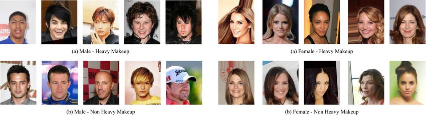
10Figure 4. Randomly sampled images from the four subgroups: Female-Heavy Makeup, Female-Non-Heavy Makeup, Male-Heavy Makeup,
and Male-Non-Heavy Makeup in CelebA dataset [22]. Note the that there is not a clearly differentiating signal for the attribute Heavy
Makeup. Refer to Section B for discussion.
Nonsampling Methods Sampling Methods
Vanilla Adv [11] G-DRO [27] DI [35] BC+BB [12] OS [35] UW [4] US [13] BM BM + OS
CelebA UA 90.9±0.1 90.7±0.2 93.2±0.1 92.0±0.1 92.4±0.1 92.4±0.3 92.8±0.0 92.6±0.1 92.7±0.1 92.7±0.1
Smiling BC 84.3±0.2 84.7±0.4 92.2±0.1 91.3±0.2 92.6±0.1 91.5±0.2 92.4±0.2 92.1±0.2 92.3±0.2 92.2±0.1
CelebA UA 86.3±0.7 87.1±0.3 88.5±0.2 86.7±0.7 87.7±0.1 87.6±0.3 88.5±0.1 88.4±0.2 87.6±0.7 88.5±0.1
Black Hair BC 82.7±0.6 83.4±0.5 88.3±0.4 86.6±1.2 86.6±0.3 85.6±0.6 88.0±0.2 87.3±0.1 87.8±1.3 88.5±0.7
UA 88.6±0.4 88.9±0.2 90.8±0.1 89.3±0.4 90.0±0.1 90.0±0.3 90.6±0.1 90.5±0.1 90.2±0.4 90.6±0.1
Average
BC 83.5±0.4 84.0±0.4 90.2±0.2 88.9±0.7 89.6±0.2 88.5±0.4 90.2±0.2 89.7±0.1 90.0±0.7 90.3±0.4
Table 4. Expanded benchmarks from the CelebA dataset [22]. Refer to Section C for discussion.
fair amount of label noise, i.e., inconsistency with label as- ing set, the small size of the under-represented group in the
signment. We document this problem in a Quantitative and test set, and its label noise, we conclude that results from
Qualitative analysis below. this benchmark will not be reliable and exclude it from our
experiments.
Quantitative Analysis: We randomly select a total of Qualitative Analysis: We sample random 5 images from
200 pairs of positive and negative images. We ensure the following subgroups: Female-Heavy Makeup, Female-
the samples are balanced among the four possible pair- Non-Heavy Makeup, Male-Heavy Makeup, and Male-Non-
ings, i.e., (Heavy Makeup-Male, Non Heavy Makeup- Heavy Makeup (Fig 4). It is clear from the Figure that there
Female), (Heavy Makeup-Female, Non Heavy Makeup- is no firm agreement about the definition of Heavy Makeup.
Male), (Heavy Makeup-Male, Non Heavy Makeup-Male),
(Heavy Makeup-Female, Non Heavy Makeup-Female). We C. Additional Benchmarks
asked three independent annotators to label which image in
the pair is wearing ”Heavy Makeup”. Then, we calculate In Section B, we note that the CelebA attribute Heavy-
the percentage of disagreement between the three annota- Makeup usually used in assessing model bias in prior work
tors and the ground truth labels in the dataset. We note that [12, 33] is a noisy attribute, i.e., labels are inconsistent.
32.3% ± 0.02 of the time, the annotators on average dis- Therefore, we choose not to use it in our experiments. Alter-
agreed with the ground truth. The noise is further amplified natively, we provide results on additional attributes where
when the test set used in [12] is examined. In particular, labels are more likely to be consistent. To that end, we
Male-Heavy Make up (an under-represented subgroup) only choose to classify the attributes: Smiling and Black Hair,
contains 9 testing samples. We could not visually determine where Gender is the bias variable. The original distribu-
whether 4 out of these 9 images fall under Heavy Makeup. tion of each attribute is not sufficiently biased with respect
Out of the 5 remaining images, 3 are of the same person to Gender to note any significant change in performance.
from different angles. Thus, given the noise in the train- Thus, we subsample each distribution to ensure that each
11Learning Weight Group US [13] OS [35] Other Methods
Rate Reg Adjustment
UTK-Face Age 400 7 20
UTK-Face Age 0.001 0.01 4 UTK-Face Race 120 10 20
UTK-Face Race 0.001 0.001 4
CelebA Blonde 170 4 10
CelebA Blonde 0.001 0.1 3 CelebA Black Hair 40 5 10
CelebA Smiling 0.0001 0.01 2 CelebA Smiling 30 5 10
CelebA Black Hair 0.0001 0.01 3
CIFAR-S 2000 100 200
CIFAR-S 0.01 0.01 5
Table 6. Number of Epochs used to train each method. Refer to
Table 5. Hyperparameters used for GroupDRO [27]. Refer to Sec- Section D for further discussion.
tion D for further discussion.
D. Model and Hyper-parameters Details
attribute is biased toward Gender. We provide the splits for We test bias Mimicking on six benchmarks. Three Bi-
the resulting distributions in the attached code base. Refer nary Classification tasks on CelebA [22], namely, Blonde,
for Table 4 for results. Black Hair, and Smiling, Two Binary Classification tasks on
Note that our method Bias Mimicking performance UTK-Face [37], namely Race and Age and one multi-class
marginally lags behind other methods when predicting task CIFAR-S. We provide further info below.
”Black Hair” attribute. However, when the multi-class pre- Optimization Following [12], we use ADAM [17] opti-
diction layer is trained with an oversampled distribution mizer with learning rate 0.0001 on CelebA and UTK-Face.
(BM + OS), then the gap is bridged. This is consistent with For CIFAR-S, following [35], we use SGD with learning
the observation in Table 3 where oversampling marginally rate 0.1. GroupDRO [27], however, has not been tuned
improves our method performance on CelebA. These obser- before on the benchmarks in our study. Even for CelebA
vations indicate that on some benchmarks, a small amount Blonde, the method was not tuned on the more challenging
of the bias might be relearned through the multi-class pre- split in this study. Therefore, we grid search the learning
diction head. To ensure that this bias is mitigated, it is suffi- rate/weight regularization/group adjustment and choose the
cient to oversample the input distribution. Moreover, since best over the validation set. Refer to Table 5 for our fi-
oversampling the input distribution does not change perfor- nal choices. With respect to BC+BB, the method was not
mance on other datasets as indicated in Table 3, we recom- benchmarked on CIFAR-S. Therefore, we run a grid search
mend that the input distribution for the multi-class predic- over the method’s hyperparameters and choose α = 1.0,
tion head is oversampled to ensure the best performance. γ = 10. Finally, as discussed in Section 4, UW struggles to
Overall, (BM + OS) performs comparably to sampling optimize over CIFAR-S with learning rate 0.1. Therefore,
and nonsampling methods. This is consistent with our re- we tune the learning rate and we find that 0.0001 to work
sults on CelebA dataset in Section 4 of the main paper the best over the validation set.
where we predict ”Blonde Hair”. More concretely, Un- Total Number of Epochs As noted in Section 4.1 in the
dersampling performs comparably and sometimes better paper, a model trained with Undersampling sees fewer it-
than nonsampling methods. This is reaffirming that pre- erations than baselines per epoch and a model trained with
dicting attributes on CelebA is relatively an easy task that Oversampling sees more iterations per epoch. Therefore,
dropping samples to balance subgroup distribution is suf- we adjust the number of epochs for both methods such that
ficient to mitigate bias. However, as discussed in Sec- the total number of iterations seen by the model is the same
tion 4 of the main paper, vanilla sampling methods (Un- across all methods tested in our experiments. Refer to Ta-
dersampling, Upweighting, Oversampling) perform poorly ble 6 for a breakdown of the total number of epochs used to
on some datasets. For example, as we note in Table 1 train each method.
in the main paper, Undersampling performs considerably
Augmentations: For all benchmarks, we augment the in-
worse than nonsampling methods on the Utk-Face dataset
put images with a horizental flip. BC+BB [12] uses extra
as well the CIFAR-S dataset. Moreover, Upweighting per-
augmentation functions. Refer to [12] for further details.
forms substantially worse on CIFAR-S. Finally, Oversam-
pling performs consistently worse on every benchmark. Splits: Note on CelebA, unlike [12], we use CelebA vali-
However, only our method, Bias Mimicking, manages to dation set for validation and test set for testing rather than
maintain competitive performance with respect to nonsam- using the validation set for testing and a split of the training
pling methods on all datasets. set for validation.
12You can also read