Converting a Static Macroscopic Model Into a Dynamic Activity-Based Model to Analyze Public Transport Demand in Berlin
←
→
Page content transcription
If your browser does not render page correctly, please read the page content below
Converting a Static Macroscopic Model Into a
Dynamic Activity-Based Model to Analyze
Public Transport Demand in Berlin

Andreas Neumann, Berlin Institute of Technology
Michael Balmer, Senozon AG
Marcel Rieser, Senozon AG

              Travel Behaviour Research: Current Foundations,
              Future Prospects

              13th International Conference on Travel Behaviour Research
              Toronto 15-20, July 2012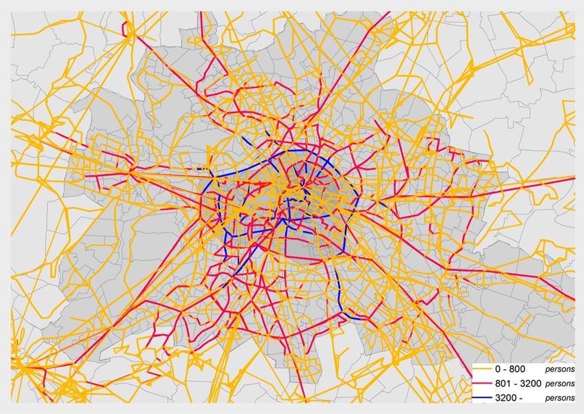
Converting a Static Macroscopic Model Into a Dynamic
Activity-Based Model to Analyze Public Transport Demand
in Berlin

Andreas Neumann                        Michael Balmer                   Marcel Rieser
Berlin Institute of Technology         Senozon AG                       Senozon AG
Salzufer 17–19                         PO-Box 236                       PO-Box 236
10587 Berlin                           8093 Zurich                      8093 Zurich
Germany                                Switzerland                      Switzerland
+49 30 314 78784                       +41 44 633 70 05                 +41 44 633 70 06
neumann@vsp.tu-berlin.de               balmer@senozon.com               rieser@senozon.com
www.vsp.tu-berlin.de                   www.senozon.com                  www.senozon.com

Abstract
Transport models demanded by public transport companies today should not only deliver the
basis for future planning of the regional transport system, but also provide detailed
information about passenger flows of different user groups. This paper presents the successful
transformation of a static macroscopic model (built using PTV VISUM) into an integrated
activity based demand and dynamic assignment model (MATSim) performed for a real
application in the Berlin/Brandenburg metropolitan region. While the two models clearly
differ in their methodology, overall key values can be reproduced showing similar results. It is
shown that by the use of the activity chain distributions and their timing activity based
demand can be reproduced with respect to the trip distribution of the origin-destination
matrices from the macroscopic model. The process flow defined in this paper allows to use
both models for planning purpose, case studies and effect analysis, enabling public transport
companies to analyze effects on the macroscopic level of detail as well as on the agent based
level to capture specific customer groups and/or time ranges during the day.

The microscopic model is then used for further analyses, of which a selection is presented in
this paper. Notably, the model allows for researching effects generated by the interaction of
public transport vehicles and regular private car traffic, or for researching user-group specific
behavior.

Keywords
Activity-Based Demand; Dynamic Traffic Assignment; Public Transport; MATSim; VISUM

1     Introduction

In the next year, Germany’s capital Berlin is expecting some major changes in the travel demand
due to changes in the transport infrastructure: In Spring 2013, the new international airport BER
will open, located southeast of the city. At the same time, the existing airport Tegel, located in the
northwest of Berlin, will cease operations. The public transport connections to the two airports
are very different: While Tegel is exclusively being served by buses operated by the Berlin public
transport company BVG (BVG, 2012), the new airport BER will be connected to the to the services
of “Deutsche Bahn” (DB) by a suburban railway system.

BVG had thus a large interest in a new transport model for the Berlin area. Due to the big changes,
the model should not only deliver the basis for future planning of the regional transport system, but
has to provide detailed information about passenger flows of different user groups as well. Such
user group specific analyses are considered of high importance for the BVG in order to provide
a basis for their future business strategies, which is why an agent-based model was specifically
requested. Two scenarios were actually asked for, one for the year 2008 (actual state), and one for
the year 2015 (prediction).

To fulfill the above mentioned needs, the team of PTV (PTV, 2012), Senozon (Senozon, 2012) and
VSP, TU Berlin (VSP, 2012) offered a combined model existing of both a static macroscopic model
built with PTV VISUM (PTV, 2012) as well as an integrated activity based demand and dynamic
traffic assignment model built with MATSim (2012). During the project, attention was given that
both models were based on the same data sources and that both modeling processes interact with
each other to allow data exchange between the two models.

The structure of the paper is as follows: The rest of the introduction gives some reasoning why
two different models were actually built, while the section following it gives an overview on the
general modeling process of the two models and how they relate to each other. The two models are
then described in more detail with a strong focus on how the data was prepared such that the two
models could be used next to each other. The last section then shows how the microscopic model
can be used for a number of analyses on the travel behavior of the modeled population.

Please note that for brevity, this paper focuses only on the model of the actual state (year 2008),
and not on the prediction model for 2015.

1.1    Technological Background

The decision to build two models based on the same input data might be surprising at first. Tradi-
tional models based on a four-step process (Sheffi, 1985; Ortúzar and Willumsen, 2001) are widely
used and accepted, and there exist many commercial tools for building and running such models.
But such—typically static—models have several shortcomings, making them no longer able to an-
swer many of today’s transport planners’ questions. Those shortcomings come from the fact that

                                                  1
during the four-step process, individual travelers’ attributes and their daily behavior get lost along
with a loss in geographic resolution by the aggregation of the data into single origin-destination
(OD) trips with only zones serving as origin or destination. Newer types of models can overcome
many of these problems, but they are typically not yet commercially supported and because of that,
are more complex to handle and lack easy to use user interfaces. Using existing modeling tools to
prepare data for or analyze results from such newer types of models is thus an interesting approach,
making the switch from one technology to the next much easier for transport planners. To test this
approach in detail, two models were built for the aforementioned project, allowing to compare
model input, the modeling process, and the model output of the two different models while trying
to have the two models as comparable as possible.

To overcome the shortcomings of the four-step process, demand generation can be embedded in a
concept of daily activity demand from which the need for transport is derived (Axhausen and Gär-
ling, 1992). This so-called activity-based demand generation (ABDG) focuses on the analysis of
individual synthetic travelers instead of trips. The synthetic travelers form the synthetic population
that is statistically equivalent to a representative sample of the real population. ABDG assigns a
plan to each synthetic traveler that holds a sequential list of activities and trips connecting these
activities. Since activity location, departure time, mode and route choices are applied to individual
travelers, the spatial and temporal consistency of individual travel behavior can be ensured.

Various works have already addressed that ABDG can be based on random utility theory (e.g.
Meister (2011), SACSIM, CEMDAP (Bradley et al., 2010; Bhat et al., 2004)) or on psychological
decision rules (e.g. TASHA (Roorda et al., 2008), ALBATROSS (Arentze and Timmermans, 2004;
Beckx et al., 2009)). Approaches referring to subgroups instead of individual travelers include PTV
VISEM (Fellendorf et al., 1997).

Common to most existing ABDG approaches is the aggregation to OD matrices in the traffic as-
signment step, again losing the individuals’ information. The dynamic traffic assignment (DTA)
following this step assigns routes to the OD flows according to some predefined criterion (Peeta
and Ziliaskopoulos, 2001). The network loading algorithm iterates between a router and a traffic
simulation and stops when it reaches a fixed point (Watling, 1996). DTA implementations can be
found in VISTA (Ziliaskopoulos and Waller, 2000), DynaMIT (Ben-Akiva et al., 2002) and in a
dynamic version of PTV VISUM (Vrtic and Axhausen, 2003).

Conceptually, DTA is not restricted to route choice, but can be extended to mode choice, departure
time choice, and other choice dimensions as well (Ettema et al., 2005). Thus, the whole plan
generated in the ABDG process can be seen as a unit of decision (Axhausen and Herz, 1989). This
requires that not OD matrices, but individuals’ plans from the ABDG are handed over to the DTA.
Coupling ABDG and DTA has been done conceptually and practically by applying a feedback
mechanism between CEMDAP and VISTA (Lin et al., 2008).

In this paper, an agent-based simulation, MATSim (MATSim, 2012), is used to integrate ABDG
and DTA. This approach features synthetic travelers throughout the whole modeling process, in-
cluding the assignment step, and allows accessing the travelers’ information (demographics, socio-
demographics as well as their plan) at any time (Rieser et al., 2007).

                                                  2
2    Project Overview and Process Steps

The technological goal of the project was to build two models, a traditional static model and an
agent-based dynamic model, with the same data sources whenever possible. One can do this in
different ways:

       • Both models are built independently, but using the same data when possible.

       • First build the static model, then enhance the model data in a way to make it suitable for
         an agent-based model.

       • First build the agent-based model, then aggregate the model data to be suitable for the
         static model.

The first approach would have required a lot of communication, and a lot of work being done
twice, which seemed not plausible. The last approach seemed to be the easiest considering the
model transformation only. But due to the lack of easy to use tools to build the actual model, it
was dismissed as well as it would have made it nearly impossible for the client to update the model
on its own in the future. It was thus decided to first build the static model using existing tools the
stakeholder is already familiar with, and then later enhancing the data by an automated process to
build the agent-based model. This way, the stakeholder has the option to use its existing tools e.g.
as an infrastructure editor for the new agent-based model.

Figure 1 shows the overall process flow for the project. First, the data sources are prepared for
VISUM and then used to model trip based traffic demand with EVA to produce OD matrices. Next,
the VISUM static assignment process is used to model traffic flows for the region. These processes
are well known to the stakeholders, since this first step produces a fully operational VISUM model
containing land use, population, infrastructure networks, transit schedules, transit vehicle fleet
and trip based demand. To convert this macro-model into MATSim’s activity based demand and
dynamic assignment model, transformations from VISUM data formats into MATSim XML based
data representations have to be performed. But to convert, resp. model activity based demand out
of static OD matrices, information about chain based travel demand has to be added and diluted
with the matrices of the macro-model. With that step, the complete scenario for the MATSim
relaxation process is prepared. The optimization itself is restricted to the route, time and mode
choice dimensions. MATSim location choice (see Horni et al. (2009)) is left out in that step to
guarantee the same travel location distribution as given by the macro-model. After the optimization
process the MATSim model delivers a relaxed activity based demand for all inhabitants of the
Berlin/Brandenburg Metropolitan Region as well as the microscopic, agent based mobility flows
of that region. In the post-process stage the micro-model can be analyzed in two ways: (i) by
different heterogeneous agent groups, their travel demand and/or their use of transport and (ii)
by conversion into the so-called “passenger onboard survey module” of VISUM to analyze traffic
flows of MATSim in the macro-environment.

                                                  3
FIGURE 1 Project process overview

               4
3       Macroscopic Modeling with VISUM

This section explains how the static assignment model was built using VISUM. It highlights the
data sets used for the modeling process, and the modeling process itself.

3.1     Data Sources

3.1.1    Land use and population data

For the model, the Berlin/Brandenburg Metropolitan Region is divided into 1,537 traffic analysis
zones (300 for the inner city circle, additional 893 for the greater city and 344 for the agglomera-
tions around Berlin) containing information about:

         • Inhabitants, separated into 8 age groups, work classes, car- and bike ownership,

         • Education facilities, e.g. kindergarten, school, university and training places,

         • Places of employment, in total as well as per economic sector,

         • Square meters of shopping, separated by daily and other shopping activities,

         • Leisure facilities, and

         • Parking information, differentiating three pricing levels 25, 50, and 75 euro cent per 15
           minutes.

For the base year of 2008, about 3.4 million inhabitants lived in the city of Berlin and an additional
million in the surrounding agglomerations. Around 1.6 million workplaces are available in the city,
which include about 760 schools at 880 different facilities for 170,000 pupils at primary school and
160,000 at secondary school.

The development of shopping facilities has been increasing rapidly in the last decade. In the last
few years additional 270,000 m2 of shopping area are built resulting in a total of about 4.5 million
m2 for the Berlin/Brandenburg Metropolitan Region.

The level of motorization in Berlin varies from zone to zone ranging from 252 to 426 vehicles per
thousand inhabitants (with an average of 317 for Berlin). Additionally, the SrV 2008 travel survey
data set (Ahrens et al., 2009) delivers bike densities of about 718 bikes per thousand inhabitants,
also with a large variance between different zones inside Berlin.

                                                   5
3.1.2   Network data

BVG Berlin provided the complete public transport network including the schedule data for 2007
containing 195 bus, 22 tram and 10 subway lines and additional 6 ferries. To complete the public
transport supply of the whole area 15 suburban, 42 regional and 6 intercity train lines are added for
the modeling process together with additional 224 bus and 10 tram lines of other public transport
authorities in the surrounding agglomerations of Berlin. Description of the 96 different public
transport vehicles (i.e. capacities, number of coaches and operation modes) are given and assigned
to the 530 lines of the region. While the vehicle description operated by the BVG is very detailed,
default values of the vehicle attributes are assigned for the remaining lines.

The transport network model represents the infrastructure of 2008 for all major and minor roads
and consists of about 115,000 street segments for the whole area of interest.

3.1.3   Travel Data

With access to the SrV 2008 travel survey (Ahrens et al., 2009) a very comprehensive data source is
given for the traffic demand modeling process in VISUM. The SrV reflects the Berlin municipality
and—in a sparser version—the municipalities around Berlin. The sample size of Berlin covers
about 1% of the population of Berlin with about 22,000 households (weighted) and approx. 39,000
persons interviewed. Roughly 34,500 of them reported at least one trip at their valuation date. On
average, these mobile persons performed 3.43 trips per day, whereas the whole person sample
averaged at 3.03 trips per day with variation from 2.7 to 3.36 trips per day dependent on the zone.

Mode shares vary in the region with an overall modal split of 32.3% mit (car), 26.5% pt, 12.6%
bike, and 28.6% walk. Travel time and travel distance distribution per mode are also taken into
account for the generation of the OD-matrices. Additionally, the vehicle occupancy is taken into
account for the 23 modeled activity pairs.

Finally, external traffic is added to the modeling process. Given the “Gesamtverkehrsmodell
Berlin” (Senatsverwaltung für Stadtentwicklung Berlin, 2009) additional OD-matrices for long
distance, freight traffic and traffic from and to the airports of Berlin are included in the modeling
process. In addition to previous transportation models of Berlin, also tourist traffic is taken into
account modeled again as additional OD-matrices for individual and public transport. To estimate
adequate traffic demand, occupation statistics of accommodations in Berlin is taken into account.
In summer, about 60,000 guests are staying over night in Berlin. Statistics about guests at pri-
vate accommodations as well as one-day visitors are not well measured but estimated with about
additional 40,000 persons. Tourist survey data of other tourist places (PTV, 2003) reported that
in average 3.6 trips per day are performed by visitors staying over night and 1.6 trips per day by
one-day visitors. The overall number of trips is estimated and added to the model with:

        • 86,400 trips by 60,000 persons staying over night (with 3.6 trips/day, 40% pt share)

                                                 6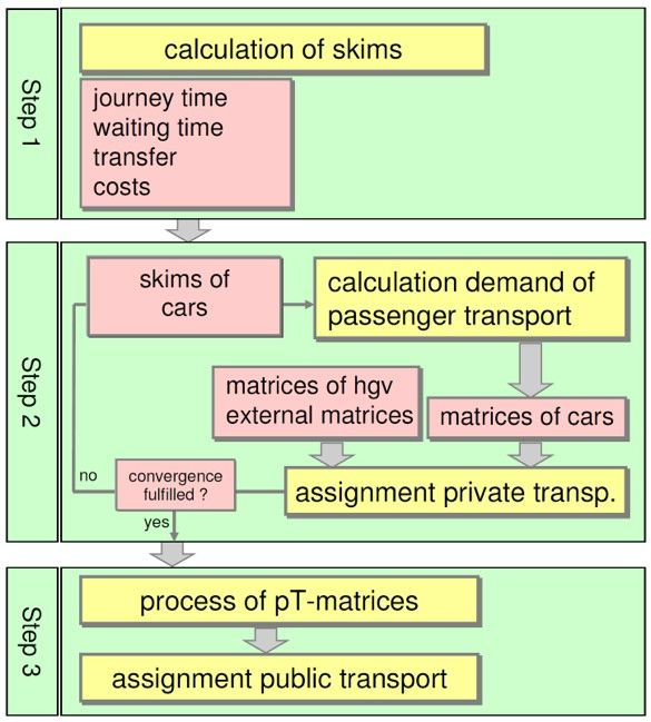
• 28,800 trips by 20,000 persons staying over night (private, with 3.6 trips/day, 40% pt
         share)

       • 6,400 trips by 20,000 one-day visitors (with 1.6 trips/day, 20% pt share)

For the above modeled groups of tourists, location choice is estimated by a gravitation model based
on 467 hotels, 277 places of interest, 1,957 restaurants, 311 museums and 41 shopping centers in
Berlin with the assumption over destination type shares of 40% places of interest, 25% restaurants,
15% museums and 20% shopping.

3.2    Modeling Process in VISUM

All the data sets mentioned above are assigned to the VISUM modeling process as shown in Fig-
ure 2(a). The generation of traffic demand matrices for individual transport is performed with EVA
(PTV Vision VISUM (PTV, 2012)). The demand is separated into 23 different groups defined
by their origin and destination activity types. For each of them, EVA splits the demand into the
four given transport modes (mit, pt, bike and walk) while using the resistance parameters: travel
time, distance costs, availability of the modes, parking costs, access/egress travel times and waiting
times as well as ride costs for public transport.

The static assignment process is split up into the VISUM iterative assignment process for mit
and the schedule based, none iterative assignment for pt. Therefore, the modeling process can be
described in three steps (see Figure 2(b)):

       1. Calculation of the necessary resistance parameters based on the street and public trans-
          port network

       2. Iterative calculation of demand and traffic assignment for mit

       3. pt assignment

The model is extensively validated and calibrated, based on data from the SrV travel survey (Ahrens
et al., 2009) as well as on the VBB 2007 public transport survey (VBB, 2008):

       • trip generation: Number of trips per demand group; validation of target activity distribu-
         tion for work and education

       • trip distribution: travel distances and travel times per demand group; traffic volumes
         per destination type and traffic zone as well as for selected screen lines; comparison of
         produced commuter trips with work statistics from the Bundesagentur für Arbeit (2008)

                                                  7
(a) VISUM process overview
(b) VISUM process steps
FIGURE 2 Macro-modeling process
8• mode choice: travel distances and travel times per mode-specific demand group; mode
share per demand group; overall mode share; comparison of the produced public trans-
port trips with the VBB survey data of 2007
• assignment (mit and pt): passenger volumes at train and bus stops; passenger volumes
per pt line (only subway, tram and bus); traffic volumes per line
4 Microscopic Modeling with MATSim
As shown in Figure 1 the outcome of the demand and static assignment model of VISUM is the
input for the modeling process in MATSim. In more detail, the micro-model has to respect
• the mit street network,
• the pt network, lines and their schedules,
• the zonal demographic population distribution,
• the zonal land use information,
• the zonal location choice distribution given by the 92 OD-matrices (4 transport modes
times 23 activity groups), and
• the additional demand from long distance, freight, airport and tourist traffic.
Since the zonal data for infrastructure, land use and population is too coarse for the microscopic
demand modeling process, additional land use information on block level is taken into account to
distribute potential activity locations inside zones. Finally, no activity-chain and timing informa-
tion is available from the trip based, static macro-model. Therefore, additional data sources have
to be added in the modeling process while respecting the distribution from the trip based demand.
All the above is part of the first step of MATSim’s scenario and initial individual demand modeling
process (MATSim-IIDM, Balmer (2007)) before the relaxation process (MATSim’s second step,
MATSim-EA, Balmer (2007)) can be performed.
4.1 Macro to Micro: Infrastructure data
The nodes of the VISUM network and their coordinates are directly converted into MATSim node
representations. For the street segments, the conversion process has to generate one or two directed
links (one-way / two-way street segments), and length, number of lanes, allowed transport modes,
9free speed, and link capacity are assigned to the generated links based on the attributes in the
VISUM data.
The public transport schedule, the lines, vehicles, and stops can be directly converted from the
VISUM model since its public transport assignment is schedule based. For some relations (e.g.
long distance trains) detailed vehicle information was incomplete. The conversion process then
used default values such that no artificial traffic bottleneck will occur during the simulation.
The static assignment in VISUM can be considered to be more robust against erroneous attributes,
especially considering links’ flow capacity. Due to the use of volume delay functions, links’ flow
capacities can be set too low (compared to reality) while only resulting in a slightly increased travel
time when running at full real capacity in the model. Especially on short links, this additional
travel time is often small enough to go undetected in macro models. In MATSim however, link
capacities are a hard constraint. Any capacity set too low will likely result in traffic jams during
the simulation.
Another common situation in network representations of macro models is that some street segment
attributes do not need to reflect reality if they are not used in the separate assignments for mit and pt.
Therefore, some post-processing has to be performed for the MATSim network: Some segments
define capacities and/or free speed equal to zero for mit mode (e.g. train tracks, closed streets or
oncoming traffic lanes in one-way streets). The mit mode type is removed in the MATSim network
representation for these links. In summary, 7,104 links with 0 values and 1,963 links with no
transport modes were removed from the mit network.
Other post-processing steps have to be performed for network links used by pt. Since MATSim
models and simulates the interaction of pt and mit traffic (Rieser, 2010), certain link attributes
have to be adapted to reflect the given pt schedules. Some link speeds define too low travel times
from one pt stop to another of a given pt line which would produce a service delay even on empty
streets. The free speed attributes of those links are increased to meet the schedules. Furthermore,
some link capacities used by pt are set too low such that pt vehicles would already produce spill
backs even without interaction with mit traffic. These links are typically located at entrance or exit
links of large bus stops like the bus stop at “Zoologischer Garten” in Berlin.
TABLE 1 Access and egress times and types per vehicle type
Vehicle type access time egress time access/egress type
[sec. per person and door] [sec. per person and door]
Ferry 2.00 2.00 serial
Bus 1.85 0.90 parallel
Tram 1.45 1.34 serial
Subway 1.31 1.12 serial
Suburban train 1.20 1.11 serial
Regional train 1.18 1.46 serial
Others/default 0.05 [per vehicle] 0.05 [per vehicle] serial
At last, MATSim also simulates access and egress delays at public transport stops, which are
dependent on the vehicle type, the number of doors and the door operation mode (Neumann and
10Nagel, 2010). These attributes are not available from the VISUM models. Based on passenger
surveys conducted by VSP in 2010 and 2011 (Neumann et al., 2011) the vehicle types are enriched
by this information as shown in Table 1.
4.2 Macro to Micro: Demand data
The target to produce the initial, individual demand for MATSim is to reflect the SrV survey
(Ahrens et al., 2009) while respecting the trip distribution of the macro model for each activity
group and for each mode of transport. The following paragraphs describe the process of the initial,
individual demand generation for the MATSim model.
4.2.1 SrV Survey to MATSim plans
In an initial step, the data from the SrV travel survey is converted into the MATSim plans format.
The conversion and filtering of the data is an important step since it (i) interprets the given raw
data and (ii) it makes it easier to work with it in later steps, where the travel demand has to be
distributed to the given population.
The household data set from the survey provides information about home location (on municipal-
ity and statistical zone level of detail), household size, number of cars, motorbikes and bicycles,
number of shared season tickets and income classes. The person data set contains the additional
information about age, gender, employment type, education type, driving license and public trans-
port user type (defines if a person uses public transport very often, seldom or never). This data
will later be used to define the demographic and socio-demographic description of each generated
agent and is also used to assign mit availability and season ticket ownership.
Finally, the trip table of the survey describes the activity chain of each person interviewed including
mode choice per trip, type of activity per destination, departure, travel and arrival time per trip, and,
therefore, also the activity duration per location and type. The geographic level of detail for each
destination is given by municipality and statistical zones.
4.2.2 VISUM to MATSim population
For each of the 1,537 traffic analysis zones of the VISUM model, the number of inhabitants of 30
socio-demographic homogenous groups (divided by age classes, employment or education type
and mit availability) is given. This information is converted into 4,436,363 synthetic persons
(MATSim agents) for the scenario with their home location distributed inside the zone accord-
ing to additional land use information on block level of detail.
114.2.3 Distribution of SrV plans to the MATSim population
A weighted draw of an SrV person is performed for each agent of the MATSim population. The
weighted draw is based on the geographic distribution as well as on the socio-demographic groups
defined by VISUM. For each agent, a choice set of potential SrV persons near to the agent’s home
location and of the same person group is created. Then, a random person is selected from that set
and his/her plan and demographic and socio-demographic attributes are assigned to the agent. This
procedure reflects the structural distribution of the activity-based demand of the survey in space
without being overly concerned about artifacts given by the zone borders.
4.2.4 Geocoding the Activity-Based Demand
This last step assigns a location for each activity of the activity-based demand (except for the
already assigned home location). In principle this can be called “location choice”. But since
the MATSim model has to reproduce the location choice already performed by the macro model
(stored in 92 OD-matrices), the process is therefore reduced to a weighted draw from the given
OD-matrices. For each trip of each MATSim plan, based on the given start and end activity, the
mode of transport and the traffic analysis zone of the start activity, the representing OD-matrix of
the VISUM model is selected and the destination zone is drawn by the distribution of the matrix.
For work and education activities, the procedure is done only once per plan and assigned to all
activities with the same type.
As a result, all activities are now assigned to a traffic analysis zone of the VISUM model. To assign
a coordinate inside the zones land use information on block level of detail is used in the same
manner as is done for the home locations. For the main activity types, i.e. work and education,
only a single coordinate is chosen per person and assigned to all main activities of the same type.
4.2.5 Comparison of the Initial, Individual Demand Modeling Process with the SrV
Survey Data
The quality of the produced initial demand can be compared directly with the travel survey data set.
Especially comparisons of distance distributions in total as well as for each mode of transport show
the quality of the activity chain distribution and also of the distribution of the chosen locations.
With that, this type of analysis also presents (in an indirect way) the quality of the location choice
of the macro model. Figure 3 shows that the differences are below 5% in total as well as for each
mode, which reflects the accuracy of the modeling process.
It is to mention that the figures shown here compare only the crow fly distances of the trips, since
reported travel distances are usually of low quality because of large errors in personal percep-
tions. To avoid this, the distances are calculated according to the post-processed geocoding of the
12mit pt bike walk mit pt bike walk
100% 100%
cumulative mode share
cumulative mode share
80% 80%
60% 60%
40% 40%
20% 20%
0% 0%
distance [m] distance [m]
(a) IIDM: cumulative distance distribution initial de- (b) SrV: cumulative distance distribution initial demand
mand
mit pt bike walk total
20%
15%
bias cumulative mode share
10%
5%
0%
0
100
200
500
1.000
2.000
5.000
10.000
20.000
50.000
100.000
-5%
-10%
-15%
-20%
distance [m]
(c) Bias cumulative distance distribution IIDM vs. SrV
FIGURE 3 Comparison of crow-fly distance distribution between IIDM and SrV survey
13reported trips. They are based on lower geographic resolution (municipality and statistical zone
level) but the error of perception can be eliminated.
4.3 Macro to Micro: Additional Traffic
Additional long distance, freight, airport and tourist traffic needs to be added to the MATSim
model. This is done by simply converting the given matrices from the VISUM model into addi-
tional “non-population representative” agents holding a single-trip plan with start and end activity
based on the given traffic analysis zones. Again, the coordinates inside the zones are chosen based
on building blocks.
4.4 MATSim Scenario Generation and Relaxation Process
At last, the demand has to be connected to the network. Since all activities contain a specific
coordinate and are not bounded to a zone anymore, the closest link to the coordinate is chosen as
entry and exit link of the mit mode while certain links are left out (e.g. motorways). For access to
the public transport infrastructure via pt stops, MATSim agents chose them automatically during
the relaxation process and therefore no assignment has to be done.
To take into account the various effects of the dynamic interaction in the traffic simulation, i.e.
traffic flow interaction and activity timing, the initial, individual demand generated above has to be
relaxed with MATSim’s co-evolutionary optimization process (Balmer et al., 2009). For the syn-
thetic population of the Berlin/Brandenburg Metropolitan Region the agents are able to optimize
in the dimensions route, time and mode choice. For the “non-population representative” agents
defining additional traffic only time and route choice is allowed to respect the predefined modes
from the macro model.
The utility function used to calculate the generalized utility of performed daily plans is based
on Charypar and Nagel (2005) but extended by additional terms for the different mode types.
Furthermore, monetary costs per transport mode are added to the function representing ticket and
acquisition costs for mit, bike, and pt. For public transport, agents determine the least cost path with
regards to walking time to and from pt stops, in-vehicle travel time, transfer time, waiting time, and
line switch costs. The model is calibrated and validated against the SrV travel survey with focus
on mode choice, travel time and travel distance distribution as well as on traffic volumes for pt
and mit by performing an experimental design method. The detailed description of the calibration
process is left out here since it would exceed the scope of this paper by far.
145 Comparison of Macro and Micro Model
This section focuses on the comparison between the macro and the micro model rather than the
validation to measured data, as an important goal of the project was to have two models similar
enough to exchange data between them.
TABLE 2 Public transport figures for macro and micro model - Subway, Tram, Bus and
Ferry values include BVG lines only
macro model micro model
total number of trips 3,230,792 3,577,075
total number of transfers 2,075,463 1,981,710
total number of passenger trips 5,306,255 5,558,785
total number of passenger trips - subway 1,710,603 1,414,513
total number of passenger trips - tram 490,176 524,081
total number of passenger trips - bus 1,211,724 1,600,294
total number of passenger trips - ferry 1,293 348
total number of passenger kilometer - subway 8,031,010 7,885,233
total number of passenger kilometer - tram 1,557,465 2,183,910
total number of passenger kilometer - bus 3,733,028 5,914,468
total number of passenger kilometer - ferry 1,274 1,038
average in-vehicle travel time per trip 17 min 45 s 20 min 07 s
average number of transfers per trip 0.642 0.554
total number of trips without transfers 1,548,525 1,950,921
total number of trips 1 transfer 1,316,325 1,306,173
total number of trips 2 transfers 339,799 284,648
total number of trips >2 transfers 26,143 35,333
share of trips without transfers 0.479 0.545
share of trips 1 transfer 0.407 0.365
share of trips 2 transfers 0.105 0.080
share of trips >2 transfers 0.008 0.010
Table 2 presents performance indicators used by BVG. First, the shares of different transport modes
operated by the BVG are compared. In general, the numbers match well. The macro model serves
slightly more trips with the subway lines, whereas the micro model serves more trips at the bus
network. Values for the tram network are nearly the same. Comparing the passenger-kilometers
and the passenger trips show shorter trips in the macro model for most transport systems. This is
underlined by the average in-vehicle travel time per trip, which differs by about three minutes. The
number of trips is slightly higher in the micro model, but the number of transfers is more or less the
same. This results in a higher number of transfers per trip in the macro model. In the micro model,
trips tend to be longer in travel time and distance. There are more trips served without transfers,
especially by the secondary network of bus and tram lines. This may be a direct consequence of
the models. Agents of the micro model can freely choose the stop to depart from based on their
activity location. Trips in the macro model start and end at connector links that are preset by the
network designer and limit the route choice, eventually eliminating connections without transfers.
As the pt values shown in Table 2 indicate, the traffic patterns of both models are comparable.
15(a) Macro model (b) Micro model
Berlin Metropolitan Area
Public Transport
Traffic volumes
macro model - micro model
(c) Difference of micro and macro model - A difference of less than 2000 trips per day is considered as
similar in both models.
FIGURE 4 Public transport traffic volumes in absolute values
16
% $# %
%
%
%
%
"
%%
%
%
!
%%
"%
!%
"
%%
%
%
%
% %
(a) Difference of micro and macro model in absolute values - A difference of less than 2000 trips
per day is considered as similar in both models.
( &
%"(
$'($
(
(
(
##((
(
(
# ((
$(
!(
( !
(
(
(
( (
(b) Difference of micro and macro model in relative values - A difference of less than 15 % is
considered as similar in both models.
FIGURE 5 Public transport traffic volumes - Detail of Alexanderplatz
17Figure 4(a) and 4(b) present the corresponding traffic volumes. As mentioned before, slight differ-
ences can be determined in the secondary network, especially in parts of the tram network in the
northeast. As the difference plot in Figure 4(c) illustrates, the micro model features more traffic at
the city train network, especially on its north-south and the west-east branches. The macro model
has more traffic at the southern part of the circle line and at parts of the subway network.
The more detailed view of the area of Alexanderplatz in Figure 5(a) shows the same amount of
traffic in both models for most lines. Only the part of the city train running from Jannowitzbrücke
to Hackescher Markt features more traffic in the micro model. The high absolute difference of the
city train in Figure 5(a) is not backed up by the complementing relative error shown in Figure 5(b).
The relative error for train, city train and subway lines are very small. Only the aforementioned
tram lines and some bus lines show a somewhat higher relative error, induced by low demand.
To conclude, both models show the same pt traffic pattern with the micro model featuring longer
trips, but with less transfers.
6 Behavioral Analyses
Given the high level of details in the micro-model, especially the availability of all the individuals’
attributes, a multitude of person group specific analyses can be performed. This section reports on
two of them to highlight the potential of microscopic models for public transport.
6.1 Demand analysis of a specific transit line
Consider a single bus line. The agents traveling with that line in the micro model can be easily
identified using MATSim’s output. Due to the nature of the model output, a number of interesting
questions can now be asked, especially such concerning the agents’ behavior over the simulated
day.
Figure 6 shows as an example the locations where agents that use the bus line 245 sometime
during their day are located at a specific time (see clock in figure), performing their activities. The
different colors represent different types of activities.
Similar pictures could be produced, showing other subsets of the population, e.g.:
• Show the current activity locations of persons using the bus line 245 during the morning
rush hour only.
• Show all work locations of persons using the bus line in the southbound direction.
18FIGURE 6 Current activity locations of agents traveling with bus line 245 sometime during
their day.
• Show all home locations of persons aged 25 to 65 using the bus line during 7 am and
7 pm.
Such analyses can help to better understand where passengers come from, where they are heading
to, and probably why they use a specific transit line and not another. It might also help to plan
optimal alternative lines if a line is regularly crowded.
6.2 Identifying potential transit demand
As mentioned earlier, all agents in the simulation have an attribute “public transport user type”.
This attribute reflects a person’s public transport usage pattern, differentiating persons that use
transit services often, seldom or never. For a transport company, the persons using the public
transport seldom are of high interest: Why are such persons not using the transit services more
often? How could those persons be influenced to use public transport more frequently?
Using the detailed output of the agent-based simulation MATSim, it is possible to extract the trips
of all agents having the public transport user type “seldom” and not using the public transport in
the simulation. For each trip, the route alternatives for using public transport or using a car or bike
can be calculated and compared to each other. Trips where the public transport route would take 2
or 3 times as long as the same trip performed with a car could be aggregated to some arbitrary zone
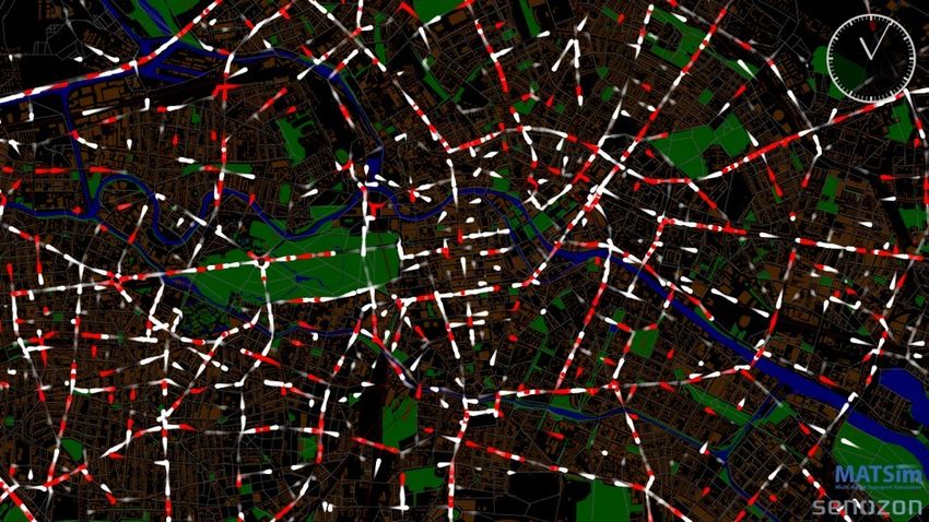
19FIGURE 7 Additional demand along line segments when occasional users are forced to use
public transport.
level of detail. The resulting OD matrix then depicts those OD relations where transit services are
not competitive, weighted by the actual demand. Thus, some slow but rarely used connections can
be easily identified in the matrix and ignored. Of higher interest are those OD connections with
a large entry in the matrix, as they represent slow or otherwise unattractive but often requested
connections.
Trying to get people use the public transport services could be done in different ways. If possible,
one could design new lines, increasing the connectivity of the public transport network. Typically,
this requires significant investments into the infrastructure and/or vehicle fleet and an increase
in operational cost. Such a change is thus not always possible or only in the long term. On
the other hand, one could try to extract those OD relations where public transport is slower by
a small fraction only and try to convince people to use the transit offerings e.g. by means of
advertisement. This might be feasible on a much shorter time scale and with a smaller budget.
To prevent overcrowding of existing transit lines, the simulation can calculate which lines these
occasional users would travel with, and also check which lines have most unused capacity, to make
potential measures even more specific to a certain person group. Figure 7 shows the additional
demand along line segments when all occasional users are forced to use public transport, thus
highlighting possible future bottlenecks.
207 Conclusion and Outlook
This paper presented the successful transformation of a static macroscopic model into an inte-
grated activity based demand and dynamic assignment model performed for a real application on
the Berlin/Brandenburg Metropolitan Region. While the two models clearly differ in their method-
ology overall key values can be reproduced showing similar results. Furthermore, it is shown that
by the use of the activity chain distributions and their timing activity based demand can be repro-
duced with respect to the trip distribution of the origin-destination matrices from VISUM. From
the view of the “Berliner Verkehrsbetriebe” BVG the process flow defined for this project allows
them to use both models for planning purpose, case studies and effect analysis while modeling
their needs in the VISUM editor environment and performing the model calculation in VISUM as
well as in MATSim. As a result they are able to analyze effects on the macroscopic level of detail
as well as on agent-based level to capture specific customer groups and/or time ranges during the
day. Since the traffic flow simulation also takes into account the interactions between mit and pt
the BVG is also able to analyze disturbances of the public transport schedules on an operative level
(e.g. due to congestions of car traffic, delays of access and egress times of passengers, and so on).
Nevertheless, some issues occurred in this project have to be addressed:
Network representation: The models interpret transportation networks differently which pro-
duces a certain lack of consistency. While the MATSim model is very restrictive about its link
attribute values, which have direct influence in the traffic flow simulation, some attributes in the
macro model do not affect the assignment process. This clearly recalls the fact that the assignment
process of the macro model is separated for the different transportation modes but treated in a
multi-modal way in the simulation. As an example, there is not always a clear distinction between
buses or trams using same or different lanes than cars on a street segment. But for the MAT-
Sim network representation, this would be of importance since the street segment would either be
combined into one link with both modes or separated into two links with one mode per link. To
overcome this problem, the macroscopic network has to be extended by this kind of information.
Reconstruction of the activity based demand on the base of origin-destination matrices: The
join of the two data sources presented in this paper works very well. But it has to be stated that
the used data sets—especially the travel survey data set—are the base for both demand modeling
processes and therefore, fit very well together. It is unclear to this point if the proposed process
step will work in every case, i.e. when the data sources are not of that high level of quality and
quantity.
Process flow: The process flow presented in this paper suits very well for real world applications
and effect analysis for the BVG and is consistent within the generation processes of both models.
From a conceptual point of view, the process steps should be reorganized since the reconstruction
of activity-based demand with the basis of the trip based demand by VISUM is actually a detour.
To gain the advantages of both models without this detour, we would suggest the following:
1. Modeling of population, land use, transportation networks and schedules with VISUM
21using the advantages of various modeling and editor features provided by the software.
2. Modeling the initial, individual, activity-based demand using MATSim (or with other
activity-based models, i.e. Bhat et al. (2004); Roorda et al. (2008); Arentze and Tim-
mermans (2004), etc.).
3. Compute, calibrate and validate the demand with the co-evolutionary relaxation pro-
cess of MATSim using at least all four choice dimensions (routes, times, modes, and
locations).
4. Convert the relaxed demand into zone based origin-destination matrices (similar to the
work presented in (Gao et al., 2010).
5. Run the traffic assignment for the different modes with VISUM.
6. Analyze the outcome again on both tracks; for the macro and micro model.
With this suggestion, no reconstruction of the activity-based demand has to be done and both
models deliver full functionality for the user. The main reason for the process steps presented here
is that the BVG already receives a complete VISUM model without dependencies to the fairly
new approach with MATSim. Nevertheless, the proposed “get-together” of a macroscopic and an
activity-based, microscopic transport model delivers valuable findings for various questions and
applications for the BVG.
Acknowledgments
We would like to thank BVG and in particular Heinz Krafft-Neuhäuser for providing the data, and
the group of Prof. H. Schwandt, in particular Norbert Paschedag, at the Department of Mathe-
matics at TU Berlin for maintaining our computing clusters. Furthermore, we would like to thank
PTV Berlin, namely Siegurd Müller and Hartmut Kästner, who modeled the macroscopic part of
the project. The travel survey data was provided with the help of Imke Steinmeyer from Senatsver-
waltung für Stadtentwicklung Berlin and was further enriched by the group of Frank Ließke at VIP
TU Dresden. Finally, we would like to thank Prof. Kai Nagel for the support in this project on the
part of TU Berlin.
22References
Ahrens, G.-A., F. Liesske, R. Wittwer, and S. Hubrich (2009). Endbericht zur verkehrserhebung
“mobilität in städten – srv 2008” und auswertungen zum srv-städtepegel. final report, Techni-
cal University Dresden, Dresden. URL http://tu-dresden.de/die_tu_dresden/
fakultaeten/vkw/ivs/srv/dateien/staedtepegel08_akt.
Arentze, T. and H. Timmermans (2004). A learning-based transportation oriented simulation sys-
tem. Transportation Research Part B, 38:613–633.
Axhausen, K. and T. Gärling (1992). Activity-based approaches to travel analysis: conceptual
frameworks, models, and research problems. Transport Reviews, 12(4):323–341.
Axhausen, K. and R. Herz (1989). Simulating activity chains: German approach. Journal of
Transportation Engineering, 115(3):316–325.
Balmer, M. (2007). Travel Demand Modeling for Multi-Agent Traffic Simulations: Algorithms and
Systems. PhD thesis, ETH Zurich, Zurich.
Balmer, M., M. Rieser, K. Meister, D. Charypar, N. Lefebvre, and K. Nagel (2009). MATSim-T:
Architecture and simulation times. In Bazzan, A. L. C. and F. Kluegl, editors, Multi-Agent Sys-
tems for Traffic and Transportation Engineering, pages 57–78. Information Science Reference,
Hershey.
Beckx, C., T. Arentze, L. Int Panis, D. Janssens, J. Vankerkom, and G. Wets (2009). An in-
tegrated activity-based modelling framework to assess vehicle emissions: approach and ap-
plication. Environment and Planning B: Planning and Design, 36(6):1086–1102. URL
http://www.envplan.com/abstract.cgi?id=b35044.
Ben-Akiva, M., M. Bierlaire, H. Koutsopoulos, and R. Mishalani (2002). Real time simulation of
traffic demand-supply interactions within DynaMIT. In Gendreau, M. and P. Marcotte, editors,
Transportation and network analysis: current trends: miscellanea in honor of Michael Florian,
pages 19–36. Kluwer Academic Publishers.
Bhat, C., J. Guo, S. Srinivasan, and A. Sivakumar (2004). A comprehensive econometric mi-
crosimulator for daily activity-travel patterns. Transportation Research Record, 1894:57–66.
Bradley, M., J. Bowman, and B. Griesenbeck (2010). SACSIM: An applied activity-based model
system with fine-level spatial and temporal resolution. Journal of Choice Modeling, 3(1):5–31.
Bundesagentur für Arbeit (2008). Sozialversicherungspflichtig Beschäftigte - Pendlerdaten,
Berichtsmonat Juni 2008. Technical report, Bundesagentur für Arbeit.
BVG (2012). Berliner Verkehrsbetriebe – Anstalt des öffentlichen Rechts. http://www.bvg.de.
URL http://www.bvg.de.
Charypar, D. and K. Nagel (2005). Generating complete all-day activity plans with genetic algo-
rithms. Transportation, 32(4):369–397.
23Ettema, D., G. Tamminga, H. Timmermans, and T. Arentze (2005). A micro-simulation model
system of departure time using a perception updating model under travel time uncertainty.
Transportation Research Part A: Policy and Practice, 39(4):325–344. ISSN 0965-8564. doi:
DOI:10.1016/j.tra.2004.12.002. URL http://www.sciencedirect.com/science/
article/pii/S0965856404001144. Connection Choice: Papers from the 10th IATBR
Conference.
Fellendorf, M., T. Haupt, U. Heidl, and W. Scherr (1997). Ptv vision: Activity-based micro-
simulation model for travel demand forecasting. In Ettema, D. F. and H. J. P. Timmermans,
editors, Activity-Based Approaches to Travel Analysis, pages 55–72. Pergamon, Oxford.
Gao, W., M. Balmer, and E. Miller (2010), Comparisons between MATSim and EMME/2 on
the Greater Toronto and Hamilton Area network. In TRB, editor, 89th Annual Meeting of the
Transportation Research Board, Washington, D.C. (2010). Transportation Research Board.
Horni, A., D. Scott, M. Balmer, and K. Axhausen (2009). Location choice modeling for shop-
ping and leisure activities with MATSim: Combining micro-simulation and time geography.
Transportation Research Record, 2135:87–95.
Lin, D.-Y., N. Eluru, S. Waller, and C. Bhat (2008). Integration of activity-based modeling and
dynamic traffic assignment. Transportation Research Record, 2076:52–61.
MATSim (2012). Multi-Agent Transportation Simulation Toolkit. http://www.matsim.org. URL
http://www.matsim.org.
Meister, K. (2011). Contribution to agent-based demand optimization in a multi-agent transport
simulation. PhD thesis, ETH Zurich, Zurich.
Neumann, A. and K. Nagel (2010). Avoiding bus bunching phenomena from spreading: A dynamic
approach using a multi-agent simulation framework. VSP Working Paper 10-08, Berlin Insti-
tute of Technology. URL https://svn.vsp.tu-berlin.de/repos/public-svn/
publications/vspwp/2010/10-08. see www.vsp.tu-berlin.de/publications.
Neumann, A., S. Kern, and K. Nagel (2011). Boarding and alighting time of passengers of the
berlin public transport system. Technical report, Berlin Institute of Technology, Transport Sys-
tems Planning and Transport Telematics. forthcoming.
Ortúzar, J. d. D. and L. Willumsen (2001). Modelling transport. John Wiley Sons Ltd, Chichester,
3rd edition.
Peeta, S. and A. Ziliaskopoulos (2001). Foundations of Dynamic Traffic Assignment: The Past,
the Present and the Future. Networks and Spatial Economics, 1(3):233–265. doi: 10.1023/A:
1012827724856.
PTV (2003). Integriertes Verkehrsentwicklungsprojekt fuer die Region Usedom - Wollin: FoPS
Projekt.Nr. 70.0718/2003. short report, Bundesministerium für Verkehr, Bau und Stadten-
twicklung, Bonn. URL http://www.mobilitaet21.de/uploads/tx_userumm21/
Kurzfassung_Usedom_Wollin_180106.pdf.
24PTV (2012). PTV AG: traffic, mobility, logistics. http://www.ptv.de. URL http://www.ptv.
de.
Rieser, M. (2010). Adding Transit to an Agent-Based Transportation Simulation. PhD thesis,
Berlin Institute of Technology, Berlin.
Rieser, M., K. Nagel, U. Beuck, M. Balmer, and J. Rümenapp (2007). Truly agent-oriented cou-
pling of an activity-based demand generation with a multi-agent traffic simulation. Transporta-
tion Research Record, 2021:10–17. doi: 10.3141/2021-02.
Roorda, M. J., E. J. Miller, and K. Habib (2008). Validation of TASHA: A 24-h activity
scheduling microsimulation model. Transportation Research Part A: Policy and Practice,
42(2):360 – 375. ISSN 0965-8564. doi: DOI:10.1016/j.tra.2007.10.004. URL http:
//www.sciencedirect.com/science/article/pii/S0965856407000924.
Senatsverwaltung für Stadtentwicklung Berlin (2009). Gesamtverkehrsprognose 2025 für die Län-
der Berlin und Brandenburg. Technical report, Ministerium für Infrastruktur und Raumordnung
Brandenburg, Berlin.
Senozon (2012). Senozon AG: understanding mobility. http://www.senozon.com. URL http:
//www.senozon.com.
Sheffi, Y. (1985). Urban Transportation Networks: Equilibrium Analysis with Mathematical Pro-
gramming Methods. Prentice-Hall, Englewood Cliffs, NJ, USA.
VBB (2008). Verkehrserhebung 2005, Berlin. Technical report, Verkehrsverbund Berlin Branden-
burg.
Vrtic, M. and K. Axhausen (2003). Experiment mit einem dynamischen Umlegungsverfahren.
Strassenverkehrstechnik, 47(3):121–126. Also Arbeitsberichte Verkehrs- und Raumplanung
No. 138, see www.ivt.baug.ethz.ch.
VSP (2012). Transport Systems Planning and Transport Telematics, Berlin Institute of Technology.
http://www.vsp.tu-berlin.de. URL http://www.vsp.tu-berlin.de.
Watling, D. (1996). Asymmetric problems and stochastic process models of traffic assignment.
Transportation Research B, 30(5):339–357.
Ziliaskopoulos, A. K. and S. T. Waller (2000). An internet-based geographic information sys-
tem that integrates data, models and users for transportation applications. Transportation Re-
search Part C: Emerging Technologies, 8(1-6):427–444. ISSN 0968-090X. doi: DOI:10.
1016/S0968-090X(00)00027-9. URL http://www.sciencedirect.com/science/
article/pii/S0968090X00000279.
25You can also read