Design Method of Differential Cascading for Dual-Stator Brushless Doubly-Fed Induction Wind Generator With Staggered Dual Cage Rotor
←
→
Page content transcription
If your browser does not render page correctly, please read the page content below

ORIGINAL RESEARCH
                                                                                                                                published: 15 September 2021
                                                                                                                               doi: 10.3389/fenrg.2021.749424

                                           Design Method of Differential
                                           Cascading for Dual-Stator Brushless
                                           Doubly-Fed Induction Wind Generator
                                           With Staggered Dual Cage Rotor
                                           Yu Zeng, Ming Cheng *, Xiaoming Yan and Changguo Zhang
                                           School of Electrical Engineering, Southeast University, Nanjing, China

                                           This article proposes a new differential-cascading-based dual-stator brushless doubly-fed
                                           induction machine with a staggered dual cage rotor. Conventional differential mode of the
                                           brushless doubly-fed machine with cage rotor suffers from the low number of rotor bars
                                           because of the low equivalent synchronous pole pairs of |p1-p2|, and thus, severe rotor flux
                                           leakage, low capacity of magnetic field conversion of the rotor and low efficiency. To
                                           overcome the obstacle of the excessive harmonics of the rotor, a design method based on
                                           the differential cascading is proposed which enables the cage rotor with a high number of
                            Edited by:
                       Liansong Xiong,     conductor bars even in the case of low pole pairs of |p1-p2|, hence the greatly reduced
Nanjing Institute of Technology (NJIT),    rotor leakage inductance and enhanced performance of the machine. The rotating
                                 China
                                           magneto-motive force theory is applied to derive the interconnection rule of the
                       Reviewed by:
                     Qingsong Wang,
                                           staggered dual cage rotor, and meanwhile, the corresponding examples are illustrated.
          Southeast University, China      The performance comparisons between the differential cascading and the sum cascading
                     Ramtin Sadeghi,       based on the proposed machine are carried out. The results show that the proposed
                             IAU, Iran
                               Lei Liu,    machine based on the differential cascading obtains higher power densities comparing to
      Xi’an Jiaotong University, China     the sum cascading at the region of sub-natural synchronous speed, while its drawback is
                  *Correspondence:         the increment of the loss due to the high rotor frequency, gaining lower efficiencies at the
                        Ming Cheng         region of super-natural synchronous speed.
                 mcheng@seu.edu.cn
                                           Keywords: brushless doubly-fed generator, wind turbine, generators, conductors, cage rotors
                   Specialty section:
        This article was submitted to
        Process and Energy Systems         INTRODUCTION
                          Engineering,
               a section of the journal    Brushless doubly-fed machines (BDFMs), as the alternative to the conventional doubly-fed induction
         Frontiers in Energy Research      machine (DFIM) (Yin, 2021; Zhang et al., 2021), offer increased reliability and low maintenance due
            Received: 29 July 2021         to the elimination of the brushes and slip-rings (Okedu et al., 2021), showing the promising prospects
        Accepted: 31 August 2021           in the fields of variable speed constant frequency system (VSCF) such as the on-shore and off-shore
     Published: 15 September 2021
                                           wind power generation system (Cheng and Zhu, 2014; Han et al., 2018; Xiong et al., 2020). The
                            Citation:      critical technology of the BDFM is the structure design of the rotor which determines the capacity of
Zeng Y, Cheng M, Yan X and Zhang C         the magnetic field conversion between the power subsystem and the control subsystem. Therefore,
 (2021) Design Method of Differential
                                           lots of feasible rotor topologies have been investigated by researchers from academia and industry
 Cascading for Dual-Stator Brushless
Doubly-Fed Induction Wind Generator
                                           like the nested-loop rotor (Shao et al., 2012), the wound rotor (Ruviaro et al., 2011), and the
   With Staggered Dual Cage Rotor.         reluctance rotor (Zhang et al., 2019). A relatively new machine with dual-stators and dual-rotors
        Front. Energy Res. 9:749424.       called the dual-stator brushless doubly-fed induction machine (DS-BDFIM) has been developed in
    doi: 10.3389/fenrg.2021.749424         recent years which offers the merits of low harmful harmonics and good winding insulation.

Frontiers in Energy Research | www.frontiersin.org                                 1                                September 2021 | Volume 9 | Article 749424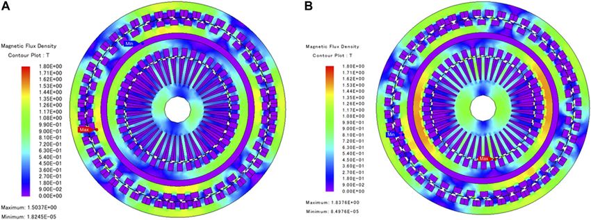
Zeng et al.                                                                                                       Differential Cascading for DS-BDFIG

However, the capacity of the magnetic field conversion for the               pairs. The problem that should be addressed now is the
cascaded wound rotor seems to be low due to the relatively high             interconnection of the rotor conductor bars to produce the
rotor resistance (Zeng et al., 2021). To reduce the copper loss of          same direction of rotation for two main magnetic fields and
the rotor and improve the efficiency of the DS-BDFIM, back to                build so-called differential cascading (DC).
the structure of the cage rotor is a potential solution.                        In this article, the design method of DC for the DS-BDFIM with a
Consequently, in this article, the DS-BDFIM with cage rotor is              staggered dual cage rotor (DS-BDFIM-SDCR) is proposed. The
studied.                                                                    number of conductor bars of DS-BDFIM-SDCR based on the DC
    No matter what kinds of rotor structures used in previous               is in accordance with the sum cascading (SC) one which means the
literature, two main magnetic fields produced by the rotor are               number of conductor bars large even with the pole pairs of |p1-p2|,
generally opposite, constructing the synchronous machine with               hence the greatly reduced rotor leakage inductance and improved
equivalently (p1+p2) pole pairs and the natural synchronous                 performance of the machine. The theoretical derivation of the
speed of the BDFM is 60f1/(p1 + p2). The operation principle                interconnection rule of the DS-BDFIM-SDCR based on the DC is
is the so-called sum mode. By that analogy, if a magnetic field of           developed in Design Method of DC. The specific pole/slot
the rotor rotates in the same direction with respect to the other           combinations are introduced in Slot/Pole Combinations of DS-
one, the natural synchronous speed of the BDFM is determined                BDFIM-SDCR in detail. The advantage of the wide speed range
by 60f1/|p1-p2| and the pole pairs are equivalent to be |p1-p2|             and the disadvantage of the increased loss are discussed in
which has been pointed out in (Williamson et al., 1997), namely,            Comparison of DS-BDFIM-SDCR with DC and SC, and
the differential mode of the BDFM. Since n ∝ 1/p (where p                   meanwhile, the finite element (FE) models of the DC and SC
indicates the (p1 + p2) in the sum mode of the BDFM and the |p1-            modes of the DS-BDFIM-SDCR are established to compare their
p2| in the differential mode of the BDFM, while n is the                    performances. Finally, the vital conclusion is drawn in Conclusion.
synchronous speed of the machine), the synchronous speed of
the differential mode of the BDFM is higher than the sum mode
one. The higher synchronous speed owns the increased power                  DESIGN METHOD OF DC
density of the machine. It means that the differential mode of the
BDFM has the potential ability of higher power density                      Structure of DS-BDFIM-SDCR
comparing to the sum mode of the BDFM. Moreover, a wider                    The DS-BDFIM-SDCR consists of the outer stator, the inner
range of speed for the differential-mode-based BDFM is                      stator and the cup-shaped rotor as shown in Figures 1A,B. The
significantly beneficial for the wind power generation in a                   power winding (PW) is placed in the slotted outer stator to output
complex environment.                                                        power, while the control winding (CW) is wrapped around the
    The key to restricting the development of the differential mode         inner stator to account for the slip power. The cup-shaped rotor is
of the BDFM is the severe rotor flux leakage. In the early study             made of the inner cage rotor, the outer cage rotor and the non-
(Williamson et al., 1997), the cage rotor is utilized for the               magnetic support in between, termed as the SDCR. The non-
differential-mode-based BDFM, but the number of rotor bars                  magnetic support enables the electric coupling instead of the
is too low owing to the low pole pairs of |p1-p2|, resulting in             magnetic coupling between the inner and outer cage rotors,
excessive harmonics and the large rotor leakage inductance.                 achieving the cascaded principle rather than the modulation
Although Robert P. C. reported in (Roberts, 2004) that the                  one. More details about the SDCR is presented in Figure 1C,
rotor leakage inductance can be declined when the appropriate               showing that on the one end the conductor bars of the inner and
design method is adopted, there is little hope of success for the           outer cages are shorted-circuited by two end rings, whereas on the
nested-loop and the reluctance rotors (Li et al., 2019). To solve the       other end they are interconnected in a staggered way to form the
problem of the excessive harmonics of the rotor, Cheng Y. utilized          same rotating magnetic fields, namely, the DC. It is worth
the special design method for the wound rotor to reduce the                 mentioning that the real 3-dimension topology of 40 staggered
harmonic content (Cheng et al., 2020). The reasonable wound                 conductor bars (40 slots of the rotor for the proposed machine) is
winding design indeed can reduce the rotor harmonics, however,              a little bit complex, and hence, the simplified view (only for
the high rotor resistance is a prevalent obstacle that the wound            reference) is provided for a clear illustration. The design
rotor usually experiences, leading to high copper loss. Further, the        parameters of the proposed DS-BDFIG-SDCR are tabulated in
rotor current frequency of the differential-mode-based BDFM is              Table 1. Obviously, the equivalent synchronous 1 pole pair and
much higher than the sum mode one, leading to the increased                 the 40 slots of the rotor (namely, the number of the conductor
rotor copper loss and iron loss (Pan et al., 2020). To overcome the         bars) heavily reduce the rotor flux leakage and harmonics.
drawbacks of the wound rotor, the cage rotor structure with low             Therefore, the obstacle of the differential mode for the
resistance should be reconsidered. BDFMs can be divided into                conventional BDFIM with the cage rotor is removed in a sense.
two categories in terms of the operating principle, namely, the
class of modulation and the class of cascaded (Zeng et al., 2020).
Williamson S. verified that the differential mode is not                     Derivation of Interconnection Rule for
appropriate to the nested-loop rotor with the modulation                    SDCR
principle (Williamson et al., 1997). Therefore, the cascaded                The cage winding can be treated as a balanced multi-phase
cage rotor is supposed to be investigated to realize the purpose            winding whose phase and slot numbers are the same. The
of the rotor with a large number of conductor bars under low pole           number of conductors for each phase is 1. Since the

Frontiers in Energy Research | www.frontiersin.org                      2                                 September 2021 | Volume 9 | Article 749424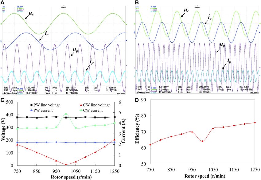
Zeng et al.                                                                                                                        Differential Cascading for DS-BDFIG

  FIGURE 1 | Structure of DS-BDFIM-SDCR (A) Three-dimensional view (B) Cross-sectional view (C) Simplified view of staggered dual squirrel cages (for reference
  only).

TABLE 1 | Specification of proposed DS-BDFIM-SDCR

Design parameters                                                       Values

PW and CW pole pairs                                                      2, 1
Slot number of outer stator and outer rotor                              48, 40
Slot number of inner rotor and inner stator                              40, 36
Rated PW voltage (V)                                                      220
Rated frequencies of PW and CW (Hz)                                    50, 12.5
Rated speed (r/min)                                                      3,750
Outer and inner diameters of outer stator (mm)                         325, 277
Outer and inner diameters of outer rotor (mm)                          276, 231
Thickness of non-magnetic support (mm)                                     9
Outer and inner diameters of inner rotor (mm)                          213, 159
Outer and inner diameters of inner stator (mm)                          158, 40
Axial length of stator core (mm)                                          246

conductors are symmetrically distributed, the current amplitudes
and the current frequencies of the conductor bars are the same.
However, their phase angles are different. The electric phase angle
of the current for the adjacent conductor bars is defined as
                                        2πpc
                                  α                                         (1)
                                         Zc
And because of the conductor bars arranged symmetrically along                          FIGURE 2 | Equivalent topology of SDCR.
the circumference of the rotor in space, the adjacent conductor
bars differ a phase angle β in space
                                       2πpp
                                  β                                         (2)
                                        Zp
                                                                                       of the outer and inner rotors. The equivalent topology of the
where p p and pc are respectively given as the pole pairs of the                       SDCR is given in Figure 2, explaining the relation of inner and
PW and the CW, while Zp and Zc represent the number of slots                           outer cages.

Frontiers in Energy Research | www.frontiersin.org                                 3                                      September 2021 | Volume 9 | Article 749424
Zeng et al. Differential Cascading for DS-BDFIG
If the balanced m phases currents are injected into the Substituting Eq. 9 into Eq. 8, the synthetic MMF is finally
balanced m phases cage winding, the fundamental magneto- given by
motive forces (MMFs) are given by ⎪
⎧ m m ⎪
⎫
⎪
⎪ ⎪
⎪
⎪
⎪ ⎜
⎛
⎜ 1 + 1 + /1 1 + 1 + /1⎞ ⎟
⎟ ⎪
⎪
⎪
⎧ f1 Fm sin(ωt)sin(x) ⎪
⎪ ⎜
cos(ωt − x)⎜
⎝ + ⎟
⎟
⎠ ⎪
⎪
⎪ ⎪
⎪ ⎪
⎪
⎪
⎪ f2 Fm sin(ωt − α)sinx − β ⎪
⎪ 2 2 ⎪
⎪
⎪
⎨ ⎪
⎪ ⎪
⎪
⎪
⎪ ⎪
⎪
⎪ f3 Fm sin(ωt − 2α)sinx − 2β (3) ⎪
⎪ ⎪
⎪
⎪
⎪ ⎪
⎪ ⎪
⎪
⎪
⎪ « ⎪
⎪ m−1
m−1
⎪
⎪
⎩ ⎪
⎪ + + /1 + + /1 ⎪
⎪
fm Fm sin[ωt − (m − 1)α]sinx − (m − 1)β ⎪
⎪ ⎝
⎛ 1 1 1 1 ⎠
⎞ ⎪
⎪
1 ⎨ +sin(ωt − x) − ⎬
f Fm ⎪ 2i 2i
⎪ (10)
2 ⎪ ⎪ ⎪
⎪
where Fm is the amplitude of the fundamental MMF. ⎪
⎪ ⎪
⎪
⎪
⎪ ⎪
⎪
Making a summation of all MMFs from Eq. 3 and using the ⎪
⎪ 1 1−1 1 1−1 ⎪
⎪
⎪
⎪ −cos(ωt + x)
+ ⎪
⎪
product-to-sum formulas of the trigonometric function, the ⎪
⎪ i(α+β) −i(α+β) ⎪
⎪
⎪
⎪
2 1 − e 2 1 − e ⎪
⎪
synthetic MMF can be derived as ⎪
⎪ ⎪
⎪
⎪
⎪ ⎪
⎪
⎪
⎪ i ( )−1 1 e ( )−1 ⎪
α+β −i α+β ⎪
⎪
⎧ cos(ωt − x)1 + cosα − β + cos2α − β + / + cos(m − 1)α − β ⎪
⎫ ⎪
⎪ 1 e ⎪
⎪
⎪ ⎪
⎩ −sin(ωt + x)
2i 1 − ei(α+β) − 2i 1 − e−i(α+β) ⎪
⎪
⎪ ⎪
⎪ ⎪
⎪
⎪ ⎪
⎪ ⎭
1 ⎪ ⎨ +sin(ωt − x)sinα − β + sin2α − β + / + sin(m − 1)α − β ⎪
⎬
f Fm ⎪ ⎪
2 ⎪ ⎪ −cos(ωt + x)1 + cosα + β + cos2α + β + / + cos(m − 1)α + β ⎪
⎪
⎪
⎪ ⎪
⎪
⎪
⎩ ⎪
⎭ Eq. 10 can be simplified further
−sin(ωt + x)sinα + β + sin2α + β + / + sin(m − 1)α + β
⎪
⎧ m m m−1 m−1 ⎫ ⎪
(4) ⎪ cos(ωt − x) 2 + 2 ! + sin(ωt − x) 2i − 2i ! ⎪
⎪ ⎪
1 ⎪ ⎨ ⎪
⎬ m
On the basis of Euler’s formula f Fm ⎪ ⎪ Fm cos(ωt − x)
2 ⎪ ⎪ ⎪
⎪ 2
⎪ 1 1
⎩ −cos(ωt + x)(0 + 0) − sin(ωt + x) − + ! ⎪
⎭
eiθ cos(θ) + isin(θ) (5) 2i 2i
(11)
Eqs. 6, 7 are easily derived where ωt-x is defined as the positive rotation of the magnetic field,
iθ −iθ while ωt + x represents the negative rotation. The physical
e +e meaning of Eq. 11 is that the inner and outer conductor bars
cos(θ) (6)
2 are interconnected in a positive-phase sequence to produce the
e − e−iθ
iθ
same rotation direction of the magnetic fields of the rotor
sin(θ) (7)
2i currents, namely, the so-called DC.
According to Eqs. 4, 6, 7, the synthetic MMF is rewritten as
⎪
⎧ 1 + ei(α−β) + ei2(α−β) + / + ei(m−1)(α−β) ⎪
SLOT/POLE COMBINATIONS OF
⎪
⎪ ⎢
⎡
⎢ ⎤⎥⎥⎥ ⎫ ⎪
⎪
⎪ ⎢
⎢
⎢
⎢ 2 ⎥⎥⎥ ⎪ ⎪
⎪ DS-BDFIM-SDCR
⎪
⎪ ⎢
⎢ ⎥⎥⎥ ⎪
⎥ ⎪
⎪
⎪ cos(ωt − x) ⎢
⎢
⎢ ⎥ ⎪
⎪
⎪
⎪ ⎢
⎢
⎢ −i(α−β) −i2(α−β) −i(m−1)(α−β) ⎥
⎥
⎥ ⎪
⎪
⎪
⎪ ⎣ 1+e +e +/+e ⎦ ⎪
⎪ α and β represent the electric phase angles of the slots in the CW
⎪
⎪ + ⎪
⎪
⎪
⎪ ⎪
⎪
⎪
⎪ 2 ⎪
⎪ and the PW sides and they are should be the same under the DC
⎪
⎪ ⎪
⎪
⎪
⎪ ei( α−β ) + e i2 ( α−β ) + / + ei(m−1) (α−β) ⎪
⎪
⎪
⎪ ⎢
⎡ ⎥⎥⎥
⎤ ⎪
⎪ 2πpp 2πpc
⎪
⎪ ⎢
⎢⎢
⎢ ⎥ ⎪
⎪ βα
⎪
⎪ ⎢⎢⎢ 2i ⎥
⎥⎥⎥ ⎪
⎪ (12)
⎪
⎪
⎪ +sin(ωt − x) ⎢
⎢ ⎥
⎥ ⎪
⎪
⎪ Zp Zc
⎪
⎪ ⎢
⎢
⎢⎢⎣ −i(α−β) ⎥
⎥ ⎪
⎪
⎪ −i2(α−β) −i(m−1)(α−β) ⎥ ⎥
⎦ ⎪
⎪
⎪ e +e +/+e ⎪
⎪ Then, the requirement of the slot/pole combination of the PW
⎪ − ⎪
1 ⎪ ⎨ 2i
⎪
⎬ and CW is gained
f Fm ⎪ ⎪
2 ⎪ ⎪ 1+e i( α+β ) +e i2 ( α+β ) +/+e i(m−1) ( α+β ) ⎪
⎪ pp Zc pc Zp
⎪
⎪ ⎢
⎡ ⎥
⎤ ⎪
⎪ (13)
⎪
⎪ ⎢
⎢ ⎥
⎥
⎥ ⎪
⎪
⎪
⎪ ⎢
⎢ ⎥ ⎪
⎥⎥⎥ ⎪
⎪ ⎢ 2 ⎥ ⎪ The steady-state speed of the DS-BDFIM-SDCR based on the DC
⎪ −cos(ωt + x) ⎢⎢⎢ ⎪
⎪
⎪ ⎢ ⎥ ⎪
⎪ ⎢
⎢⎢⎢ ⎥⎪
⎥
⎪
⎪
⎪ ⎣ 1 + e−i(α+β) + e−i2(α+β) + / + e−i(m−1)(α+β) ⎥⎥⎦ ⎪ ⎪
⎪
⎪
is given by
⎪
⎪ + ⎪
⎪
⎪
⎪
⎪ 2 ⎪
⎪
⎪
60"fp ± fc #
⎪
⎪
⎪
⎪
⎪
⎪ nr $$$ $$ (14)
⎪
⎪
⎪
⎪ ⎡
⎢
ei( α+β ) + e i2 ( α+β ) + / + ei(m−1) (α+β)
⎤
⎥
⎪
⎪
⎪
⎪
$$pp − pc $$$
⎪
⎪ ⎢⎢⎢ ⎥⎥⎥ ⎪
⎪
⎪
⎪ −sin(ωt + x)⎢⎢ ⎢
⎢ 2i ⎥
⎥ ⎪
⎪
⎪
⎪ ⎢ ⎥
⎥
⎥ ⎪
⎪ From Eq. 14, the pole pairs of the PW and the CW cannot be the
⎪
⎪ ⎢
⎢⎢⎢ −i(α+β) ⎥
⎥ ⎪
⎪
⎪
⎪ ⎣ e +e ( ) +/+e
−i2 α+β −i(m−1) ( ) ⎦⎥
α+β ⎥ ⎪
⎪
⎩ ⎭ same
−
2i
pp ≠ pc (15)
(8)
Four common ratios are given as Then, from Eqs. 13, 15, only one case should be considered
pp kpc Zp kZc (16)
⎪
⎧
⎪ q1 ei(α−β) 1
⎪
⎪ where k belongs to the positive integer (2, 3, 4. . .) and the
⎨ q2 e−i(α−β) 1
⎪ (9) improper fraction (3/2, 5/4, 6/5. . .) if pp is larger than pc,
⎪
⎪
⎪ q3 ei(α+β) ≠ 1 while the k is the proper fraction (1/2, 1/3, 2/3. . .) when the
⎩
q4 e−i(α+β) ≠ 1 pp is lower than pc.
Frontiers in Energy Research | www.frontiersin.org 4 September 2021 | Volume 9 | Article 749424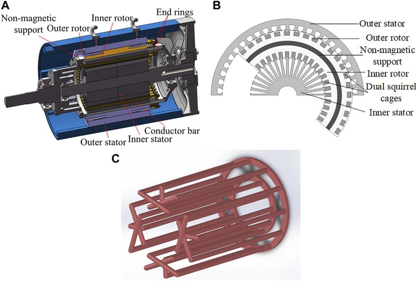
Zeng et al.                                                                                                                           Differential Cascading for DS-BDFIG

  FIGURE 3 | Interconnection between PR bars (4 pole pairs and 14 slots) and CR bars (2 pole pairs and 7 slots).

   Additionally, one more case also should be discussed                              TABLE 2 | Interconnection between PR and CR bars under PR with 4 pole pairs
                                                                                     and 14 slots, CR with 2 pole pairs and 7 slots.
                            pp  kpc      Zp  Zc                        (17)
                                                                                                                             CR                             PR
It can be known that Eq. 17 mismatches the condition of Eq. 13,
but a technique called the virtual slot method (VSM) is proposed                     Pole pair                                2                               4
                                                                                     Slot                                     7                              14
in this article to convert the SDCR into a joinable way. Hereto,
                                                                                     Electric phase angle                   102.8°                         102.8°
most possible slot/pole combinations have been covered by Eqs.                       Group I                       Bar No              α          Bar No               β
16, 17, and then the examples are introduced to establish the DS-                                                    1                 0             1                 0
BDFIM-SDCR based on the DC.                                                                                          2               102.8           2               102.8
                                                                                                                     3               205.6           3               205.6
                                                                                                                     4               308.4           4               308.4
pp = kpc and Zp = kZc                                                                                                5               411.2           5               411.2
When the pole pairs and the rotor slots of the power rotor (PR) are                                                  6                514            6                514
                                                                                                                     7               616.8           7               616.8
the k multiples of the control rotor (CR), the conductor bars of the                 Group II                        1                 0             8               719.6
PR and CR are cannot directly be connected due to their different                                                    2               102.8           9               822.4
slots. The solution is that k conductor bars in a slot in parallel                                                   3               205.6          10               925.2
connect to the k slots on the other side where one slot places one                                                   4               308.4          11               1,028
                                                                                                                     5               411.2          12              1,130.8
conductor bar. Generally, the rotor with the lower number of slots
                                                                                                                     6                514           13              1,233.6
has k conductor bars in one slot, while the rotor with the higher                                                    7               616.8          14              1,336.4
number of slots only arranges one conductor bar in one slot.
   An example of the PR with 4 pole pairs (14 slots) and the CR with
2 pole pairs (7 slots) is given in Figure 3, showing the
interconnection between PR and CR bars. Since the electrical                         of the same group are interconnected correspondingly in a positive-
phase angles α and β are calculated to be 102.8°, the PR and CR                      phase sequence way to building the DC.
are interconnected under the guidance of Eq. 12. Two conductor                           Figure 4 displays that the pole pairs of the PR and the CR are
bars should be settled in one slot of the CR, connecting two slots of                given by 3 and 2, while the slots of the PR and the CR are 12 and 8,
the PR. Table 2 tabulates the details of the interconnection between                 respectively. The PR and CR bars are interconnected according to
the PR and the CR. The conductor bars of the PR and the CR should                    Eq. 12 under k of improper fraction 3/2. Since the number of slots
be divided into two groups (k  2), namely groups I and II, to                       of the PR is not an integral multiple of the CR ones, the areas of
normalize the interconnection. Each group consists of 7 conductor                    the conductor bars for the PR and CR cannot be the same.
bars which occupy a 4π electric period owing to the electrical phase                 Therefore, a slot of the CR should be placed in two paralleled
angles α and β of 102.8°. On the basis of Eq. 12, the PR and CR bars                 conductor bars, one of which has 1 per-unit-area and the other is

Frontiers in Energy Research | www.frontiersin.org                               5                                          September 2021 | Volume 9 | Article 749424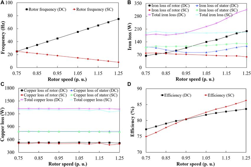
Zeng et al.                                                                                                                    Differential Cascading for DS-BDFIG

  FIGURE 4 | Interconnection between PR bars (3 pole pairs and 12 slots) and CR bars (2 pole pairs and 8 slots).

  FIGURE 5 | Interconnection between PR bars (2 pole pairs, 12 slots and 6 VSs) and CR bars (4 pole pairs and 12 slots).

0.5, and they are marked by the dashed and solid wires,                              cannot interconnect each other because of their different
respectively. Every slot of the PR is arranged one conductor                         electrical phase angles of the slots. A method of the virtual
bar with 1 per unit area except the slots of No. 5 to No. 8. The slots               slot (VS) is proposed to solve this problem, which enables the
of No. 5 to No. 8 all place two 0.5 per-unit-area conductor bars in                  PR and CR to obtain the same electrical phase angle.
parallel so that they are equivalent to the 1 per-unit-are in each                   The proposed method is illustrated as follows: k number of
slot, balancing with the other slots of the PR.                                      slots for the PR merge into one VS which occupies an electrical
                                                                                     phase angle so that the number of VSs for the PR is k multiples
pp = kpc and Zp = Zc                                                                 of the number of real slots of the CR, while the pole pairs of
If the pole pairs of the PR are k multiples of the CR and                            the PR and CR are invariant. In this way, the electrical
their rotor slots are identical, the calculated values of α and β                    angles for the real slots of the CR and the VSs of the PR
are unequal. The conductor bars of the PR and CR                                     are identical.

Frontiers in Energy Research | www.frontiersin.org                               6                                     September 2021 | Volume 9 | Article 749424
Zeng et al.                                                                                                                Differential Cascading for DS-BDFIG

TABLE 3 | Interconnection between PR and CR bars under PW with 2 pole pairs,
CW with 1 pole pairs and rotor slots of 40.

                                      CR                          PR

Pole pair                              1                           2
Slot                              40 (20 VSs)                     40
Electric phase angle               18°(VSs)                       18°
Group I                      Bar No             α        Bar No             β
                                1               0           1               0
                                3              18           2              18
                                5              36           3              36
                                7              54           4              54
                                9              72           5              72
                                «               «           «               «
                               33             288          17             288
                               35             306          18             306
                               37             324          19             324
                               39             342          20             342
Group II                        2               0          21             360
                                4              18          22             378
                                6              36          23             396
                                8              54          24             414
                               10              72          25             432
                                «               «           «               «
                               34             288          37             648
                               36             306          38             666
                               38             324          39             684
                               40             342          40             702

   Figure 5 shows the interconnection between the PR (2 pole
pairs and 12 slots) and the CR (4 pole pairs and 12 slots) bars.
Two real slots (k  1/2) are merged into one VS of the PR, taking
up the same electrical phase angle, and thus, connecting to two
conductor bars of the CR. The conductor bars are supposed to be
divided into four groups (pc  4) including group I (CR No. 1, 2, 3;
PR No. 1, 3, 5), group II (CR No. 4, 5, 6; PR No. 7, 9, 11), group III
(CR No. 7, 8, 9; PR No. 2, 4, 6), and group IV (CR No. 10, 11, 12;
PR No. 8, 10, 12), and hence, avoiding plenty of interconnections
of meaningless.

COMPARISON OF DS-BDFIM-SDCR WITH
DC AND SC
Interconnection of DS-BDFIM-SDCR
                                                                                     FIGURE 6 | Comparisons of rotor speed, active power, and voltage for
With DC                                                                              DC and SC modes (A) Rotor speeds versus CW frequency (B) CW and PW
A DS-BDFIM-SDCR with the PW of 2 pole pairs and the CW of 1                          active powers versus rotor speed (C) CW and PW voltages versus
pole pair based on the DC is modeled to validate the effectiveness                   rotor speed.
of doubly-fed operation and predict the electromagnetic
performance. The specification of the proposed machine is
tabulated in Table 1 where shows the numbers of slots for the
inner and outer rotors both of 40, conforming to the slot/pole                      CR are calculated to be 18° in terms of the PR with 2 pole pairs
combination of ppkpc and ZpZc. Since the electrical angles of                     and 40 real slots and the CR with 1 pole pair and 20 VSs. Two
the inner and outer rotors are not unequal, the VSM is utilized to                  groups should be divided (k  2) and meaningless connections of
solve the problem of interconnection. Two rotor slots of the inner                  different groups are forbidden. The odd and even NO. of CR bars
rotor are regarded as one VS so that two conductor bars of the CR                   are named by Groups I and II, respectively, and they both occupy
occupy the same electrical angle, connecting to the two slots of the                a 2π period. According to the interconnection rule of Eq. 12, the
outer rotor. The interconnection way of the PR and the CR is                        PR bars are arranged in sequence to connect the same electrical
given in Table 3. Both electrical phase angles of the PR and the                    phase angle of the CR bars.

Frontiers in Energy Research | www.frontiersin.org                              7                                  September 2021 | Volume 9 | Article 749424
Zeng et al. Differential Cascading for DS-BDFIG FIGURE 7 | Magnetic flux densities of DC and SC modes (A) DC mode (CW 12.5 Hz, PW 50 Hz, 3,750 r/min) (B) SC mode (CW 12.5 Hz, PW 50 Hz, 1,250 r/min). FIGURE 8 | Comparisons of rotor frequency, iron loss, copper loss and efficiency for DC and SC modes (A) Rotor frequencies versus rotor speed (B) Iron losses of rotor and stator versus rotor speed (C) Copper losses of rotor and stator versus rotor speed (D) Efficiencies versus rotor speed. Frontiers in Energy Research | www.frontiersin.org 8 September 2021 | Volume 9 | Article 749424
Zeng et al.                                                                                                              Differential Cascading for DS-BDFIG

TABLE 4 | Performance comparison between DC and SC modes under rated sub-natural and super-natural synchronous speeds.

                                                          Sub-natural synchronous speed                            Super-natural synchronous speed

Mode                                                       DC                           SC                           DC                              SC
Speed (r/min)                                            2,250                         750                         3,750                           1,250
Load (Ω)                                                   20                           20                           20                              20
PW voltage (V)                                           220.4                        220.6                         222                           220.85
PW current (A)                                            10.8                        10.74                        10.78                           10.53
CW voltage (V)                                            99.2                        114.8                         90.4                           120.3
CW current (A)                                            9.19                         9.19                         9.19                            9.19
PW frequency (Hz)                                          50                           50                           50                              50
CW frequency (Hz)                                        −12.5                        −12.5                         12.5                            12.5
Rotor frequency (Hz)                                       25                           25                           75                             8.33
Active power of PW (W)                                  −6,963                       −6,894                        −6,933                         −6,633
Reactive power of PW (Var)                                  0                            0                            0                               0
Power factor of PW                                          1                            1                            1                               1
Active power of CW (W)                                  1867.5                       2,449.5                       −1,365                        −2,390.1
Apparent power of CW (W)                                2,734.9                       3,165                       −2,492.3                       −3,316.67
Power factor of CW                                        0.68                         0.75                        0.548                            0.72
Flux linkage of PW (Wb)                                  0.746                         0.74                        0.746                           0.729
Flux linkage of CW (Wb)                                   0.91                         1.16                        0.997                            1.47
Current of conductor bar (A)                             232.6                        225.7                         230                             219
Current of outer and inner end rings (A)               723/1,443                    735/1,438                    721/1,442                       720/1,426
Resistance of PW (Ω)                                     1.32                          1.32                         1.32                            1.32
Resistance of CW (Ω)                                       1.3                          1.3                          1.3                             1.3
Resistance of rotor bar (Ω)                            1.678e-4                     1.678e-4                     1.678e-4                        1.678e-4
Resistance of inner end ring (Ω)                       1.467e-6                     1.467e-6                     1.467e-6                        1.467e-6
Resistance of outer end ring (Ω)                       2.227e-6                     2.227e-6                     2.227e-6                        2.227e-6
Copper loss of PW (W)                                    461.1                        457.2                        460.5                           439.5
Copper loss of CW (W)                                    329.5                        329.4                        330.3                           329.4
Copper loss of rotor (W)                                 558.2                        510.8                        518.7                           478.4
Total copper loss (W)                                   1,348.8                      1,297.4                      1,309.5                         1,247.3
Iron loss of inner stator (W)                             10.2                         11.6                          12                             17.1
Iron loss of outer stator (W)                             25.3                         26.5                         72.7                            24.9
Iron loss of inner rotor (W)                              39.4                         40.8                        126.4                            33.8
Iron loss of outer rotor (W)                              103                          97.9                        105.3                           113.1
Total copper loss (W)                                    177.9                        176.8                        316.4                           188.9
Efficiency (%)                                             76.9                         75.1                         83.6                            86.3

Performance Comparisons of                                                     rotor are 48, 36, and 40, respectively, and more information is
DS-BDFIM-SDCR With DC and SC                                                   listed in Table 1.
The merits of the DS-BDFIM-SDCR based on the DC are the                        Speed Range, Voltage and Power
wide speed range and the high natural synchronous speed to                     The speed ranges of the DC and SC modes are determined by the
obtain the comparable power density comparing to the SC mode,                  equivalent synchronous pole pairs. The variable speed range of the
while the drawback of the DC mode is the increment of the loss,                DC mode is much higher than that of the SC mode as shown in
decreasing the efficiency of the machine. The performance                       Figure 6A, displaying that the speed range of the DC mode starts
comparisons of the DC and the SC for the DS-BDFIM-SDCR                         from 2,250 to 3,750 r/min, whereas that of the SC mode works the
are discussed in this part to illustrate their characteristics. A DS-          doubly-fed operation from 750 to 1,250 r/min during the variation of
BDFIM-SDCR model with the PW of 2 pole pairs and the CW of                     the CW frequency from −12.5 to 12.5 Hz. Actually, the DS-BDFIM-
1 pole pair is adopted to predict the performance. The equivalent              SDCR with DC is a high-speed-low-torque machine and the SC
synchronous pole pairs based on the DC mode is 1 and those of                  mode appears the characteristic of low-speed-high-torque.
the SC mode is 3. The rated CW frequency is selected to be                         Benefiting from the high operating speeds, the DC mode acquires
±12.5 Hz so that the corresponding sub-natural synchronous and                 the electrical power comparable to the SC mode and this is validated
super-natural synchronous speeds of the DC mode are 2,250 and                  by Figure 6B which presents the absorbed or the output power of the
3,750 r/min, while those of the SC mode are given by 750 and                   PW and the CW. It is noted that the absorbed power of the winding is
1,250 r/min, respectively. The PW of the DS-BDFIM-SDCR,                        indicated by the positive value, while the minus values stand for the
whose rated phase voltage is 220 V, connects a load of 20 Ω,                   output power, and furthermore, the per-unit speed of the rotor is
outputting the rated electrical power of 7260 W. The CW is                     employed for graphing (3,000 r/min of the DC mode and 1,000 r/min
excited by the current source with the peak value of 13 A which                of the SC mode both expressed by 1 p. u.). The CW absorbs the active
keeps constant when the rotor speed changes. Besides, the                      power from the grid under the sub-natural synchronous speed and
numbers of slots for the inner stator, the outer stator and the                outputs the active power when the per-unit speed of the rotor is larger

Frontiers in Energy Research | www.frontiersin.org                         9                                  September 2021 | Volume 9 | Article 749424
Zeng et al. Differential Cascading for DS-BDFIG
TABLE 5 | Performance comparison between DS-BDFIM-SDCR and DS-BDFIM Figure 8A shows the rotor frequencies of the DC and SC
with wound rotor.
modes vary with the rotor speeds. As the rotor speed increases,
DS-BDFIM DS-BDFIM-SDCR the rotor frequency of the DC mode grows up, while that of the
with wound rotor SC mode declines. Evidently, at the super-natural synchronous
speed, the rotor frequency of the DC mode is much larger than
Mode Differential mode Differential mode
Speed (r/min) 3,750 3,750 the SC one, especially for the rated rotor speed of 1.25 p. u. The
Load (Ω) 20 20 expressions of the rotor frequency based on the DC mode at the
PW voltage (V) 220.5 222 sub-natural and super-natural synchronous speeds are
PW current (A) 10.85 10.78 respectively given by
PW frequency (Hz) 50 50
CW frequency (Hz) 12.5 12.5
⎪
⎧ f + fc
⎪
⎪ $$ p $$ pp − fp n > 1 p.u.
Rotor frequency (Hz) 75 75
⎪
⎪ $
$ pp − pc $$$
Active power of PW (W) −7,068 −6,933 ⎪
⎨ $
Reactive power of PW (Var) 0 0 fr ⎪ (18)
⎪
⎪ fp − fc
Power factor of PW 1 1 ⎪
⎪
Active power of CW (W) −1,245 −1,365 ⎩ $$$$
⎪ $$ pp − fp n < 1 p.u.
$
Resistance of PW (Ω) 1.3 1.32 $pp − pc $$
Resistance of CW (Ω) 1.51 1.3
Copper loss of PW (W) 459 460.5
The rotor frequency of the SC modes can be deduced by
Copper loss of CW (W) 342.6 330.3
⎪
⎧
⎪ fp + fc
Copper loss of rotor (W) 1,036.5 518.7 ⎪
⎪ fp − pp n > 1 p.u.
Total copper loss (W) 1838.1 1,309.5 ⎪
⎪ pp + pc
⎨
Iron loss of inner stator (W) 29.2 12 fr ⎪ (19)
Iron loss of outer stator (W) 112.8 72.7 ⎪
⎪ fp − fc
⎪
⎪
Iron loss of inner rotor (W) 112 126.4 ⎪
⎩ fp − p + p pp n < 1 p.u.
Iron loss of outer rotor (W) 172.9 105.3 p c
Total iron loss (W) 426.9 316.4
Efficiency (%) 78.6 83.6 Figure 8B compares the iron losses of the rotor and the stator as
well as the total losses for the DC and SC modes. The rotor iron
losses of the DC are much higher than those of the SC at different
speeds because the DC mode suffers from the high rotor
than 1, namely, the super-natural synchronous speed, both for the frequency except the low speed of 0.75 p. u. where the rotor
DC and the SC modes. As the rotor speed increases, the absolute CW frequencies of the DC and SC modes are the same. The iron loss is
power initially reduces and then rises because the CW frequency not only determined by the rotor frequency but also the magnetic
declines and then grows up, and simultaneously, the PW features the flux density so that the iron losses of the SC stator are higher than
constant active power outputs. The absolute CW power of the DC is those of the DC stator at full range speeds due to the higher
always lower than that of the SC in a variety of speeds, implying that magnetic flux density of the SC stator as shown in Figure 7. As a
the total active power outputs of the DC at sub-natural synchronous result of a mix of the rotor frequency and the magnetic flux
speeds are higher than that of the SC, while they are evidently low density, the total losses of the DC mode are greatly higher than
under super-natural synchronous speeds comparing to the SC mode. the SC one at the super-natural synchronous speeds, while they
Figure 6C reveals the variation of the CW and PW voltages at are below the SC mode at the sub-natural synchronous speeds.
various rotor speeds for the DC and SC modes. The phase The copper losses of the rotor and stator versus the rotor speed
voltages of the PW stay 220 V both for the DC and SC though for the DC and SC modes are compared in Figure 8C, showing
there is a little fluctuation for the DC mode. The CW voltages of that the copper losses of the DC and SC stators are almost the
the DC and the SC gradually decrease and then increase, along same, whereas those of the SC rotor are lower than the those of
with the increment of the rotor speed. The nearer to the natural- the DC rotor due to the higher rotor frequency for the DC.
synchronous speed, the lower CW voltage needs and the lower However, their difference seems to be small because the
CW power factor appears. The CW voltage of the SC is higher maximum rotor frequency of the DC mode is only 75 Hz
than the DC one at the full speed range owing to the fact that the which lays a small impact on the copper loss. Therefore, the
absolute power of the CW for the SC mode is higher than that of total copper loss of the DC shows a little bit bigger than that of
the DC mode as shown in Figure 6B. Also, the magnetic flux the SC.
density of Figure 7 shows that the inner stator and rotor of the SC Figure 8D exhibits the efficiencies at various rotor speeds
mode have a higher value than those of the DC mode, and thus, under the DC and SC modes. The efficiencies of the DC mode are
more CW voltages for excitation. superior to those of the SC mode at the sub-natural synchronous
speeds, while at the super-natural synchronous speeds they are
Rotor Frequency, Iron Loss, Copper Loss and worse. The significant reason for the DC mode with higher
Efficiency efficiency at the sub-natural synchronous speeds comparing to
The other aspect that should be discussed between the DC and SC the SC mode is that the DC mode offers lower CW voltage, thus
modes is their difference in the rotor frequency and what reducing the absorbed power and increasing the total power
consequences it causes. outputs. At the super-natural synchronous speeds, the DC mode
Frontiers in Energy Research | www.frontiersin.org 10 September 2021 | Volume 9 | Article 749424Zeng et al. Differential Cascading for DS-BDFIG
FIGURE 9 | Prototype of DS-BDFIM-SDCR with sum mode.
has higher rotor frequencies than the SC mode, and thus higher mode with the rotor frequency of 75 Hz (at 3,750 r/min) brings
rotor iron losses, higher copper losses as well as lower efficiencies. about the iron loss of 316.4 W, while the SC mode with the rotor
Table 4 tabulates the detailed performance comparison frequency of 8.33 Hz (at 1,250 r/min) leads to the iron loss of
between the DC and SC modes under rated sub-natural and 188.9 W, contributing the higher efficiency of the SC mode
super-natural synchronous speeds. The efficiency calculation of (86.3%) than the DC mode (83.6%). To sum up, it can be
the DS-BDFIM-SDCR is given by concluded that the DC mode behaves better than the SC mode
Pp + Pc at sub-natural synchronous speed, but its iron and copper losses
η (20) at super-natural synchronous speed are supposed to be further
Pp + Pc + Piron + Pcopper
optimized.
where Pp and Pc are the outputted or absorbed powers, while Piron To validate the superiority of the DS-BDFIM-SDCR with the
and Pcopper are the total copper loss and total iron loss of the differential mode, the performance comparison between the DS-
machine, respectively. BDFIM-SDCR and the DS-BDFIM with wound rotor in (Han
When the DC mode with 2,250 r/min and the SC mode with et al., 2017) is shown in Table 5. The copper loss of the PW and
750 r/min, their rotor frequencies are the same, resulting in the CW between the two machines are similar, however, the copper
same total iron losses (177.9 and 176.8 W, respectively) loss of the rotor for the DS-BDFIM with wound rotor is almost
approximately. Since the absorbed active power of the CW twice of the DS-BDFIM-SDCR ones, verifying the advantages of
based on the DC mode (1867.5 W) is significantly lower than the low resistance of squirrel cage rotor comparing to the wound
that of the SC one (2,449.5 W), the DC mode (76.9%) performs rotor. Furthermore, the total iron loss of the DS-BDFIM with
more efficiently comparing to the SC mode (75.1%). The DC wound rotor is also higher than that of the DS-BDFIM-SDCR.
Frontiers in Energy Research | www.frontiersin.org 11 September 2021 | Volume 9 | Article 749424Zeng et al. Differential Cascading for DS-BDFIG
FIGURE 10 | Experimental measurement of CW voltages, CW currents, PW voltages, PW currents, efficiencies from 750 r/min to 1,250 r/min (A) 750 r/min (CW
-12.5 Hz, PW 50 Hz and 20 ms/div) (B) 1,250 r/min (CW 12.5Hz, PW 50 Hz and 50 ms/div) (C) 750 r/min to 1,250 r/min (D) Efficiencies versus rotor speeds.
Therefore, the DS-BDFIM-SDCR based on the differential modes min, respectively. The waveforms of the PW voltages and
with the efficiency of 83.6% is obviously higher than the efficiency currents exhibit sinusoidal distributions, verifying the low
of 78.6% for the DS-BDFIM with wound rotor. harmonics of the DS-BDFIM-SDCR.
The voltages and currents of both PW and CW versus the
rotor speeds from 750 to 1,250 r/min are measured in
EXPERIMENT Figure 10C. The PW line voltages at different speeds stay the
same of 380 V. The CW voltage declines initially and then grows
The DS-BDFIM-SDCR with sum mode is prototyped as shown in up. As the speed increases, the CW current exhibits a small
Figure 9. The core component of the prototype is the SDCR, one change except for the natural-synchronous speed of 1,000 r/min
end of which is short-circuited by two copper rings, while the where the direct source is excited, while the PW current
other end is formed by the staggered connection. Since the copper maintains the same due to the constant resistance load. The
bars are hard to achieve the staggered interconnection in the end experimental measurement of efficiency versus rotor speeds from
when the prototype is manufacturing, they are replaced by soft 750 to 1,250 r/min is given in Figure 10D, showing the
parallel enameled wires so as to facilitate implementation. efficiencies increases along with the rotor speeds except for the
The CW with the excitation of the voltage source and the PW natural speed of 1,000 r/min.
with a load of 100 Ω to enable the prototype of the doubly-fed
operation. Figures 10A,B shows the measured PW voltages
(50 Hz), CW voltages (±12.5 Hz), PW currents and CW CONCLUSION
currents at 750 and 1,250 r/min. To obtain the rated PW line
voltage of 380 V, the CW is excited with the root mean square In this article, the design method of the DC for the DS-BDFIM-
(RMS) line voltages of 166 V at 750 r/min, and 205.6 V at 1,250 r/ SDCR is proposed to solve the issues of high rotor leakage and
Frontiers in Energy Research | www.frontiersin.org 12 September 2021 | Volume 9 | Article 749424Zeng et al. Differential Cascading for DS-BDFIG
low capacity of magnetic field conversion of the conventional DATA AVAILABILITY STATEMENT
differential-mode-based BDFM. The proposed method enables
the high number of conductor bars for the cage rotor even with The original contributions presented in the study are included in
the low synchronous pole pairs of |p1-p2|, achieving reduced rotor the article/supplementary material, further inquiries can be
flux leakage. The rotating MMF theory is utilized to deduce the directed to the corresponding author.
conditions that should be satisfied for the SDCR. Based on the
result of derivation, two situations of pole/slot combinations are
taken into account and examples are illustrated to introduce the AUTHOR CONTRIBUTIONS
details of interconnection of the SDCR. The FE models of the DS-
BDFIM-SDCR with DC and SC are built to compare their YZ did the conceptual design, simulation analysis and writing of the paper.
electromagnetic performance. The results show that the DC MC revised and improved the article. XY and CZ organized case studies.
mode of the DS-BDFIM-SDCR exhibits better performance
than the SC one at the sub-synchronous-speed region such as
lower CW excitation, lower iron loss and higher efficiency, while FUNDING
at the super synchronous-speed region, the DC mode suffers from
higher copper loss and iron loss due to the increased rotor This work was supported in part by the National Natural Science
frequency comparing to the SC mode, and hence, lower Foundation of China (NSFC) under Grant 61973073 and the
efficiency. Therefore, the iron and copper losses are ought to Scientific Research Foundation of Graduate School of Southeast
be further optimized. University under Project YBPY 1878.
Journal of Power and Energy Systems (IEEE), 1–18. doi:10.17775/
REFERENCES CSEEJPES.2020.03590
Yin, J. (2021). Research on Short-Circuit Current Calculation Method of Doubly-
Cheng, M., and Zhu, Y. (2014). The State of the Art of Wind Energy Conversion Fed Wind Turbines Considering Rotor Dynamic Process. Front. Energ. Res. 9,
Systems and Technologies: a Review. Energ. Convers. Manag. 88, 332–347. 1–7. doi:10.3389/fenrg.2021.686146
doi:10.1016/j.enconman.2014.08.037 Zeng, Y., Cheng, M., Wei, X., and Xu, L. (2020). Dynamic Modeling and
Cheng, Y., Yu, B., Kan, C., and Wang, X. (2020). Design and Performance Study of Performance Analysis with Iron Saturation for Dual-Stator Brushless
a Brushless Doubly Fed Generator Based on Differential Modulation. IEEE Doubly Fed Induction Generator. IEEE Trans. Energ. Convers. 35, 260–270.
Trans. Ind. Electron. 67, 10024–10034. doi:10.1109/TIE.2019.2962430 doi:10.1109/TEC.2019.2942379
Han, P., Cheng, M., Ademi, S., and Jovanovic, M. G. (2018). Brushless Doubly-Fed Zeng, Y., Cheng, M., Wei, X., and Zhang, G. (2021). Grid-connected and
Machines: Opportunities and Challenges. Chin. J. Electr. Eng. 4, 1–17. Standalone Control for Dual-Stator Brushless Doubly Fed Induction
doi:10.23919/cjee.2018.8409345 Generator. IEEE Trans. Ind. Electron. 68, 9196–9206. doi:10.1109/
Han, P., Cheng, M., Jiang, Y., and Chen, Z. (2017). Torque/power Density TIE.2020.3028824
Optimization of a Dual-Stator Brushless Doubly-Fed Induction Generator Zhang, F., Yu, S., Wang, Y., Jin, S., and Jovanovic, M. G. (2019). Design and
for Wind Power Application. IEEE Trans. Ind. Electron. 64, 9864–9875. Performance Comparisons of Brushless Doubly Fed Generators with Different
doi:10.1109/TIE.2017.2726964 Rotor Structures. IEEE Trans. Ind. Electron. 66, 631–640. doi:10.1109/
Li, H., Liu, H., and Xu, B. (2019). “A New Experimental Method of Brushless TIE.2018.2811379
Doubly-Fed Machine Based on Differential Mode,” in 2019 IEEE 8th Joint Zhang, K., Zhou, B., Or, S. W., Li, C., Chung, C. Y., and Voropai, N. I. (2021).
International Information Technology and Artificial Intelligence Conference “Optimal Coordinated Control of Multi-Renewable-To-Hydrogen Production
(ITAIC) (IEEE), 1159–1163. doi:10.1109/itaic.2019.8785732 System for Hydrogen Fueling Stations,” in IEEE Transactions on Industry
Okedu, K. E., Ai Tobi, M., and Ai Araimi, S. (2021). Comparative Study of the Applications (Early Access) (IEEE), 1. doi:10.1109/TIA.2021.3093841
Effects of Machine Parameters on DFIG and PMSG Variable Speed Wind
Turbines during Grid Fault. Front. Energ. Res. 9, 1–13. doi:10.3389/ Conflict of Interest: The authors declare that the research was conducted in the
fenrg.2021.655051 absence of any commercial or financial relationships that could be construed as a
Pan, W., Chen, X., and Wang, X. (2021). Generalized Design Method of the Three- potential conflict of interest.
phase Y-Connected Wound Rotor for Both Additive Modulation and
Differential Modulation Brushless Doubly Fed Machines. IEEE Trans. Energ. The reviewer QW declared a shared affiliation with the authors YZ, MC, XY, CZ to
Convers. 36, 1940–1952. doi:10.1109/TEC.2020.3045061 the handling editor at the time of the review.
Roberts, P. C. (2004). A Study of Brushless Doubly-Fed (Induction) Machines.
Cambridge: University of Cambridge. Publisher’s Note: All claims expressed in this article are solely those of the authors
Ruviaro, M., Runcos, F., Sadowski, N., and Borges, I. M. (2012). Analysis and Test and do not necessarily represent those of their affiliated organizations, or those of
Results of a Brushless Doubly Fed Induction Machine with Rotary Transformer. the publisher, the editors and the reviewers. Any product that may be evaluated in
IEEE Trans. Ind. Electron. 59, 2670–2677. doi:10.1109/TIE.2011.2165457 this article, or claim that may be made by its manufacturer, is not guaranteed or
Shiyi Shao, S., Abdi, E., and McMahon, R. (2012). Low-cost Variable Speed Drive endorsed by the publisher.
Based on a Brushless Doubly-Fed Motor and a Fractional Unidirectional
Converter. IEEE Trans. Ind. Electron. 59, 317–325. doi:10.1109/ Copyright © 2021 Zeng, Cheng, Yan and Zhang. This is an open-access article
TIE.2011.2138672 distributed under the terms of the Creative Commons Attribution License (CC BY).
Williamson, S., Ferreira, A. C., and Wallace, A. K. (1997). Generalised Theory of The use, distribution or reproduction in other forums is permitted, provided the
the Brushless Doubly-Fed Machine. Part 1: Analysis. IEE Proc. Electr. Power original author(s) and the copyright owner(s) are credited and that the original
Appl. 144, 111–122. doi:10.1049/ip-epa:19971051 publication in this journal is cited, in accordance with accepted academic practice.
Xiong, L., Liu, X., Liu, Y., and Zhuo, F. (2020). “Modeling and Stability Issues of No use, distribution or reproduction is permitted which does not comply with
Voltage-Source Converter Dominated Power Systems: a Review,” in CSEE these terms.
Frontiers in Energy Research | www.frontiersin.org 13 September 2021 | Volume 9 | Article 749424You can also read